Supplement of Response of dust emissions in southwestern North America to 21st century trends in climate, CO2 fertilization, and land use: ...
←
→
Page content transcription
If your browser does not render page correctly, please read the page content below
Supplement of Atmos. Chem. Phys., 21, 57–68, 2021
https://doi.org/10.5194/acp-21-57-2021-supplement
© Author(s) 2021. This work is distributed under
the Creative Commons Attribution 4.0 License.

Supplement of
Response of dust emissions in southwestern North America to
21st century trends in climate, CO2 fertilization, and land use:
implications for air quality
Yang Li et al.

Correspondence to: Yang Li (yangli@seas.harvard.edu)

The copyright of individual parts of the supplement might differ from the CC BY 4.0 License.
13

14   Figure S1. Changes in land use fraction in southwestern North America from 1990 to 2015. Future

15   land use scenarios applied follow CMIP5. Land use types of cropland, pasture, and urban area are

16   plotted on the left, and the sum of these three types is plotted on the right.

17

                                                                                                   2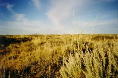
18

               ΔMean Temperature                        ΔPrecipitation

                                                                                     kg m-2 mon-1
19

20   Figure S2. GISS-E2-R simulated spring averaged monthly mean temperature and precipitation

21   in southwestern North America for RCP8.5. Changes are between the present day and 2100, with

22   five years representing each time period. The color bar is reversed for precipitation, with redder

23   colors indicated drier conditions.

24

25   Evaluation of dust emissions based on LPJ-LMfire

26          Figure S3 shows the simulated present-day (2011-2015) distribution of vegetation area

27   index (VAI) over southwestern North America. Values are derived from LAI generated by the

28   LPJ-LMfire dynamic vegetation model, as described in the main text. We find relatively high VAI

29   values in central Arizona, northern New Mexico, northern Texas, and northwestern Mexico, but

30   near-zero VAI in the arid regions of western Texas and along the northern Mexico border. Figure

31   S4 compares the differences in springtime VAI generated by LPJ-LMfire for the present day and

32   that derived from 1-km reflectance data from the Advanced Very High Resolution Radiometer

33   (AVHRR, Bonan et al., 2002). This satellite-based VAI is the default dataset in the DEAD module

34   (Zender et al., 2003). The differences between these two VAI datasets are mostly small, within ±1

                                                                                                          3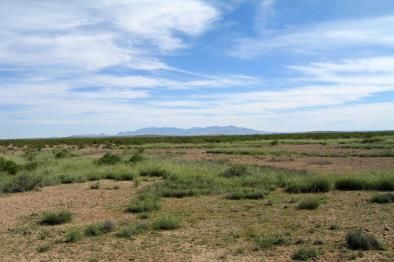
35 m2 m-2, across southwestern North America, giving us confidence in the performance of LPJ-
36 LMfire. In addition, we categorize the LPJ-LMfire simulated land cover types as trees and shrubs,
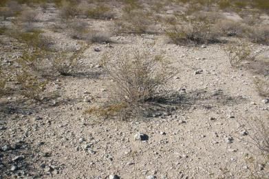
37 grasses, and barren land (Figure S5). The high-dust emission region shown in Figure S3 is
38 dominated by grass ecosystems and barren land, roughly consistent with observed land cover
39 shown in the photos of four locations (southwest New Mexico, southeast New Mexico, west Texas,
40 and northern Chihuahua state, Mexico) selected from the principle dust-producing regions in our
41 study (Figure S5).
42 The dominant plant functional types in LPJ-LMfire in the southwestern North America
43 include temperate needleleaf evergreen, temperate broadleaf evergreen, temperate broadleaf
44 summergreen, and C3 perennial grass, roughly consistent with observed, present-day vegetation
45 types (McClaran and Van Devender, 1997). We acknowledge, however, that with only nine PFTs,
46 LPJ-LMfire cannot capture the phenology of all plant species, which could in turn introduce error
47 into our dust calculations. Still, the relatively good match of modeled springtime VAI with that
48 observed is encouraging.
49 Figure S3 also shows the distribution of dust emissions for the present-day RCP4.5
50 scenario, with especially high emissions simulated over those areas with near zero VAI. We apply
51 these emissions to GEOS-Chem and evaluate the resulting fine dust concentrations using ground-
52 based measurements from the Interagency Monitoring of Protected Visual Environments
53 (IMPROVE) network (Malm et al., 2004). Hand et al., 2016 used the observed iron content from
54 IMPROVE as a proxy for fine dust concentrations, and approximated soil-derived PM2.5 as PM2.5-
55 Iron/0.058. IMPROVE dust observations are made every three days, and we show the spatial or
56 temporal median of these observations as outliers are common in the dataset, and GEOS-Chem is
57 unlikely to capture the extreme dust events. For model validation, we rely on the RCP8.5 results
4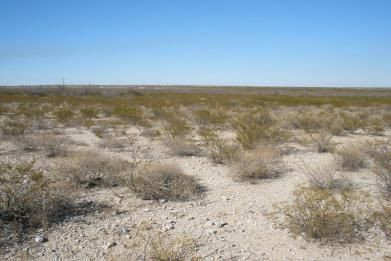
58 for 2011-2015, which yields nearly identical results as RCP4.5. GEOS-Chem tracks fine dust with
59 a diameter range of 0.2-2.0 μm, while the IMPROVE approximation yields dust concentrations
60 with diameter less than 2.5 g m-3. This disparity may hinder the model comparison with
61 observations.
62 Figure S6 compares the spatial distribution of GEOS-Chem springtime dust concentrations
63 with observations, and Figure S7 examines the temporal variability of modeled and observed dust
64 averaged over the region. In general, the model captures both the observed spatial and temporal
65 variability, though GEOS-Chem underestimates dust at a few sites in Arizona. This underestimate
66 could be a result of abundant mountain vegetation simulated by LPJ that alleviates dust generation
67 from persistently arid or desert regions. The 2011-2015 timeseries of observed and modeled dust
68 (Figure S7) reveals that GEOS-Chem exhibits a smaller seasonal variation of 0.2-3.1 μg m-3,
69 compared with the observed range of 0.2-8.1 μg m-3. Overall, we find that the present-day
70 simulations reasonably reproduce observed fine dust over southwestern North America.
5
71

72   Figure S3. Present-day (2011-2015) spring averaged VAI and fine dust emissions for the RCP8.5

73   fixed-CO2 case in southwestern North America, in which CO2 fertilization is neglected. VAI

74   results are from LPJ-LMfire. Dust emissions are generated offline using the GEOS-Chem emission

75   component (HEMCO).

76

77

78   Figure S4. Differences between springtime VAI simulated by LPJ-LMfire and that derived from

79   1-km satellite data in southwestern North America. The LPJ-LMfire results are the mean 2011-

80   2015 values from the RCP8.5 fixed-CO2 case; satellite-derived VAI are from Bonan et al. (2002).

                                                                                                  6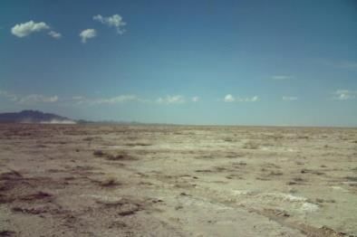
81

82

     103.25°W 31.25°N (West Texas)
     LPJ: 0.3% trees/shrubs, 74.9% grass, 24.8% unvegetated

     The Degree Confluence Project, 2011    Google Street View, 2013   The Degree Confluence Project, 2011

     104.25°W 33.25°N (Southeast New Mexico)
     LPJ: 0.5% trees/shrubs, 73.4% grasses, 20.1% unvegetated

      The Degree Confluence Project, 1999   Google Street View, 2013   Google Street View, 2013
83

                                                                                                             7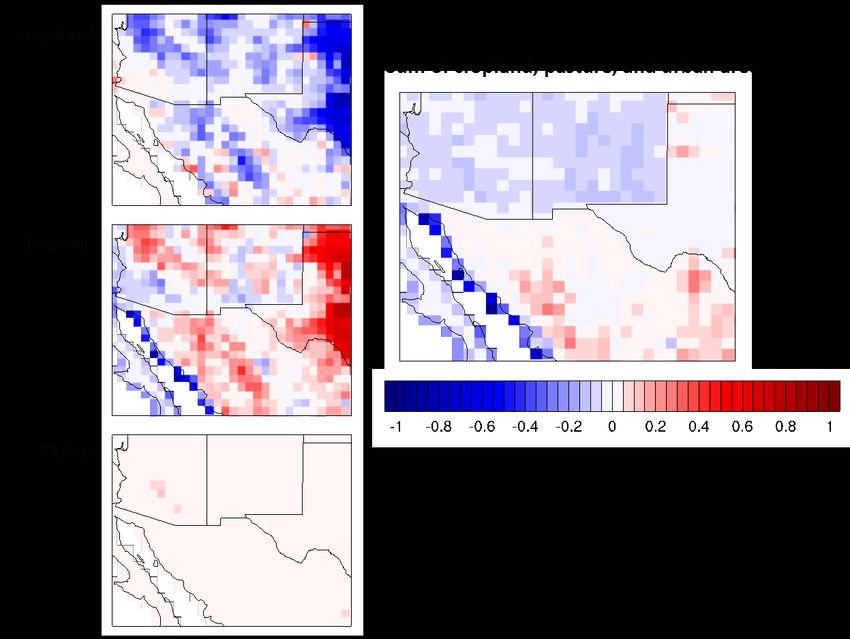
108.25°W 32.25°N (Southwest New Mexico)
      LPJ: 12.7% trees/shrubs, 73.3% grasses, 14.0% bare ground

        Google Street View, 2014              The Degree Confluence Project, 2014   The Degree Confluence Project, 2014

      107.25°W 31.25°N (Chihuahua state, Mexico)
      LPJ: 2.4% trees/shrubs, 65.3% grasses, 32.2% bare ground

        The Degree Confluence Project, 2005   Google Street View, 2019              Google Street View, 2018
84

85   Figure S5. Top panels show mean fractional land cover of trees, grasses, and barren land averaged

86   over 2006-2015, as simulated by LPJ-LMfire. Purple stars on the top lefthand panel mark four

87   selected locations that are broadly representative of vegetation within the principle dust-producing

88   regions in our study, with photographs of each location shown below. Latitude and longitude

89   values listed above each row of photographs denote the center of the LPJ-LMfire gridcell, and the

90   corresponding photographs are all taken within the area encompassed by the 0.5° × 0.5° gridcell.

91   Credits for photographs from the Degree Confluence Project (www.confluence.org) are as follows:

92   Alan B. (west Texas), Matt Taylor and Scott Kessel (southeast New Mexico), Jerry Heikkinen and

93   Shawn Fleming (southwest New Mexico), and Luis Baca (Chihuahua, Mexico).

94

                                                                                                                          8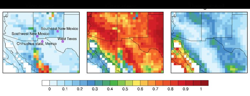
95

 96

 97   Figure S6. Spring fine dust concentration. Circles represent ground-based observations from the

 98   IMPROVE network, shown as the medians at each site over 2011-2015. The colored background

 99   is from GEOS-Chem simulations with the present-day (2011-2015) fine dust emissions for the

100   RCP8.5 fixed-CO2 case at 0.5° x 0.625° spatial resolution.

101

                                                                                                   9
102
103
104 Figure S7. Seasonal cycle of GEOS-Chem simulated and IMPROVE observed fine dust
105 concentrations, shown as the medians over southwestern North America from 2011 to 2015. The
106 red dots represent the median of IMPROVE observations taken over all sites in the region at each
107 measurement timestep. IMPROVE has a measurement frequency of every three days. The solid
108 line shows GEOS-Chem simulated variations at 0.5° x 0.625° resolution for the 2010 time slice
109 for the RCP8.5 fixed-CO2 case.
10110
111
112 Figure S8. Contributions of CO2 fertilization and anthropogenic land use to changes in VAI in
113 spring in southwestern North America for RCP4.5 and RCP8.5. Changes are between the present
114 day and 2100, with five years representing each time period. The top row is for CO 2 fertilization,
115 and the bottom row is for land use trends. Results are from LPJ-LMfire.
116
11117
118 Figure S9. Changes in yearly averaged land use fraction in southwestern North America for
119 RCP4.5 and RCP8.5 between the present day and 2100, with five years representing each time
120 period. Future land use scenarios applied follow CMIP5. Land use plotted here is the sum of
121 cropland, pasture, and urban area.
122
12123
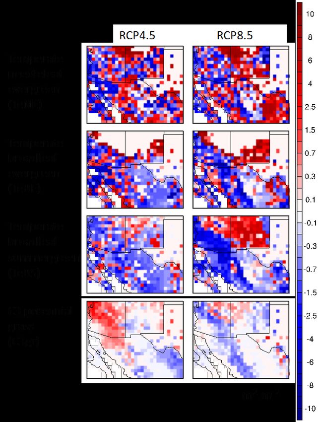
124 Figure S10. Simulated changes in springtime averaged LAI for the four dominant plant functional
125 types (PFTs) in southwestern North America under RCP4.5 and RCP8.5 for the fixed-CO2
126 condition, in which CO2 fertilization is neglected. Changes are between the present day and 2100,
127 with five years representing each time period. For clarity, the increments in the color bar are
128 unevenly distributed. Results are from LPJ-LMfire.
129
130
131
132
13133 References
134 Bonan, G. B., Levis, S., Kergoat, L., and Oleson, K. W.: Landscapes as patches of plant functional
135 types: An integrating concept for climate and ecosystem models, Global Biogeochemical Cycles,
136 16, 5-1-5-23, 2002.
137 Hand, J., White, W., Gebhart, K., Hyslop, N., Gill, T., and Schichtel, B.: Earlier onset of the spring
138 fine dust season in the southwestern United States, Geophysical Research Letters, 43, 4001-4009,
139 2016.
140 Malm, W. C., Schichtel, B. A., Pitchford, M. L., Ashbaugh, L. L., and Eldred, R. A.: Spatial and
141 monthly trends in speciated fine particle concentration in the United States, Journal of
142 Geophysical Research: Atmospheres, 109, 2004.
143 McClaran, M. P., and Van Devender, T. R.: The desert grassland, University of Arizona Press,
144 1997.
145 Zender, C. S., Bian, H., and Newman, D.: Mineral Dust Entrainment and Deposition (DEAD)
146 model: Description and 1990s dust climatology, Journal of Geophysical Research: Atmospheres,
147 108, 2003.
148
14You can also read