TECHNICAL MEMO ON CITYWIDE HEAT MODELING - APPENDIX

APPENDIX 1

TECHNICAL MEMO ON
CITYWIDE HEAT MODELING

Boston Heat Resilience Study
Technical overview of the urban heat island
modelling methodology.

May 12, 2021

For
The City of Boston and Sasaki Associates

By
Klimaat Consulting & Innovation Inc.
Meiring Beyers, PhD, Director
meiring.beyers@klimaat.ca

 1

Summary of Datasets Issued from the Citywide Heat Modeling

The datasets issued and used in the Heat Resilience Strategies for City of Boston is
based on a weeklong hourly analysis period for the week of July 18-24, 2019. This period
was chosen in collaboration with the City of Boston to model a period that coincided
with a reported strong heat wave event in the recent past.

 • Air Temperature (Ta): This dataset shows the spatial distribution of the near
 surface modelled air temperature (°F) during the afternoon (3pm) or night (3am)
 of the warmest day of the analysis week. This dataset helps to identify the
 relatively warmer (or cooler) areas during a hot day, and areas that retain (or
 shed) heat during the night.

 • Heat Event Duration (HED): The heat event duration is the duration (hours) that
 modelled heat conditions may exceed a heat alert level for the analysis week. The
 Boston heat advisory protocol determines whether to issue a heat advisory, alert,
 or emergency based on forecasted weather conditions exceeding certain heat
 index thresholds. The HED dataset issued shows the modelled number of hours
 during the analysis week that the heat index, as defined by the National Weather
 Service, may exceed a threshold temperature of 95°F for days when the daytime
 low temperature does not drop below 75°F (heat alert level). The HED dataset is
 useful to highlight which neighbourhood areas may stay above a heat alert level
 for the longest period during a hot week.

 • Urban Heat Island Intensity (UHII): The UHII is a measure of the daily intensity
 and duration of the urban heat condition relative to the regional (rural) condition.
 The UHII dataset uses the entire weeklong hourly analysis dataset and sums the
 hourly difference between the local and rural air temperature before averaging
 this by day i.e.,
 
 24
 = ∑( − )
 
 1

 The issued UHII index divides the UHII by 24 hours to show the UHII as an
 average daily temperature difference (°F) above the rural temperature. The UHII
 dataset helps to highlight areas that remain hot and for longer and is therefore
 reflective of both the intensity and the duration of localised heat within the city
 during a hot week.

Contents
 1. Introduction ...................................................................................................................................................................... 3
 2. Urban Heat Islands ......................................................................................................................................................... 3
 2.1 Surface urban heat island (SUHI) analysis ..................................................................................................... 4
 2.2 Canopy urban heat island (UHI) modelling methodology...................................................................... 5
 3. Urban Heat Modelling Runs .................................................................................................................................... 12
 3.2 Case Study: July 10-17, 2016............................................................................................................................ 12
 3.3 Case Study: July 18-25, 2019............................................................................................................................ 14
 4. Summary ......................................................................................................................................................................... 16
References ................................................................................................................................................................................ 17

 2

1. Introduction
This report is part of the work covered in the Boston Heat Resilience study initiated by the City of
Boston and led by Sasaki Associates. The report aims to provide a high-level overview of the
technical methodology used by Klimaat Consulting & Innovation Inc. (“Klimaat”) to model the
urban heat island characteristics across the Boston Municipality (“Boston”). The modelling work is
performed to help the design team and the city stakeholders visualise and evaluate the spatial and
temporal distribution of urban heat across the city. This report does not intend to be a complete
scientific description of the urban Land Use and Land Cover (LULC) influences on urban climatic
characteristics and focusses mainly on the overview of the heat modelling and mapping
methodology as applied to the heat resilience study.

The specific purpose of the work performed here was to generate georeferenced data (map) layers
that allow for a spatial and temporal evaluation of the distribution of urban heat island
characteristics within and around Boston. It aims to compliment and support the work performed
earlier by others as part of the Climate Ready Boston initiatives.

2. Urban Heat Islands
Urban heat island effects are typically evaluated or defined as the difference between localised
urban climatic conditions and the conditions further away from the urban centres such as within its
suburbs and the rural outskirts. Many textbooks are available that describe these urban climatic
processes in detail, such as Oke et al (Oke, 2017). In general, a combination of urban land use and
land cover (LULC) characteristic may modify the surface and near surface energy exchanges with the
urban atmosphere that causes climatic differences between rural and urban landscapes. These
influences include, but are not limited to,

 • increased hardscape and or limited or different urban vegetation cover that alters the
 amount of solar radiation intercepted by the urban fabric and modifies the latent heat
 contribution to the near surface energy exchange,

 • increased urban massing that changes the ventilating wind flow characteristics within urban
 streets and neighbourhoods and affects the sensible heat contributions within the urban
 setting,

 • increased urban massing and its form alters the shading and sky view factors especially
 within denser city contexts which affects the shortwave and longwave radiation exchange
 within the city,

 • differences in urban land cover thermal specifications, such as reflectance, emissivity, heat
 capacity, material density and moisture content, that changes the local heat transfer and
 thermal storage characteristics within the urban fabric, and

 3

• athropogenic heat sources i.e., the additional energy (heat) released into the urban setting
 due to human activities such as from heating or cooling of buildings, and from operating
 transport vehicles, to name a few sources.

When studying urban heat island effects, it is important to distinguish between, at least, surface and
canopy heat island characteristics:

 • surface urban heat island (SUHI) effects are urban-rural differences of surface temperatures,
 and

 • canopy urban heat island (UHI) effects are urban-rural differences of air temperature in the
 near surface urban canopy layer i.e., roughly the layer between the surface and the urban
 massing height.

This distinction is important. High surface temperatures are often recorded during daytime within
urban settings, such as solar exposed areas with low reflectance (albedo). These areas may include
dark roof tops, asphalt covered parking lots, or even exposed natural or artificial grass surfaces or
bare soil and are often also associated with higher local air temperatures. However, these enhanced
daytime surface and air temperature characteristics may exhibit different characteristics at night, as
the same exposure can also help it to cool more rapidly and generate cooler air temperatures. Thus,
a high daytime surface and air temperature difference (high SUHI & UHI) may often diminish at
night. Similarly, areas with dense urban massing may have comparably cooler daytime surface and
near-surface air temperatures due to reduced grade level interception of solar radiation and
enhanced thermal energy storage in the urban fabric. However, at night the denser urban form may
be more effective in trapping the stored thermal energy by limiting re-radiation and sensible heat
transfer and thereby heating the near surface atmosphere creating warmer air temperatures at
night compared to rural surroundings.

As such there is benefit to evaluate urban heat island characteristics in terms of surface temperature
(SUHI) and canopy air temperature (UHI) to identify areas that are hot during daytime, hot during
nighttime, or potentially worse for summer heat wave conditions, hot during day and nighttime i.e.,
prolonged diurnal heat wave conditions. This forms the main purpose of the work; to contribute to
the study of the urban heat characteristics in Boston to provide spatial and temporal SUHI and UHI
data. In the following section a high-level overview is provided of the urban heat modelling and
analysis methodology applied in this work.

2.1 Surface urban heat island (SUHI) analysis
Surface heat island effects are often studied by means of remotely sensed data to generate Land
Surface Temperatures (LST) maps from multispectral satellite data such as Landsat 8
(https://landsat.gsfc.nasa.gov/landsat-8/landsat-8-overview). The purpose here was not to generate
new LST maps for Boston from Landsat multispectral satellite data, as this effort is thoroughly
covered in work performed by other groups. Instead, it aims to compliment the existing Boston
heat map datasets, as currently used by the city for understanding its spatial heat distribution

 4

characteristics, with additional urban canopy heat island (UHI) information. However, Landsat 8
derived LST datasets were produced in this work but were mainly used to test the performance of
the urban canopy urban heat island modelling process (K-UCMv1), described below, as hourly
surface temperature data is also one of the resolved and exported variables. This makes it useful for
independent comparison between the LST information obtained from Landsat and that derived
from the urban canopy modelling.

In the current work a LST map was generated based on a Landsat 8 image data taken on July 13,
2016. The land surface data is derived based on the 30m resolution multispectral bands and the
100m resolution thermal bands. The processing is based on a well-established radiative transfer
model approach, as described by Peng et al. (Peng, 2020), to derive the LST. The methodology
essentially converts the satellite measured at sensor, top-of-atmosphere radiance (thermal band
data) to surface radiance and a land surface temperature. The method employs the local normal
difference vegetation index (NDVI), derived from 30m the multi-spectral Landsat 8 bands, to
approximate the local surface emissivity, and employs an atmospheric correction for the
atmospheric condition at the time that the satellite image was taken (Barsi, 2005)
(https://atmcorr.gsfc.nasa.gov/) to close the surface radiation energy balance equation and derive
the ground level surface black body radiation. This in turn provides the surface temperature
according to the Planck formula. More complete details are available in Peng et al. (Peng, 2020). A
sample of the resultant LST obtained from the Landsat 8 data is shown in the case study results
section below. Alternatively, processed LST data can also be directly obtained from the NOAA
Landsat program (https://www.usgs.gov/core-science-systems/nli/landsat/landsat-surface-
temperature).

Surface heat island effects are also studied using Moderate Resolution Imaging Spectroradiometer
(MODIS, https://modis.gsfc.nasa.gov/about/) satellite data that can provide daytime and nighttime
surface temperature analysis with band resolutions from 250m to 1000m. This was beyond the
scope of the current work.

2.2 Canopy urban heat island (UHI) modelling methodology
The main purpose of this work is to derive spatial maps of the near-surface air temperature across
the Boston region through modelling of the canopy urban heat island effects. An Urban Canopy
Model (UCM) generally refers to a modelling approach that aims to perform spatio-temporal
modelling of the climate within the urban canopy layer, the layer between the surface and roughly
the height of the urban features. This is usually done by solving a surface and near surface energy
balance that describes and parameterises the governing physics within the urban canopy layer,
based on urban land use and land cover characteristics and specifications and deliver an
approximation of time dependent urban climatic condition.

In the current work, the UCM model developed by Klimaat is used (Klimaat Urban Canopy Model,
version 1, “K-UCMv1”). A high-level and simplified overview of the K-UCMv1 modelling approach is
given below.

 5

2.3.1 Surface Energy Balance

The UCM model used here solves a local surface energy balance (SEB) based on LULC input and
regional meteorological forcing. The modelling approach, its solution process and underlying
governing physics generally follows that of other single-layer UCM models (Kusaka, 2001) (Lee,
2008) (Ryu, 2011). The SEB is solved per individual tile (pixel) in the analysis domain with every tile
representing a position in a 100m resolution grid array generated from the LULC input. The tile
input and its UCM solution therefore approximates an average condition of the urban condition, its
form and material specification at a resolution of 100m.

The starting point for the UCM is to determine surface temperatures (ground, walls, roofs) by
solving an energy balance at the different surface facets of an approximated urban setting at every
grid tile. The surface energy balance includes different energy flux contributions to the overall
surface energy balance, i.e.
 ∗ = + + (1)

where Q*, QH, QL and QG represents the net energy contributions from net all-wave radiation
(downwelling and upwelling long and shortwave radiation), sensible, latent and ground heat fluxes,
respectively, as shown in Figure 1 below.

 Sun position QH_urban
 Q*
 Tair-ref QH
 QL
 Troof
 QAo
 QG_wall
 QH_canyon QH_roof

 Twall QAi
 QH_wall Tair QH_wall Twall QF

 QG_wall QG_wall
 QF QH_ground
 QL QG
 Tshaded-surface Tsunlit-surface

 QG_ground

Figure 1: Surface and near surface energy balance components for a single-layer urban canopy model (left) and urban
canopy control volume energy balance (right).

An additional energy balance is solved in the air volume that approximates the urban canopy
(canyon) that balances the surface fluxes, convective fluxes and local heat sources within the urban
canyon to derive the time dependent air properties.

The net all-wave radiation flux, Q* is the balance of shortwave and long wave radiation components.
The shortwave contribution to the surface energy flux is determined by the balance of incoming

 6

shortwave radiation contributions from direct and diffuse solar radiation, as per the meteorological
forcing, and the reflected shortwave radiation, influenced largely by the solar reflectance of the
surface (albedo), the surface orientation intercepting the incoming flux, the exposure of the surface
to direct radiation (hourly shading) and the exposure of the surface to diffuse radiation via the local
visibility of the sky hemisphere (sky view factor). The longwave contribution is the balance between
the incoming longwave radiation (meteorology forcing) and the upwelling longwave radiation
exchange between the urban canyon surfaces and the atmosphere.

The sensible heat flux, QH, is the heat flux due to the temperature differences between the urban
canopy air and its adjacent surfaces and driven by the turbulent exchange between the surfaces of
the urban canopy and the air within and above the urban canopy. For one, the turbulent heat
exchange between ground or roof surfaces are parameterised according to Monin-Obuhkov
similarity theory to derive the near surface heat transfer coefficient, similar to (Ryu, 2011) (Kusaka,
2001) and approximates the near surface canyon wind speed as a function of reference wind speed,
the urban aerodynamic roughness and the urban building form (height to width ratio).

The latent heat flux at the surface is the net energy contribution (or sink) due to the evaporation of
water at the surface, controlled in the current model through the evapotranspiration moisture
source provided by vegetation. The evapotranspiration is determined according to the Penman-
Monteith equation (wikipedia, n.d.) modified to employ hourly meteorology data and scaled
according to the fraction of vegetation present at the local surface tile.

The ground or surface heat flux contribution, QG, is the transport of heat into or from the surface
layers through heat conduction, controlled by the properties of the surface facet layer such as its
thermal conductivity, thermal heat capacity and density. The surface heat flux contribution requires
coupling of the surface energy balance solver with an additional conduction heat transfer model
and solver that can approximate the time-dependent temperature profile within the ground or
surface facet. This is important so that the thermal energy storage effect of different surface facets
(ground, walls, roofs) is properly accounted for when determining the surface temperatures that
exchanges its heat and moisture with the urban canopy atmosphere near it.

The surface energy balance therefore constitutes a set of coupled governing equations that control
each of these flux contributions, linked with an additional energy balance within an urban canopy
layer control volume that describes the exchange of heat (and moisture) between the surfaces and
the atmosphere above it. The latter also includes an additional control volume energy balance
contribution from anthropogenic heat or moisture sources. The anthropogenic heat flux is the
energy contribution due to man-made fluxes such as heat sources (or sinks) from building heat or
cooling or operation of vehicles.

The urban canopy control volume energy balance model soves the time dependent evolution of the
temperature and humidity of the near surface air layer within an approximation urban canyon form
and specification as determined by the tile averaged LULC and the urban massing input. In the
current model, the control volume energy balance solution and subsequent derivation of its

 7

average air temperature is mainly influenced by turbulent exchanges of heat or moisture between
the air volume within the canyon, the surfaces (ground, walls, roofs) adjacent to it and the
atmosphere above it. Precipitation or soil moisture effects are not currently included in the model.

The energy balance at the surface and within the urban canopy volume, and the coupled ground
heat conduction model is driven (forced) by an hourly meteorological forcing dataset and solved at
1 minute time intervals for the duration of a weekly analysis period. Urban canopy climate
characteristics are exported hourly.

2.3.2 Meteorological forcing

An hourly or sub-hourly meteorological dataset is required to drive or force the urban canopy
model solution process, i.e., it drives the time-dependent solution of the surface and urban canopy
control volume energy balances. The forcing data should be representative of the regional
meteorological conditions. In the current work the historical hourly forcing data is obtained from
the ERA5 gridded re-analysis product of the European Centre for Medium-range Weather Forecasts
(ERA5, 2017). Klimaat uses in-house data handling and analysis processes to download and extract
the historical hourly near surface meteorological dataset into suitable and standard formatting for
use with the K-UCMv1. The meteorology dataset contains hourly data of the near surface air
temperature, humidity, wind speed, wind direction, downwelling shortwave and long wave solar
radiation components, among other variables. For the current work, two ERA5 datasets were
compiled for the year 2016 and 2019, as described below for the case study work. The
meteorological datasets are also provided as supplementary materials as part of the overall project
deliverable.

It is important to note that the present UCM modelling process is one-way coupled to the
meteorological forcing data, meaning the forcing data drives the UCM solution, but without
feedback to change the regional meteorological condition, as is often done with high-resolution
weather forecasting modelling approaches. The current method should therefore be considered
more as an urban climate downscaling method, rather than a complete urban weather model with
full two-way coupling with a mesoscale atmospheric model.

2.3.3 Land-use and Land-cover (LULC) specification

A number of important LULC characteristics are required as inputs for the UCM as these represent
the tile averaged condition of the urban canopy layer. These include, but are not limited to, spatial
maps of land cover characteristic including surface vegetation, water bodies, surface reflectance,
terrain elevation and urban massing (building heights). The majority of the land cover specifications
are derived from the Sentinel-2 (Sentinel-2, n.d.) multispectral satellite imagery which delivers its
multispectral data at 10m resolution. Terrain elevation data is obtained from NASA SRTM (SRTM,
n.d.) at 30m resolution. All the processed LULC spatial data is resampled and averaged into 100m
resolution grids (tiles) as required for the UCM.

 8

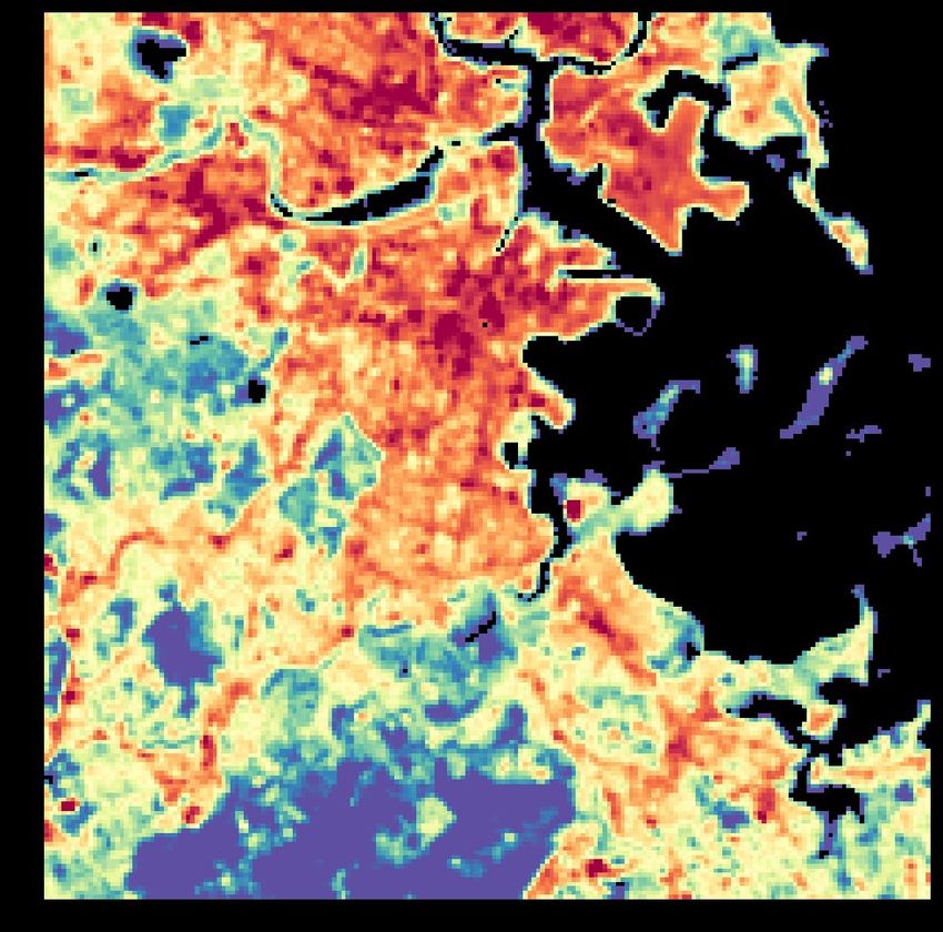
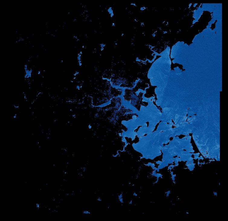
Figure 2: Sample of Sentinel-2 processed data for Normalised Difference Vegetation Index, NDVI (left) and Normalised
Difference Water Index, NDWI (right).

The satellite data is processed into different land cover indices used by the UCM through
processing of different multispectral band combinations to provide LULC conditions such as
Normalised Difference Vegetation Index (NDVI) for vegetation coverage and Normalised Difference
Water Index (NDWI) for water bodies i.e.,
 − 
 = (2)
 + 
 − 
 = (3)
 + 
where NIR, RED and GREEN represent the near infrared, red and green multispectral band data
from Sentinel-2. An example of the processed NDVI and NDWI indices for Boston is shown in
Figure 2.

 9

For urban massing (building heights) building footprint
and elevation data provided by city of Boston (for the
Boston Municipality) was combined with older datasets
for outlying areas to derive a regional building height
map that covers the extents of the model. The building
height data is also averaged into a 100m resolution
raster tile which is used in the model to mathematically
determine the surface sky view factor and hourly shade
fractions, among other things that influences the
localised surface energy balance solution. Hourly shade
fractions at each tile are calculated based on the local
hourly solar position, similar to the methodology of
(Kusaka, 2001).

 Figure 3: Image sample of building footprint and
 height data for the City of Boston

2.3.4 Additional model thermal specification inputs

Additional modelling inputs and assumptions are required by the model where the information is
not provided by the satellite derived LULC tile set, with a selection shown in Table 1.
Table 1: Additional K-UCMv1 land surface specifications

 Ground (soil): Specific thermal heat capacity (kJ/m3/K), thermal conductivity 1900, 0.8, 0.9
 (W/m/K), emissivity

 Walls: Specific thermal heat capacity (kJ/m3/K), thermal conductivity (W/m/K), 1340, 0.8, 0.94, 0.25
 albedo

 Roofs: Specific thermal heat capacity (kJ/m3/K), thermal conductivity (W/m/K) 1400, 0.8, 0.94

2.3.5 UCM Modelling Output - Heat indices

The UCM model produces a data array that represents the spatio-temporal climatic variables
covered within the model region and for the analysis period. The data array represents the
modelled, average hourly urban meteorological condition at 100m spatial resolution. This datasets
is further processed into urban heat indices and delivered as georeferenced image layers (geotiff
rasters) to the design team (Sasaki) for further processing and integration into the overall study
program deliverables. The data layers are resampled to 10m resolution using a bilinear

 10

interpolation. This is done purely for visualisation purposes when overlaying the model data with
other datasets. The key data layers that were processed and integrated into the main report
include:

 • Air Temperature (Ta): The near surface air temperature. Four map layers were produced to
 show the spatial distribution of air temperature across Boston at different time periods on
 the warmest day of the analysis week. These were air temperatures during the night (3am),
 morning (10am), afternoon (3pm) and evening (9pm).

 • Urban Heat Island Intensity (UHII): To better study the temporal effects of the urban heat
 condition an Urban Heat Island Intensity metric was defined, similar to that described in Taha
 et al. (Taha, H. and Freed, T., 2015). The UHII uses the entire weeklong hourly dataset and
 sums the hourly difference between the local and rural air temperature before averaging this
 by day i.e.,
 
 24
 = �( − ) (3)
 
 1

 The index therefore provides a daily degree hours (°F-hr.day-1) index as a measure of the
 overall difference between a local condition and the regional temperature. In effect, the
 degree hour map helps to highlight areas that remain hot and for longer and is therefore
 reflective of both the intensity and the duration of localised heat within the city. The design
 team (Sasaki) have subsequently modified the exported data layer further to show the UHII
 as an average daily temperature difference above the rural temperature.

 • Land Surface Temperature (LST): The surface temperature of the ground at 10am of the
 warmest day during the analysis week. This provides an additional measure of the ground
 surface temperature condition within the urban context at a similar time stamp when Landsat
 8 satellite data is gathered.

 • Heat Event Duration (HED): The heat event duration is the modelled duration (hours)
 during which heat conditions exceed heat advisory levels during the analysis week. The
 Boston heat advisory index determines whether to issue a heat advisory, alert, or emergency
 based on forecasted weather conditions and uses the heat index, as defined by the National
 Weather Service (NOAA, n.d.), to determine the heat event level. In this work the HED is
 calculated as the number of hours during the analysis week that the heat index exceeded a
 threshold temperature of 95°F (heat alert level) for the days when the daytime low
 temperatures did not drop below 75°F. This index useful to determine which neighbourhood
 areas would stay the hottest for the longest during weeks with heat wave events.

 11

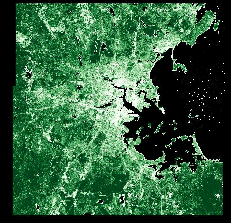
3. Urban Heat Modelling Runs
An analysis domain was selected with an extent of approximately 31km by 31km centred over the
Boston Municipality. For this domain, two different weeklong historical analysis periods were
analysed:

 • The first period selected was for a week of July 10-17, 2016. This sample period coincides
 with a day (July 13, 2016) during which a near cloudless Landsat 8 image was available from
 which a LST surface map could be generated that is independent of the K-UCMv1 derived
 land surface temperatures. The purpose here was to compare the Landsat 8 LST map and the
 K-UCMv1 LST approximation as a measure of the performance of the modelling approach to
 predict surface temperatures.

 • The second period selected was for a week of July 18-24, 2019. This period was chosen in
 collaboration with the City of Boston to model a period that coincided with a reported
 strong heat wave event in the recent past. The analysis results and data layers obtained from
 this modelling period was the main focus and deliverable of the current work. The resultant
 output data layers were integrated and overlayed with additional datasets by the design
 team (Sasaki) as shown and discussed in the main report.

A few key output data layers for the analysis periods are provided as samples below. The raw data
layers were processed and integrated by the design team (Sasaki) into the main Task 2 report that
forms part of the overall Heat Resilience dataset.

3.2 Case Study: July 10-17, 2016
For the current work surface temperature predictions were used to test its performance against
Landsat 8 processed data. The modelled land surface temperature obtained from the K-UCMv1 is
shown here for comparison to the Landsat 8 derived LST in Figure 4. The K-UCMv1 model land
surface temperature map is produced for the same hour during which the Landsat 8 satellite image
was taken, between 10am and 11am on the morning of July 13, 2016. As shown in Figure 4, the
spatial distribution of the warm and cooler surfaces predicted by K-UCMv1 generally seems to
agree with the surface temperature distribution and range found from the Landsat 8 analysis.

 12

Figure 4: Spatial comparison of the LST as modelled by K-UCMv1 (left) and processed from Landsat 8 data (right) for July
13, 2016, at approximately 10am. Temperature scale is in °C.

Figure 5 shows a pixel-by-pixel comparison between the K-UCMv1 model and the Landsat 8
processed land surface temperature data. This suggests that the K-UCMv1 model is capable of
producing similar trends across the analysis region. The correlation between the Normalised
Difference Vegetation Index (NDVI) and the surface temperature is also compared in Figure 5. This
shows that the K-UCMv1 model generally matches the trend of the Landsat 8 surface temperature
variation with NDVI although the Landsat 8 data has more variation across NDVI levels.

The current work and this methodology report do not intend to be a complete validation of the K-
UCMv1 method as this is an on-going effort with continuous modelling approach updates and
improvements. In particular, the K-UCMv1 model is part of an international comparative study to
assess the performance of urban canopy models to predict surface energy fluxes.

 13

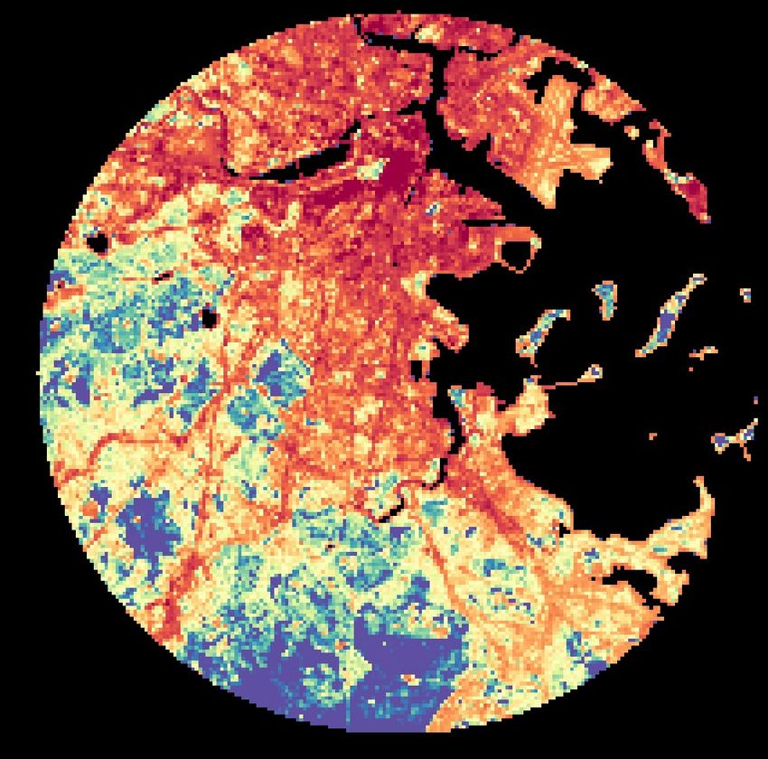
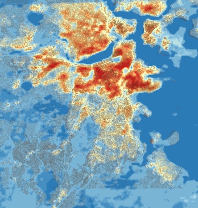
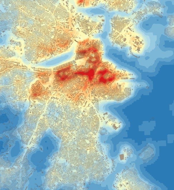
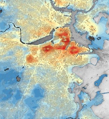
Figure 5: (Left) Correlation between the land surface temperature (°C) modelled by K-UCMv1 and from processed Landsat
8 data for July 13, 2016 10am. (Right) Correlation between the Normalised Difference Vegetation Index (NDVI) and the
predicted land surface temperature from K-UCMv1 and Landsat 8.

3.3 Case Study: July 18-25, 2019
Based on discussions with the City of Boston, a weeklong period of July 18 to 24, 2019 was selected
to produce the heat characteristics maps for the Boston Heat Resilience Study. This week coincided
with a very intense heat wave with peak temperatures of approximately 36°C on July 21 and July 22
measured at the airport. The main output data layer results are discussed in the main report of the
Heat Resilience Study as integrated into the design team deliverable by Sasaki. A sample of the set
of the data layers provided to the design team is shown below only to highlight the different
output data layers with a brief description of the spatial and temporal heat characteristics across
the city. The main design report uses the exported data layers to zoom into specific focus areas
(neighbourhoods) to examine the urban context that may cause elevated high urban heat island
conditions and help identify potential mitigation measures to improve it.

Figure 6 shows a map of the modelled Urban Heat Island Intensity (UHII) index and the Heat Event
Duration (HED) index for the week of July 18 to 24, 2019. The UHII index highlights areas that have
the hottest and longest departure (difference) from the rural temperature condition. This is also
shown in the Heat Event Duration index, which shows that solar exposed neighbourhoods, with
extensive hardscape, massing and limited vegetation, stays within heat wave conditions the longest
(33 to 36 hours) compared to rural outskirts and forested areas that stay within heat wave
conditions the shortest (25 hours) during the analysis week of July 18 to 25, 2019.

 14

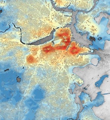
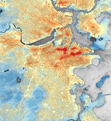
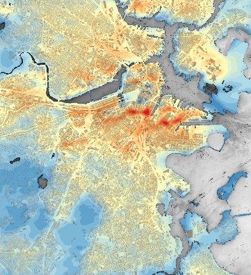
Figure 6: (Left) Urban Heat Island Intensity (°F-hours/day) and (right) Heat Event Duration (Hours/week) for Boston on July
22, 2019.

Figure 7 shows the near surface air-temperature map for July 22, 2019 for four periods during the
day namely night (3am), morning (10am), afternoon (3pm) and evening (9pm). This highlights the
change of air temperature during the course of one day during the very hot conditions of July 20-
22, 2019. Cooler daytime temperatures are modelled for areas within the deeply shaded spaces of
the denser urban centre with its tall massing. Daytime temperatures within solar exposed areas with
significant hardscape are the highest. During night-time, the suburban outskirts cooled down faster
compared to the dense urban core which retains the most heat and becomes the warmest area.
One of the main reasons for warmer temperatures occurring within the city core during the night
and into the early morning, compared to the cooler outlying suburban and forested areas, is the
slower release of heat stored within the urban massing and its land surface. In more exposed areas
the heat is released quickly due to the higher night sky exposure and enhanced open area
ventilation. The comparably warmer night-time and morning temperatures and cooler afternoon
temperatures within the denser urban cores were also found in Portland by Voelkel et al. (Voelkel,
2017).

 15

(a) (b) (c) (d)

Figure 7: Near surface air temperature (°F) on July 22, 2019 for (a) 3am, (b) 10am, (c) 3pm and (d) 9pm

4. Summary
This report highlights the urban canopy modelling methodology used as part of the City of Boston
Heat Resilience Study. It describes the main heat characteristic indices, exported as georeferenced
data layers, employed to help visualise the urban heat characteristics across the Boston Municipality
and in the neighbourhood focus area heat analysis and mitigation work. The final data layer output
and visualisations are provided and discussed in more detail for key Boston neighbourhoods in the
main report by the design team.

 16

References
Barsi, J. S. (2005). Validation of a Web-Based Atmospheric Correction Tool for Single Thermal Band
 Instruments. . Proceedings of Earth Observing Systems X, San Diego, CA., Proc. SPIE Vol. 5882.

ERA5. (2017). Fifth generation of the European Centre for Medium Range Weather Forecasts
 (ECMWF) atmospheric reanalyses of the global climate. Copernicus Climate Change Service
 (C3S) .

Kusaka, H. K. (2001). A simple single-layer urban canopy model for atmospheric models:
 comparison with multi-layer slab models. Boundary-Layer Meteorology, 101:329-358.

Lee, S. a. (2008). A vegeted urban canopy model for meteorological and environmental modelling.
 Boundary-Layer Meteorology, 128:73-102.

NOAA. (n.d.). Heat Forecast Tools. Retrieved from National Weather Service, National
 Oceanographics and Atmospheric Admininstration: https://www.weather.gov/safety/heat-
 index

Oke, T. M. (2017). Urban Climates. Cambridge University Press.

Peng, X. W. (2020). Correlation analysis of land surface temperature and topographic elements in
 Hangzhou, China. Nature Research, Scientific Reports, 10: 10451.

Ryu, Y. B. (2011). A new single-layer urban canopy model for use in mesoscale atmospheric models.
 Journal of applied meteorology and climatology, 50: 1773-1794.

Sentinel-2. (n.d.). Sentinel-2. Retrieved from https://sentinel.esa.int/web/sentinel/missions/sentinel-2

SRTM. (n.d.). Surface Radar Topography Mission. Retrieved from https://www2.jpl.nasa.gov/srtm/

Taha, H. and Freed, T. (2015). Creating and mapping an urban heat island index, California
 Environmental Protection Agency.

Voelkel, J. a. (2017). Towards Systematic Prediction of Urban Heat. Climate, 5, 41.

wikipedia. (n.d.). Penman-Monteith. Retrieved from
 https://en.wikipedia.org/wiki/Penman%E2%80%93Monteith_equation

 17