Temperature Impact on Drinking Water Consumption - MDPI

Proceedings
Temperature Impact on Drinking
Water Consumption †
Dejan Dimkić *
 Jaroslav Černi Water Institute, 11226 Belgrade, Serbia
 * Correspondence: dejan.dimkic@jcerni.rs; Tel.: +381-11-3906478
 † Presented at the 4th EWaS International Conference: Valuing the Water, Carbon,
 Ecological Footprints of Human Activities, Online, 24–27 June 2020.

 Published: 19 August 2020

 Abstract: The production of water in a drinking water supply system (WSS) comprises all drinking
 water enter in the net, while the consumption of water generally comprises all billed amounts of
 water in a WSS. The production and consumption of water in a drinking WSS depend on different
 factors. Consumption rates depend on the consumer structure and habits, industrial demand, time
 of year, water pricing, climatic variables, secondary water losses and many other factors. One of the
 interesting factors is air temperature. It is especially important in the frame of climate change and
 global warming. Temperature impact on water consumption in a WSS is not uniform temporally
 (particularly throughout the year) and spatially (different climate regions and countries, different
 habits and different conditions in each WSS). Obtained correlations for the two biggest cities in
 Serbia (Belgrade and Niš) are presented in the paper and compared with some examples worldwide.

 Keywords: air temperature; water consumption; water supply system; climate change

1. Introduction
 It is well-known that abstracted water in one water supply system (WSS) is the sum amount of
water abstracted by wells, from captured springs and/or by water intake structures. Produced water
in one WSS (in International Water Association - IWA terminology, “entered in a WSS”) is the amount
of water after water treatment. Some other terms are more fluid. Assuming that all flowmeters in a
WSS work properly, and that “authorized unbilled” and “not authorized” consumption are
negligible, the consumed amount of water in one WSS is the amount of water consumed by the
categories (household, industry and city institutions) or by all categories in total. With these
assumptions (relevant for this paper), water production (WP) in a WSS is the compound of the total
water consumption (TWC) or “paid water“ in IWA terminology and primary water losses—in net,
before consumer’s flowmeters (“real losses”). Primarily, water losses vary very much from country
to country (from WSS to WSS in the same country, too) and, generally, are higher in less or medium-
developed countries.
 As noted, the total water consumption is made up of the consumption for household needs,
including the watering of gardens (residential water use, which includes indoor and outdoor activities);
consumption by industry (commercial) and city institution’s consumption (schools, hospitals, etc.),
and vary from less than 50% to more than 90% of water production amounts. Consumption rates
depend on the consumer structure and habits, industrial demand, water pricing, climatic variables,
secondary water losses and many other factors, including the specific condition of any particular WSS.
 Regarding the consumption pace of change, socioeconomic variables such as population,
income, the price of water, housing characteristics, etc. can impose medium-term or long-term
changes in water consumption patterns, while climatological variables such as precipitation and
temperature induce short-term changes [1].

Environ. Sci. Proc. 2020, 2, 31; doi:10.3390/environsciproc2020002031 www.mdpi.com/journal/environsciproc

Environ. Sci. Proc. 2020, 2, 31 2 of 12

 The impact of climatic parameters is not uniform temporally (particularly throughout the year)
and spatially (different climate regions and countries and different habits). Geographic locations with
cold winters and warm summers are especially sensitive. In such locations, two water consumption
segments occur in the year: the warm part (spring-summer) and winter [2]. Cold temperatures,
freezing precipitation and snow-covered ground surfaces, for example, tend to restrict water use to
indoor activities in the winter. On the other hand, spring-summer warm temperatures and snow-free
ground surfaces may induce significant increases in water consumption, both indoors and outdoors
[3]. The main investigated climatic variables in the literature are temperature and precipitation, but
others, such as wind or relative humidity or evaporation, also affect spring-summer water use. In a
majority of cases, they are not considered because of the unavailability of data.
 It would have been interesting to investigate different types of consumption as a function
of the climatological variables, but the needed data are not available generally. More important
(especially due to climate change) is how much the increase of temperature, or changes in
precipitation, affect the TWC or WP in a WSS. The topic of this paper is the air temperature (T) impact
on the TWC (or WP). Several examples of this impact are presented. It is not fully clear in these
examples if some authors by the term “water consumption” maybe mean “water production”
(this paper’s author’s remark).

2. Air Temperature Impact on Water Production in the Cities of Belgrade and Niš, Both in Serbia
 Only daily averages during the warmer part of the year, from May to October, were analyzed.
Given certain specific features of each of these months (varying uses of water for gardening, summer
holidays, etc.), they were grouped into three periods that are analyzed and presented separately:
(1) May and June, (2) July and August and (3) September and October. A linear trend was determined
for each plot, and the respective equation and coefficient of determination were graphically
represented. Then, the percent change in water production for the difference of 1 °C was computed [4].

2.1. Belgrade
 A public water supply in Belgrade began in 1892 with some 40 L/s withdrawn from springs
within the city and its environs for the 50,000 inhabitants at that time. Production peaking was at the
beginning of the 21st century at an overall annual average rate of 7.5 m3/s. The efficiency of the system
has been upgraded considerably in period 2002–2012 (Table 1), such that the annual average
production rate is up to 6.5 m3/s (200 million m3/year). Today, in the Belgrade WSS, six water
treatment plants processed abstracted water. A distribution network that is some 3500-km-long
delivers water to about 1.5 million inhabitants and numerous industries and institutions.

 Table 1. Total water production in the Belgrade water supply system (WSS) in 2002 and from 2008 to
 2012 year.

 Year 2002 2008 2009 2010 2011 2012
 Total water production (Mil. m3/year) 233 218 214 203 202 201

 Figure 1, from (a) to (c), shows the correlation between the total water production in the Belgrade
WSS and recorded daily temperatures for the months May/June, July/Aug and September/October
during 2011–2013. Then the percent variation in the production rates (rate of WP) for 1 °C is computed.

Environ. Sci. Proc. 2020, 2, 31 3 of 12

 7500
 y = 46.359x + 5420.4
 7000 R2 = 0.502

 Average daily production (l/s)
 6500

 6000

 5500

 5000

 4500

 4000
 0,0 5,0 10,0 15,0 20,0 25,0 30,0 35,0
 Average daily tem perature (°C)

 (a) May and June (Taver. = 20.2 °C)

 7500

 7000 y = 51.346x + 5292.6
 Average daily production (l/s)

 R 2 = 0.4086
 6500

 6000

 5500

 5000

 4500

 4000
 0 5 10 15 20 25 30 35
 Average daily tem perature (°C)

 (b) July and August (Taver. = 25.0 °C)

 7500

 7000
 Average daily production (l/s)

 6500

 6000

 5500
 y = 7.4565x + 6347.8
 5000 R 2 = 0.0242

 4500

 4000
 0 5 10 15 20 25 30 35
 Average daily tem perature (°C)

 (c) Sep. and Oct. (Taver. = 20.2 °C)

 Figure 1. The Belgrade water supply system (WSS): correlation between the average daily water
 production (WP) and average daily temperature (T) (2011–2013).

May and June:
 46.359 • 100
 = • 1 °C = 0.73% (1)
 6358

July and August:
 51.346 • 100
 = • 1 °C = 0.78% (2)
 6577
September and October:
 7.4565 • 100
 = • 1 °C = 0.11% (3)
 6499
 The highest average water production rate in Belgrade was recorded, as expected, in the
warmest summer months, July/August (6577 L/s), followed by September/October (6499 L/s).

Environ. Sci. Proc. 2020, 2, 31 4 of 12

The lowest was registered in the May/June (6358 L/s) months of the study period. The variation in
WP as a function of T was similar in May/June and July/August, while it was much lower in
September/October.

2.2. Niš
 The city of Niš and its surroundings (total population about 260,000) receive drinking water
from the regional WSS, called NIVOS. NIVOS comprises several different sources, about 30 pumping
stations, some 30 water tanks, roughly 100 km of water mains and approx. 800 km of service pipes.
 Water production and delivery have been continuously metered since 2003 (Table 2—total and
Figure 2—by categories). Based on these data, NIVOS has provided about 1190 L/s on average.

 Table 2. Average yearly total water production in NIVOS from 2003 to 2010.

 Year 2003 2004 2005 2006 2007 2008 2009 2010
 Average yearly production (L/s) 1268 1219 1201 1250 1203 1156 1158 1166

 The water supply has generally been stable in terms of quantity and quality (drinking water
standards). Since 2003, water losses have varied from 36% to 43%. The proportions by consumer
categories were: households 41%, industries and institutions 19% and unbilled consumption 40%.

 Produced and billed water (mil. m3 )
 Households Industry, businesses and institutions
 Total billed Total produced (m3)
 50
 Volume ( mil. m3 )

 45
 40
 35
 30
 25
 20
 15
 10
 5
 0
 2003 2004 2005 2006 2007 2008 2009 2010

 Figure 2. NIVOS: Annual production and billed consumption rates by user category (2003–2010).

 Figure 3, from (a) to (c), shows the correlation between the total water production and recorded
daily temperatures for the months May/June, July/August and September/October during 2003–2010
at NIVOS. Then the percent variation in the production rates (rate of WP) for 1 °C is computed.

Environ. Sci. Proc. 2020, 2, 31 5 of 12

 1700
 y = 11.106x + 995.42
 1600 2
 R = 0.2724

 Average daily production (l/s)
 1500

 1400

 1300

 1200

 1100

 1000

 900
 0 5 10 15 20 25 30 35

 Average daily tem perature (°C)

 (a) May and June (Taver. = 19.4 °C)
 1700
 y = 12.64x + 969.13
 1600 2
 R = 0.3183
 Average daily production (l/s)

 1500

 1400

 1300

 1200

 1100

 1000

 900
 0 5 10 15 20 25 30 35
 Average daily tem perature (°C)

 (b) July and August (Taver. = 23.0 °C)
 1700
 y = 4.8148x + 1127.1
 1600
 2
 R = 0.1564
 Average daily production (l/s)

 1500

 1400

 1300

 1200

 1100

 1000

 900
 0 5 10 15 20 25 30 35
 Average daily tem perature (°C)

 (c) Sep. and Oct. (Taver. = 14.8 °C)

 Figure 3. NIVOS: correlation between the average daily WP and average daily T (2003–2010).

May and June:
 11.106 • 100
 = • 1 °C = 0.92% (4)
 1211
July and August:
 12.64 • 100
 = • 1 °C = 1.00% (5)
 1260
September and October:
 4.8148 • 100
 = • 1 °C = 0.40% (6)
 1199
 The highest average rate of water production at NIVOS was also recorded in the warmest
summer months—July/August (1260 L/s), followed by May/June (1211 L/s). The lowest was
registered in the months September/October (1199 L/s). The variation in WP as a function of T was
similar for May/Jun and July/August, while it was again much lower in September/October.
 In July/August, both systems recorded the highest average rates of WP, despite temporarily
reduced populations. This is attributed to higher T during this period relative to the other two.
NIVOS recorded a higher WP in May/June than in September/October, to which the watering of
gardens was a contributing factor during this period. Belgrade reported a higher WP in

Environ. Sci. Proc. 2020, 2, 31 6 of 12

September/October than in May/June as a result of a higher population count, while the average daily
T were the same for the two periods (20.2 °C).
 The slopes of the trend lines show that both systems exhibited a greater impact of T on the WP
during the first two periods: May/June and July/August. As previously suggested, this was due to
the watering of gardens and other green surfaces (even they are not too high) to a much greater extent
than in the third period, September-October. For the first two periods, it appears that a T increase of
1 °C causes an average increase in the rate of WP of approximately 1%.

3. Air Temperature Impact on Water Consumption Worldwide—Examples

3.1. Example: The City of Calgary—Alberta (Canada)
 The city of Calgary (approx. 1.4 million inhabitants) exhibits an impressive climate variability
throughout the year [3]. The city has a cold climate, with a strong T contrast between day and night,
as well as winter and summer. The summers are cool, with a mean daily T of 15 °C. Temperatures
during the summer have the least variability and rarely exceed 32 °C. The primary objective was to
examine the effects of the mean maximum weekly T on the weekly TWC per capita in the spring-
summer season. The summer TWC per capita tends to be higher and, in some cases, is twice as much
as the winter water use.
 Figure 4 shows a plot of the mean maximum weekly T and weekly TWC per capita from January
1982 through December 1989. Two distinct segments can be discerned. The weekly TWC per capita
seems to be fairly steady when the mean maximum weekly T is below 15 °C. In contrast to that,
the TWC per capita increases with the increasing mean maximum weekly T when temperatures
exceed 15 °C.
 Weekly Water Consumption Per Capita
 (ML)

 Mean maximum Weekly Temperature (Celsius)

 Figure 4. Weekly water consumption per capita and mean maximum T, January 1982—December
 1989, for Calgary.

 If a trend line would be put in Figure 4 for temperatures above 15 °C, the slope would show that
T increases of 1 °C cause an average increase in the rate of the TWC of approximately 4%:
 For T = 15 °C, the average weekly consumption per capita is approx. 430 ML.
 For T = 30 °C, the average weekly consumption per capita is approx. 700 ML.
 700 ML − 430 ML 1 °C
 = • • 100% = 4.19%/1° (7)
 430 ML 30 °C − 15 °C
 Figure 4 demonstrates also that the weekly TWC per capita during the winter is virtually
insensitive to changes in the mean maximum weekly T. Consumption sensitivity begins when the
temperature exceeds 15 °C, and this normally begins from May, when the mean monthly maximum
temperature is 16 °C.

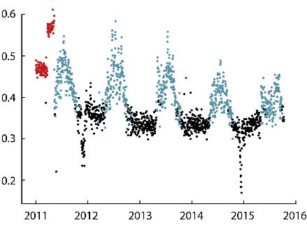
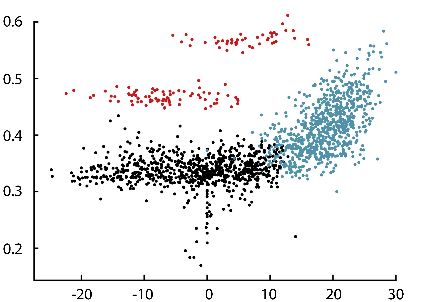
Environ. Sci. Proc. 2020, 2, 31 7 of 12

3.2. Example: The City of Montreal (Canada)
 In the analyses of the observed drinking water consumption of the city of Montreal
(approx. 1.8 million inhabitants), a clustering analysis of the daily data of the TWC and T were
used [5]. It is proposed to split the observations of the daily TWC (period 2011–2016) into two main
clusters (black and blue colors) and, additionally, some no-standard data in a separate cluster
(red color). This choice is simple and works well to separate the base water use from the seasonal
water use (Figure 5a,b).
 Daily water consumption q

 Daily water consumption
 q (m3/(capita.day))
 (m3/(capita.day))

 (a) (b)

 Figure 5. (a) observations of daily total water consumption (TWC) and (b) scatter plot of the daily
 Table 12. °C) for the occurrences of transition from the base to seasonal TWC and vice versa. It is
 acceptable to treat the base water use as independent of T, but the use is subject to weekday/weekend
 effects. The seasonal water use depends on the daily minimum and maximum T and daily total
 precipitation (not presented here).

 If a trend line would be put in Figure 5b for T above 12 °C, the slope would show that T increases
of 1 °C cause an average increase in the TWC of approximately 3%:
 For T = 12 °C, the average daily consumption per capita is approx. 0.35 m3 = 350 L/per capita/
per day.
 For T = 27 °C, the average daily consumption per capita is approx. 0.50 m3 = 500 L/per capita/
per day.
 500 L − 350 L 1 (8)
 = • • 100% = 2.86%/1 °C
 350 L 27 °C − 12 °C

3.3. Example: The City of Seoul (South Korea)
 The relation between the daily weather variables and TWC were examined in the case study of
the South Korea capital Seoul (app. 9.8 mil. inhabitants) [6]. Figure 6a shows the observed average
monthly precipitation and T, and Figure 6b shows the monthly TWC per capita in Seoul in the period
2002–2007.
 Average precipitation (mm)

 Per capita water use (CM)

 (a) (b)

 Figure 6. (a) Average monthly T and precipitation and (b) the TWC per capita, by months
 (2002–2007).

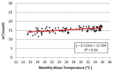
Environ. Sci. Proc. 2020, 2, 31 8 of 12

 Similar to the majority of studies that investigate T impacts on the TWC, they found that the
average daily T and maximum daily T are good predictors of the TWC (Figure 7a,b).
 Water use (mil. CM.)

 (a) (b)

 Figure 7. Summer water use and (a) mean daily T, and (b) maximum daily T in Seoul (2002–2007).

 If it is calculated, the TWC base on the trend line in Figure 7a for temperatures above 15 °C,
the slope would show that T increases of 1 °C cause an average increase in the rate of the TWC of
approx. 1%:
 For T = 15 °C, the average daily water use is 3.46 million CM
 For T = 30 °C, the average daily water use is 3.94 million CM.
 3.94 mill. CM − 3.46 mill. CM 1
 = • • 100% = 0.85%/1 °C (9)
 3.46 mill. CM 30 °C − 15 °C

 Very close results would be obtained if the TWC was calculated as the impact of the maximum
T (Figure 7b) or based on the monthly averages from Figure 6a,b.

3.4. Example: Bahrain
 The urban water management in Bahrain is under major stress and is being influenced by a
multitude of driving forces, such as high population growth and urbanization rates, high water
consumption per capita, high water losses and the limited availability of water resources [7].
 Observed data from the period 2005–2011 show an increase in monthly water consumption with
increasing monthly mean temperature (Figure 8).

 Figure 8. Correlation between the monthly mean T and monthly TWC per capita (2005–2011).

 Climate changes additionally press this already stressed system. An assessment of the
vulnerability of the municipal water management system to the impacts of climate changes (CC) in
the future have been done, and results are presented on Figure 9.

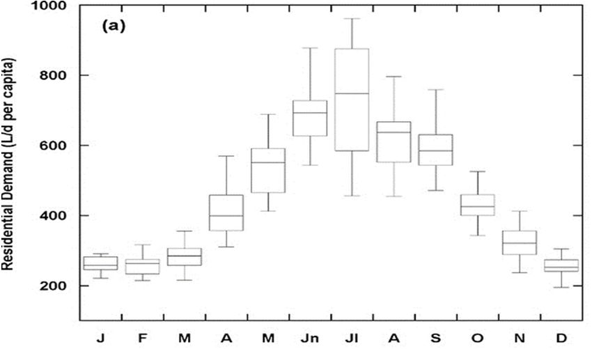
Environ. Sci. Proc. 2020, 2, 31 9 of 12

 Figure 9. Projected impact of the additional TWC in Bahrain due to the prediction of T increases
 (2011–2030).

 The rate of water consumption for T increases of 1 °C could be calculated based on the trend line
in Figure 8. For T between 16 °C and 36 °C, the slope shows that T increases of 1 °C cause an average
increase in the rate of the TWC of approx. 1%:
 For T = 16 °C, the average monthly TWC per capita is 14.0 m3.
 For T = 36 °C, the average monthly TWC per capita is 16.5 m3.
 16.5 − 14.0 1
 = ⋅ ⋅ 100% = 0.89%/1 °C (10)
 14.0 36 °C − 16 °C

3.5. Example: The Cities of Portland (Oregon) and Albuquerque (New Mexico), Both in the USA

3.5.1. Portland (Oregon—USA)
 The city of Portland (approx. 0.7 million inhabitants) has water consumption that exhibits
seasonal patterns (Figure 10a). During the wet, cooler period (November to April), the monthly
average TWC is constant and low, with the lowest TWC occurring in February. During the dry,
warm period (May to October), the monthly average TWC is high. The average monthly TWC of July,
the peak month, is approximately two-thirds (66%) higher than that of February. The TWC during
the summer months (from June to September) is nearly 41% of the annual TWC [8].
 Average Temperature (⁰ C)
 Average annual per capita
 consumption ( L / day )

 (a) (b)

 Figure 10. (a) Distribution of the monthly TWC (L/day/per capita) and average max. T (°C) and
 (b) T impacts on the TWC from April to October in Portland (1960–2013).

 When the trend is put on (Figure 10b) for the months April-October, the slope shows that T
increases of 1 °C cause an average increase in the rate of water consumption of approx. 5%:

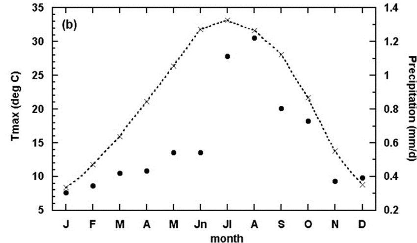
Environ. Sci. Proc. 2020, 2, 31 10 of 12

 For T = 16 °C, the average daily consumption per capita is approx. 500 L.
 For T = 28 °C, the average daily consumption per capita is approx. 820 L.
 820 L − 500 L 1
 = • • 100% = 5.33%/1 °C (11)
 500 L 28 °C − 16 °C

3.5.2. Albuquerque (New Mexico—USA) [9]
 The water use in Albuquerque—New Mexico (approx. 0.6 million inhabitants) increases
dramatically during the summer, principally due to increased outdoor water use [9]. Instead of the
TWC, the residential water demand was correlated with the monthly average maximum T (Figure 11).
 Residential use makes up, on average, 60% of the municipal, publicly supplied water in the USA
[10]. It can be divided into base use, defined primarily as the indoor use lowly dependent of the
influence of climate, and seasonal use, which is significantly climate-dependent. Seasonal water use
refers to the mostly outdoor summer water use and, together with the climatically insensitive base
use, makes up the total water use.
 The outdoor water use can account for 22–65% of the annual residential use [11] and includes
landscape irrigation, swimming pools, refreshing concrete surfaces and car washing. Depending on
the fraction of municipal use that is used outdoors, as well as other potentially weather-sensitive uses
of municipal water, such as commercial or institutional outdoor irrigation and water used in heating
and cooling, the municipal water use is affected to varying degrees by the weather.
 When the trend is put on (Figure 11c) for the months April-October, the slope shows that T
increases of 1 °C cause an average increase in the rate of the WP of approx. 7%:
 For T = 21.5 °C, the average daily consumption per capita is approx. 400 L.
 For T = 32.5 °C, the average daily consumption per capita is approx. 700 L.
 700 L − 400 L 1
 = • • 100% = 6.82%/1 °C (12)
 400 L 32.5 °C − 21.5 °C

 Figure 11. (a) Residential demand (L/day/per capita) by months, (b) average of the T maximum and
 average daily precipitation by months and the (c) Tmax impact on the TWC from April to October,
 1980–2001.

Environ. Sci. Proc. 2020, 2, 31 11 of 12

4. Discussion and Conclusions
 Water use (synonym for total water consumption—TWC) is influenced by a diverse set of
climatic, socioeconomic, demographic, policy and landscape factors. Climatic variables could be the
temperature (maximum daily, average daily, average monthly and minimum daily); precipitation
(amount, frequency and duration); soil humidity; wind (speed intensity, frequency and duration); etc.
In addition to climatic, the most important variables are demographic changes, the availability of water
resources, income, the price of water, the WSS characteristics, people’s habits and several others.
 Temperature impacts on the amount of drinking water consumption (or production) is the topic
of this paper, with a focus on the percent of changes in the TWC (or WP) due to increases in the T.
Even though consumption and production are not the same parameters, they are comparable due to
their reactions to T increases in one WSS being almost the same. Different results are obtained for
different regions in the world. Temperature and precipitation are the most used variables, since data
are widely available and highly explanatory, particularly for estimating seasonal or summer-isolated
water uses. In general, an increased TWC is related to a higher T and lower precipitation [9,12].
 The daily base use could be sensitive to the days of the week, and daily seasonal uses exhibit a
relation to certain temperature thresholds. Examples from the USA and Canada told us that the first
threshold value is about 14 °C and can vary ±2 °C from WSS to WSS. Below this threshold, water use
(base use) is almost independent of the T. Between the first and second threshold (approx. 30 °C, also
±2 °C from WSS to WSS), changes in water use as an impact of the T can be shown enough good
linearly. Changes in water consumption at very high average daily temperatures, above the second
threshold, can be much more severe (in some cases, even exponential dependency can occur) than
below that value [13].
 Temperature impacts on drinking water consumption for the spring-summer months
(average daily temperatures between 14 °C and 30 °C) in the analyzed examples vary; T increases of
1 °C cause an average increase in the TWC from 1% (Serbia, South Korea and Bahrain) through 3%
to 5% for cities in the USA and Canada. A noted extreme of 7% in New Mexico, USA is higher, likely
due to that, in this town, the residential use was correlated instead the TWC. Higher impacts in the
USA and Canada could be attributed to generally higher water availability and lower water losses,
as well as a higher standard.
 It should be concluded that the rate of the above correlations (temperature ÷ drinking water
consumption), in addition to other climate parameters, depend on the water resource availability,
water policy, water supply system conditions and habits of the people in such regions.
Funding: Funded by the Ministry of Education and Science of the Republic of Serbia.

Acknowledgments: To the National scientific project “Assessment of Climate Change Impact on Water
Resources in Serbia” (TR37005), funded by the Ministry of Education and Science of the Republic of Serbia.

Conflicts of Interest: The author declares no conflicts of interest.

References
1. Miaou, S.P. A Class of Time Series Urban Water Demand Models with Nonlinear Climatic Effects.
 Water Resour. Res. 1990, 26, 169–178.
2. Weber, J.A. Forecasting Demand and Measuring Price Elasticity. Am. Water Works Assoc. J. 1989, 81, 57–65.
3. Akuoko-Asibey, A.; Nkemdirim, L.C.; Draper, D.L. The impacts of climatic variables on seasonal water
 consumption in Calgary, Alberta. Can. Water Resour. J. 1993, 18, 107–116, doi:10.4296/cwrj1802107.
4. Dimkić, D.; Slimak, T.; Radenković, Z. Correlation Between Average Daily Temperatures and Production of Water
 in Water Supply Systems; International Conference Climate Change Impacts on Water Resources: Belgrade,
 Serbia, 2013; pp. 153–160, ISBN 978-86-82565-41-3.
5. Rasifaghihi N.; Li S.S.; Haghighat, F. Forecast of urban water consumption under the impact of climate
 change. Sustain. Cities Soc. 2020, 52, 101848, doi:10.1016/j.scs.2019.101848.
6. Praskievicz, S.; Chang, H. Identifying the Relationships between Urban Water Consumption and Weather
 Variables in Seoul, Korea. Phys. Geog. 2009, 30, 324–337, doi:10.2747/0272-3646.30.4.324.

Environ. Sci. Proc. 2020, 2, 31 12 of 12

7. Al-Zubari, W.K.; El-Sadek, A.A.; Al-Aradi, M.J.; Al-Mahal, H.A. Impacts of climate change on the
 municipal water management system in the Kingdom of Bahrain: Vulnerability assessment and adaptation
 options. Clim. Risk Manag. 2018, 20, 95–110.
8. Gato, S.; Jayasuriay, N.; Roberts, P. Temperature and rainfall thresholds for base use urban water
 consumption modeling. J. Hydr. 2007, 337, 364–376.
9. Gutzler, D.S.; Nims, J.S. Interannual Variability of Water Demand and Summer Climate in Albuquerque,
 New Mexico. J. Appl. Meteor. Clim. 2005, 44, 1777–1787, doi:10.1175/JAM2298.1.
10. Dieter, C.A.; Maupin, M.A.; Caldwell, R.R.; Harris, M.A.; Ivahnenko, T.I.; Lovelace, J.K.; Barber N.L.;
 Linsey, K.S. Estimated Use of Water in the United States in 2015; USGS Numbered Series; U.S. Geological
 Survey: Reston, VA, USA, 2018.
11. DeOreo, W.B.; Mayer, P.W.; Dziegielewski, B.; Kiefer, J.; Water Research Foundation. Residential End Uses
 of Water, Version 2; Water Research Foundation: Denver, CO, USA, 2016.
12. Kenney, D.S.; Goemans, C.; Klein, R.; Lowrey, J.; Reidy, K. Residential Water Demand Management:
 Lessons from Aurora, Colorado. J. Am. Water Resour. Assoc. 2008, 44, 192–207.
13. Maidment, D.R.; Miaou, S.-P. Daily Water Use in Nine Cities. Water Resour. Res. 1986, 22, 845–851.

 © 2020 by the authors. Licensee MDPI, Basel, Switzerland. This article is an open access
 article distributed under the terms and conditions of the Creative Commons Attribution
 (CC BY) license (http://creativecommons.org/licenses/by/4.0/).