INTERPRETABLE DEEP NEURAL NETWORK MODELS: HYBRID OF IMAGE KERNELS AND NEURAL NET-WORKS - OpenReview
←
→
Page content transcription
If your browser does not render page correctly, please read the page content below
Under review as a conference paper at ICLR 2020

I NTERPRETABLE D EEP N EURAL N ETWORK M ODELS :
H YBRID OF I MAGE K ERNELS AND N EURAL N ET-
WORKS

 Anonymous authors
 Paper under double-blind review

                                           A BSTRACT
         We introduce interpretable components into a Deep Neural Network (DNN) to
         explain its decision mechanism. Instead of reasoning a decision from a given
         trained neural network, we design an interpretable neural network architecture
         before training. Weight values in the first layers of a Convolutional Neural Net-
         work (CNN) and a ResNet-50 are replaced by well-known predefined kernels such
         as sharpening, embossing, color filters, etc. Each filter’s relative importance is
         measured with a variant of the saliency map and Layer-wise Relevance Propaga-
         tion (LRP) proposed by (Simonyan et al., 2014; Bach et al., 2015). We suggest
         that images processed by predefined kernels still contain enough information for
         DNNs to extract features without degrading performances on MNIST, and Ima-
         geNet datasets. Our model based on the ResNet-50 shows 92.1% top-5 and 74.6%
         top-1 accuracy on the ImageNet dataset. At the same time, our model provides
         three different tools to explain individual classification and overall properties of
         a certain class: the relative importance scores with respects to (1) each color, (2)
         each filter, and (3) each pixel of the image.

1   I NTRODUCTION
A Neural Network (NN) is a nonlinear and complex system with countless configurations. Tracing
and analyzing these networks are extremely difficult but a necessary task to ensure the reliability of
DNNs in critical areas like Pharmaceutics, Finance, and criminal justice. Furthermore, comprehen-
sions on the DNN’s decision-making processes can promote the design of an optimal NN model for
a given data set.
In the previous literature, an interpretation of an NN model is mostly based on trained models.
Obtaining parameters, weights and biases from trained NN models, features (subsets of inputs) are
extracted based on relative importance scores. Although these methods can successfully identify
important features, it is still difficult to tell why such a selection has been made. For example,
Figure 1 shows ‘gradient × input’ scores based on (Shrikumar et al., 2016; Bach et al., 2015). Red
dots imply high scores, but they do not explain how and why these dots are important.
On the other hand, DNNs are highly flexible. Numerous different types of data can be fed
into the NN: RGB, YCbCr, grayscale in different color spaces, the Discrete Cosine Transformed
(DCT)(Lionel et al., 2018) of frequency domain representation, the scale-invariant feature trans-
formed (SIFT)(Liang et al., 2016), bag-of-feature (BoF) model (Brendel & Bethge, 2019), and so
on. DNNs still can be trained to extract features from these different forms of data, but it is not
completely understood how. We believe that the flexibility of DNNs also can be used to explain
classification mechanisms. If we input several different images - processed differently from a single
image - into DNNs and measure how frequently or significantly each image is used, we can deduce
which features or characteristics are used for classification.
In this paper, we propose interpretable DNN architectures called General Filter Neural Net (GFNN)
and General Filter ResNet (GF-ResNet). We introduce human-interpretable components into a
DNN: well-known image kernels such as edge detection, sharpening, embossing, etc. as shown
in Table 1. Figure 1 (a) and (b) depict some of these filters and their effects on the original image.
We substitute the weights of the first layers of a CNN and a ResNet-50 with these filters. Filtered

                                                  1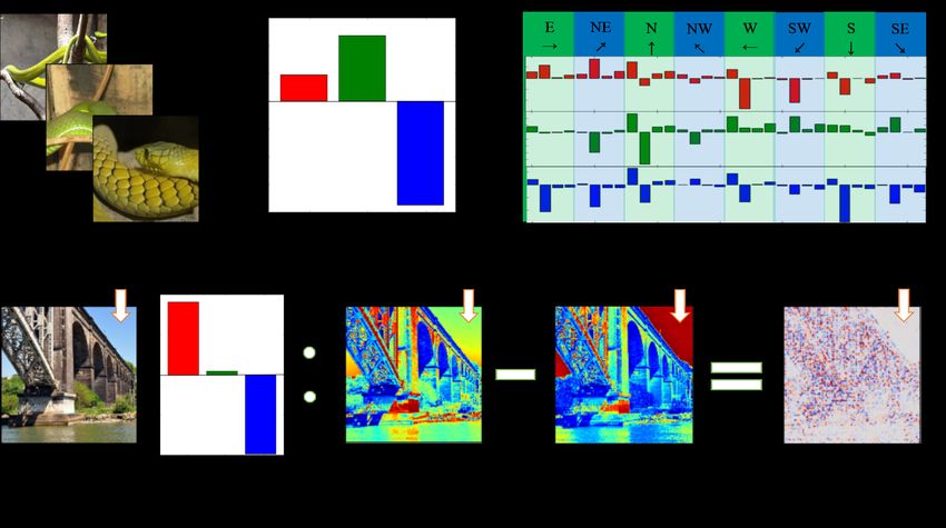
Under review as a conference paper at ICLR 2020

Figure 1: Left. The interpretable neural network model divides input images into several pieces.
Each piece is fed into subsequent networks. (a) Schematic images of the 7th , 15th , 23rd and 31st
filters of GFNN. (b) Each filter is convoluted onto the original images. (c) The filter scores images
as defined in Section 2.1.3, i.e., the gradient × L2 layer. Right. A relative importance can be traced
by several interpreting methods.; Saliency map, gradient × input , and the sum of filter score images
with respect to the input pixels.

by the kernels, a set of transformed images are generated from the input images and they are fed
into the subsequent neural networks. We train the neural network and measure relative importances
of each kernel by a method, based on saliency map and Layer-wise Relevance Propagation (LRP)
(Simonyan et al., 2014; Bach et al., 2015), which will be described in Section 2.

2     F ILTER S CORES AND F ILTER S CORE I MAGES
Our interpretable model is based on two previous feature extraction methods: the saliency map and
LRP (Simonyan et al., 2014; Bach et al., 2015). These approaches were focused on the importance
scores of the input image pixels. Simonyan et al. proposed that the gradient of output layers w.r.t.
pixels of a specific input reflects the relative importance of each pixel (Simonyan et al., 2014). The
magnitude of the gradients indicates the change of which pixels in an input influence most in the
class scores. On the other hand, Bach et al. suggested a method for propagating the importance
scores through layers called LRP (Bach et al., 2015). LRP approach also provides the importance
scores w.r.t. each pixel of an input image. The magnitude of the LRP scores indicates the contri-
butions to the class of each pixel in the image positively or negatively. Shrikumar et al. showed
that the LRP approach is equivalent to the element-wise product of the saliency map and the input
(Shrikumar et al., 2016).
Even though previous approaches were developed independently, they are closely related to each
other. Especially, when the activation function is a piece-wise linear function, saliency map and
LRP approach are rooted in the same equation. In this section, we will (1) discuss the mathematical
relation between the saliency map and the importance scores in LRP, and (2) show that their methods
can be generalized to any layers to monitor important nodes.

2.1     P IECE - WISE L INEAR N EURAL N ETWORK

In this section, we will define a trained neural network model mathematically. The basic assump-
tion of this work is that the activation functions for NN models are Rectified Linear Units (ReLU)
functions. ReLU (x) is linear if x ≥ 0, but is equal to 0 if x < 0. In other words, ReLU (x) is a
piece-wise linear function. We will show the mathematical relations between the piece-wise linear
function and the saliency map and importance scores in LRP.

2.1.1    F RAMEWORK
                                                           l
For a given neural network model M with (nl + 1) layers, wi,j denotes the weight from the ith node
in the l layer to the j node in the (l + 1) layer, and Li and bli denote the ith node (or its value)
        th             th                  st            l

                                                  2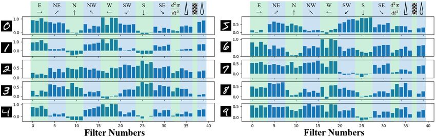
Under review as a conference paper at ICLR 2020

Figure 2: (a) The architecture of GFNN for grayscale images. The difference between a regular
CNN and our model is the substitution of the kernels in the first layer by predefined ones. (b) Our
interpretable components for color images. Predefined kernels are applied to each color components
and resulting layers are concatenated. 1×1×96×D filters, not predefined, are convoluted to reduce
the dimension.

Table 1: List of filter types and their corresponding filter numbers. The first order derivatives filters
are used only when it is indicated. Full list of filters can be found in Appendix
         Kernel Types                Filter Numbers         Kernel Types               Filter Numbers
   Edge Detecting East               0-3                    Second Order Derivative    32, 33
                   Northeast         4-7                    Sharpening                 34-36
                   North             8-11                   Embossing                  37
                   Northwest         12-15                  Blurring                   38, 39
                   West              16-19                  First Order Derivative*    40-47
                   Southwest         20-23
                   South             24-27
                   Southeast         28-31

and the ith bias in the lth layer respectively. Especially, let L0 and Lnl be the input layer and the
output layer with dimensions of nin and nout respectively. All indices such as l, i, j, nin , nout , and
nl are integers.
If rectified linear units function, ReLU(x), is the activation function for an NN model M , then the
value of a node Ll+1j   is
                                                                         !
                                                 X
                                 l+1                    l     l      l+1
                                Lj = ReLU            (wi,j · Li ) + bj                           (1)
                                                    i
                                                                               l
by the definition of artificial neurons. Observe that even though the weights wi,j are a constant for
a trained model M , Lli is a variable, dependent on an input I.
We also denoted MI as the state when an input I is fed into a trained model M . The difference
between M and MI is that while M is a structure, MI is a snapshot of M with the nodes of Llj
loaded with their values from the input I.

2.1.2   O UTPUT L AYERS WITH R ESPECT TO I NPUT L AYER
For an NN model MI , the first layer is the input layer, i.e., L0i = Ii for i = 0, . . . , nin . Similarly,
the output layer is the last layer, i.e., Lnj l = Oj , where Oj denotes the j th node in the output layer
where 0 ≤ j ≤ nout . Jung et al. showed that for any NN models MI ,
                                                 X
                                          Oj =      (αi,j · Ii ) + cj                                  (2)
                                                i

where αi,j , and cj are constants within a polytope-shape partition defined by the ReLU functions
of each node in each layer (Jung et al., 2019). Equation 2 shows that the output layer of an NN is a
piece-wise linear function of the input layer. Specifically,
                                                 P           each parameter to ReLU function defines
a half-space in the input space I such that {Ii : i (αi,j · Ii ) + cj ≥ 0} and their intersections define

                                                        3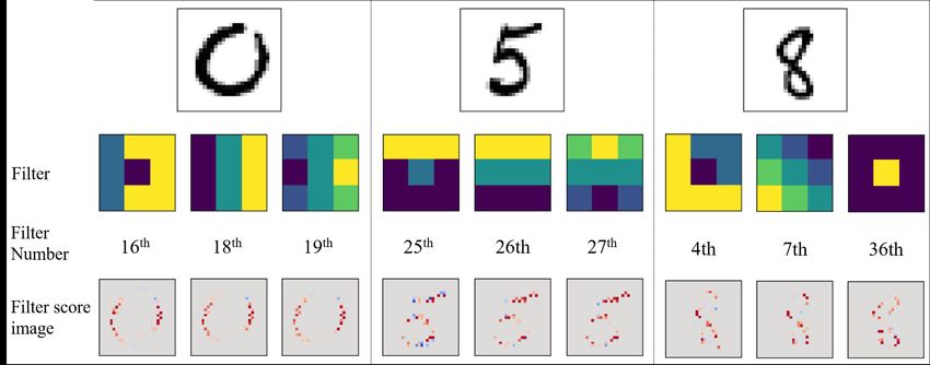
Under review as a conference paper at ICLR 2020

a polytope n, the input space. Because αi,j and cj are constants within each polytope, the output
layer of an NN is a piece-wise linear function of the input layer.
The coefficients, αi,j , are Simonyan et al.’s gradients w.r.t. the input pixels. Similarly, multiplication
of coefficients and pixels of an input, αi,j · Ii , are the same as the scores calculated by LRP or the
gradient × input.

2.1.3   F ILTER S CORES

We generalize importance scores such that they are defined for any layers of an NN. We will define
the importance scores of the first layer in a CNN as filter scores since they imply how important
each filter is.
Proposition 1. For any NN models MI and any l,
                                       X
                                  Oj =    (αi,j · Lli ) + cj                                           (3)
                                                i

where αi,j and cj are some constants.
It is not difficult to prove the proposition since we can substitute Lli for Ii in Eqaution 2 without loss
of generality. Using Proposition 1, we can define the scores similar to the gradient and the gradient
× input for any layer. We define filter scores as the sum of each kernel’s importance scores, i.e.
αi,c · L1i , where c is the largest nodes of the output layer. For example, if a DNN classifies an image
as
P 0, then the filter     score for filter number 37, e.g. an embossing kernel in our model, is given by
                    1
    i∈K (α  i,0 · L i ) where K is a group of indices belong to the 37th kernel. The filter score image is
a layer-wise equivalent version of the gradient × input.

3    A N A RCHITECTURE OF G ENERAL F ILTER N EURAL N ETWORK

The main idea behind the interpretable model is to design a neural network along with human-
understandable components. If the effects of these components are well-studied for images, we can
interpret a DNN accordingly. As for an image classification task, image kernels such as edge filters,
etc. are well-understood and they are good candidates for the human-understandable components.
In addition, the dimensions of image kernels are perfectly suitable for replacing the first layer of the
convolutional neural networks.
In other words, our model is a hybrid of image kernels and CNNs as shown in Figure 2 (a). In a regu-
lar CNN, the weights of the first layer are obtained by a training. We replace them with 40 different
filters as shown in Table 1: 32 different types of edge detecting filters, 2 second-order derivative
filters, 3 sharpening filters, embossing, and 2 blurring filters. Especially, we used directional Robert,
Prewitt, Sobel, and Frei-Chen filters for edge detection. As for the architecture, two convolutional
and max-pooling layers are added in the subsequent layers. 3 × 3 × 40 × 64 and 3 × 3 × 62 × 128
filters are used for each convolutional layer respectively with an appropriate padding. We use 2×2
max-pooling after the convolutional layers. The first and the second dense layers have dimensions
of 2048 and 625 respectively.
Such image filters are not directly applicable to color images since each pixel has 3 dimensions.
Furthermore, the dimension of layers should match the subsequent layer of ResNet-50 and CNNs.
Hence, color images are divided into 3 single layers and the same pre-defined kernels are convoluted
over each layer separately. We concatenate all resulting layers into a single block and 1 × 1 × 96 × D
filters are applied to reduce the depth of the blocks as shown in Figure 2 (b), where D depends on
subsequent layers.
ResNet-50 contains 50 layers including 5 different types of building blocks (He et al., 2016). We
substitute our interpretable components with D = 64 for the first kernel (7×7×3×64) of ResNet-50
called GF-ResNet. Similarly, our interpretable components are followed by two convolutional layers
and max-pooling layers in the case of the CNNs for color images. 5×5×64×64 and 3×3×64×128
filters are used for each convolutional layer respectively with an appropriate padding. We use 2×2
max-pooling after the convolutional layers.

                                                    4
Under review as a conference paper at ICLR 2020
Figure 3: (a) Accuracy comparison when the number of predefined kernel filters decreases with
MNIST dataset. Accuracy drops as 32 edge filters in Table 1 decrease to 4 filters. (b) Accuracy
comparison between different conditions with MNIST. (c) Accuracy comparison when the number
of predefined kernel filters decreases with ImageNet dataset. (d) Accuracy comparison between
different conditions with ImageNet.
3.1 E FFECTS OF THE F ILTERS
In the previous literature regarding interpretable DNNs, the performance has to be sacrificed over
interpretability (Brendel & Bethge, 2019; Liang et al., 2016; Xiao et al., 2015). We hypothesized
that the features extracted in their models are only a limited number of features and it might have
lowered the accuracies. To verify the hypothesis, we changed the number of edge filters for GFNN
from 32 to 4 and trained it with MNIST dataset as shown in Figure 3 (a). As the number of filters
decreases, the features extracted from each filter are also reduced as well. As expected, the accuracy
declines as the number of filters decreases. There is a relatively large drop particularly from 8 to 4.
It is because there are 8 different directions for edge filters and those with the same direction can
compensate each other. When there are only 4 filters, the compensation is not possible.
Suggested interpretable models achieved higher or equivalent accuracies even though they have
fewer parameters as shown in Figure 3 (b). A regular CNN and the interpretable model are trained 50
times with different initial weights. The highest, lowest and average accuracies of the interpretable
model are higher than those of the regular CNN. Therefore, the human-interpretable components
do not necessarily deteriorate the performance of NNs but can enhance it. The first convolutional
kernels of a regular CNN are initialized with the same values as the predefined kernels. However,
setting the initial values is not good enough to improve CNNs, rather it worsens the accuracy. Ran-
dom filters are also applied instead of predefined kernels to verify the role of the image processing
kernels. Interestingly, the normalized random filters actually produced a better accuracy than a reg-
ular CNN does. Surprisingly, in Figure 3 (d), the random filters perform better than normal ResNet
5Under review as a conference paper at ICLR 2020
Figure 4: The average filter scores of each filter for the entire MNIST data set. Filter numbers
represent kernel types as described in Table 1.
and GF-ResNet with ImageNet dataset. This might be due to the regularization as we observed in
the batch normalization and the dropout.
A similar tendency is found in GF-ResNet with ImageNet data as shown in Figure 3 (c) and (d). As
the number of filters decreases, the accuracies decrease. The difference is that the accuracy loss in
GF-ResNet is not as severe as the loss in MNIST even with 4 filters. The accuracy drops significantly
when there are only the same directional filters. The normalized random filters also sightly improve
the accuracy as shown in MNIST. Therefore, as we hypothesized, there is a loss of information after
the images are filtered if the pre-defined kernels are chosen badly. In other words, our pre-defined
filters extract enough features from the images for the complex classification such as ImageNet data.
3.2 I NTERPRETATION OF THE F ILTERS
GFNN and GF-ResNet are the NN models incorporated with the human interpretable components.
To interpret each classification, we need to calculate the gradient × L2, where the interpretable
images are produced, for each input image. Since there are 40 and 96 filters for GFNN and GF-
ResNet respectively, 40 and 96 different filter score images are created for a given input image.
For example, Figure 1 (c) shows 4 different filter score images out of 40 images. To analyze the
contribution of each filter, we added every pixel values for each filter score image, i.e., filter scores.
In case of GF-ResNet, we can extract more information w.r.t. colors and pixels. Instead of adding
the filter score images w.r.t. the filter, we can add them w.r.t. pixels. The figures on the right side
of Figure 1 show which pixels in the image are important with the different methods; saliency map,
the gradient × input and the gradient × L2. GF-ResNet can highlight the region of the object better
than other methods. By summing the filter score image w.r.t. the colors, i.e. color filter scores, we
can understand which color is important. For example, in Figure 6 (b), color filter scores are used to
show how GF-ResNet can eliminate the background.
4 E XPERIMENTS ON MNIST DATASET AND I MAGE N ET DATASETS
In this section we trained the proposed model with the Modified National Institute of Standards
and Technology database (MNIST) and the Imagenet Large Scale Visual Recognition Challenge
2012 classification dataset (Krizhevsky et al., 2019) and performed analyses on the results. Our
implementation for ResNet and GF-ResNet follows the practice in (He et al., 2016; Krizhevsky et al.,
2019) except the per-pixel mean subtraction and PCA color augmentation: a 224×224 random-crop,
its horizontal flip, and batch normalization. We train models with stochastic gradient descent with a
mini-batch of 100. The initial learning rate is 0.1 and it is divided by 10 for every 15 epochs until 90
epochs. A weight decay and a momentum are 0.0001 and 0.9 respectively. GFNN and GF-ResNet
are successfully trained without degrading the performance as shown in Figure 3.
6Under review as a conference paper at ICLR 2020
Figure 5: Typical MNIST images of 0, 5 and 8. Rows show the most significant filters for the given
numbers, and their filter score images.
4.1 G ENERAL C HARACTERISTICS OF E ACH N UMBER IN MNIST
Figure 4 shows the average filter scores for the entire train data. Filters are grouped into 12 categories
and their types are indicated at the top of the figure. Because the figure is averaged over the entire
set, it reveals the general characteristics of the numbers. Meanwhile, a particular number is taken
to represent the general characteristics of each number in Figure 5. The overall shapes of the filter
scores are close to those of the average filter scores shown in Figure 4. The most important 3 filters
and their filter score images are shown in Figure 5.
West and east filters are the most important for the number 1s, which are written in the vertical
direction. Furthermore, people frequently write number 1s slightly tilted in the southwest direction.
Thus, northwest filter scores are relatively high compared to other filters.
Interesting characteristics are found in the number 0s. Because number 0s are round shapes, result
images of all directional filters should include some parts of 0s as shown in Figure 1 (b). However,
the DNN mostly uses the west and east filters for the classification of number 0s. Figure 5 shows
that the DNN looks for the vertical parts of 0s.
Contrarily, as for the number 5s, south filters are important. That is, horizontal parts of images are
essential to classify the number 5s. The filter score image section of the number 5 in Figure 5, top
horizontal straight lines of the number 5 have the most contribution to the classification.
Edge detecting filters usually have top 3 scores except for number 8s. Sharpening filters have the
second-highest scores for the number 8. It is because the sharpening filters produce two distinct
round shapes as shown in the right-side three images of Figure 5. In other words, two round shapes
are distinct features for the number 8.
We can classify numbers into three categories: vertical, horizontal, and other numbers. Vertical
components are important for 0s, 1s, 4s, and 6s. For the numbers 2s, 3s and 5s horizontal parts are
essential. Other numbers use roughly all directional filters except for south filters.
Furthermore, embossing filters are not used at all for any numbers. On the contrary, blurring filters
are frequently used. Embossing filters are another kind of directional edge filters, especially for
black and white images. Thus, their effects on images are duplicated with other edge filters.
4.2 I NTERPRETATION OF GF-R ES N ET
The interpretable components of GF-ResNet provide 32 filter score images. There are three tools to
interpret the individual and overall classification with GF-ResNet based on the filter score images;
the color and edge filter scores, and the summation of filter score images w.r.t. the input pixels.
Figure 6 (a) shows the average filter scores for the entire ’green mamba’ class. As expected, the
green filter score is the most important since the mamba is green. The edge filter scores show that
7Under review as a conference paper at ICLR 2020
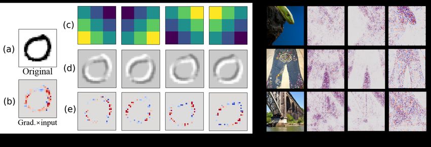
Figure 6: (a) The interpretation of an entire ’green mamba’ class. The color filter scores and edge
filter scores are shown. (b) An example of the ’steel arch bridge’ class. The original image and its
color filter scores are on the left side. The red and blue channels of the original image are shown in
the center. The magnitude of each color channel is shown with colors. The sky background is not
considered for classification as indicated in the color filter score.
the orientations of green mambas are various since there are no particular patterns. At the same
time, Figure 6 (b) indicates how the NN removes the background from the image to classify it. The
sky in the image has a high magnitude in the blue channel. To get rid of the background, the NN
subtracts the blue channel from the red channel as shown in the color filter scores. Thus, the NN
uses the color difference to distinguish the background and the target objects. The blue filter score
in Figure 6 (a) also suggests that the NN generally uses the blue color to locate the green mamba in
the image by eliminating the background since the bright colors have high magnitudes in all color
channels. For example, the first row on the right side of Figure 1 shows a green mamba in the blue
background. The filter score image with respects to the input pixels indicates that the NN spots the
green mamba successfully by subtracting blue colors from the red channel.
The edge filter scores indicate important edges in the image. If the target object is horizontally
located, south and north filters become important in the image. Furthermore, if there are several
edges with various objects in the image, then the edges of the target objects are chosen as the most
important contributors. For example, when a tree branch and a green mamba are in the same image,
the NN separates them by utilizing different color edge filters.
The pixel-wise interpretation of GF-ResNet’s filter score images performs better than the saliency
map and the gradient×input as shown in Figure 1. Our model successfully selects the regions of the
target object in the image even when other methods fail. We think that the interpretable components
of the GF-ResNet force the NN to select filter-created features, i.e. different edges in the image so
that the interpretability and the accuracy are improved.
5 C ONCLUSION
In this paper, we successfully implemented predefined and commonly used image kernels into CNNs
and ResNet-50, named as GFNN and GF-ResNet. Our models were trained with MNIST, and Im-
ageNet datasets and produced impressive performances for large-scale object recognition tasks (up
to 92.1% top-5 and 74.6% top-1 on ImageNet). Filter scores and filter score images defined in 2.1.3
are useful metrics for quantifying relative importances of each predefined kernels. We showed how
DNNs utilize image kernels to classify digits and images according to their shapes and colors with
various datasets.
8Under review as a conference paper at ICLR 2020
R EFERENCES
Sebastian Bach, Alexander Binder, Grégoire Montavon, Frederick Klauschen, Klaus Robert Müller,
and Wojciech Samek. On pixel-wise explanations for non-linear classifier decisions by layer-wise
relevance propagation. PLoS ONE, 10(7):1–46, 2015.
Wieland Brendel and Matthias Bethge. Approximating CNNs with bag-of-local-features models
works surprisingly well on imagenet. In International Conference on Learning Representations
(ICLR), 2019.
Kaiming He, Xiangyu Zhang, Shaoqing Ren, and Jian Sun. Deep residual learning for image recog-
nition. In The IEEE Conference on Computer Vision and Pattern Recognition (CVPR), 2016.
Jay Hoon Jung, Yousun Shin, and YoungMin Kwon. A metric to measure contribution of nodes in
neural networks. In IEEE Symposium Series on Computational Intelligence (SSCI), 2019.
Alex Krizhevsky, Ilya Sutskever, and Geoffrey E Hinton. Imagenet classification with deep convo-
lutional neural networks. In Advances in Neural Information Processing Systems (NIPS), 2019.
Zheng Liang, Yang Yi, and Tian Qi. Sift meets cnn: A decade survey of instance retrieval. IEEE
Transactions on Pattern Analysis and Machine Intelligence, 2016.
Gueguen Lionel, Sergeev Alex, Kadlec Ben, Liu Rosanne, and Yosinski Jason. Faster neural net-
works straight from jpeg. In Advances in Neural Information Processing Systems (NIPS). 2018.
Avanti Shrikumar, Peyton Greenside, Anna Shcherbina, and Anshul Kundaje. Not Just a Black Box:
Learning Important Features Through Propagating Activation Differences. 2016.
Karen Simonyan, Andrea Vedaldi, and Andrew Zisserman. Deep inside convolutional networks: Vi-
sualising image classification models and saliency maps. In International Conference on Learning
Representations, (ICLR), 2014.
Tianjun Xiao, Yichong Xu, Kuiyuan Yang, Jiaxing Zhang, Yuxin Peng, and Zheng Zhang. The
application of two-level attention models in deep convolutional neural network for fine-grained
image classification. In IEEE Conference on Computer Vision and Pattern Recognition (CVPR),
2015.
9Under review as a conference paper at ICLR 2020
A A PPENDIX
A.1 L IST OF I MAGE P ROCESSING K ERNELS .
A.1.1 S HARPENING
0 −1 0 −1 −1 −1 1 −2 1
! ! !
−1 5 −1 −1 9 −1 −2 5 −2
0 −1 0 −1 −1 −1 1 −2 1
A.1.2 E MBOSSING
1 0 0
!
0 0 0
0 0 −1
A.1.3 B LURRING
1/9 1/9 1/9 1/16 1/8 1/16
! !
1/9 1/9 1/9 1/8 1/4 1/8
1/9 1/9 1/9 1/16 1/8 1/16
A.1.4 E DGE : E AST
1 1 −1 5 −3 −3 1 0 −1 1 0 −1
! ! ! !
1 −2 −1 5 0 −3 1 0 −1 2 0 −2
1 1 −1 5 −3 −3 1 0 −1 1 0 −1
A.1.5 E DGE : N ORTHEAST
1 −1 −1 −3 −3 −3 0 −1 −1 0 −1 −2
! ! ! !
1 −2 −1 5 0 −3 1 0 −1 1 0 −1
1 1 1 5 5 −3 1 1 0 2 1 0
A.1.6 E DGE : N ORTH
−1 −1 −1 −3 −3 −3 −1 −1 −1 −1 −2 −1
! ! ! !
1 −2 1 −3 0 −3 0 0 0 −1 0 1
1 1 1 5 5 5 1 1 1 0 1 2
A.1.7 E DGE : N ORTHWEST
−1 −1 1 −3 −3 −3 1 −1 0 −2 −1 0
! ! ! !
1 −2 1 −3 0 5 −1 0 1 −1 0 1
1 1 1 −3 5 5 0 1 1 0 1 2
A.1.8 E DGE : W EST
−1 1 1 −3 −3 5 −1 0 1 −1 0 1
! ! ! !
−1 −2 1 −3 0 5 −1 0 1 −2 0 2
−1 1 1 −3 −3 5 −1 0 1 −1 0 1
A.1.9 E DGE : S OUTHWEST
1 1 1 −3 5 5 0 1 −1 0 1 2
! ! ! !
−1 −2 1 −3 0 5 −1 0 1 −1 0 1
−1 −1 1 −3 −3 −3 −1 −1 0 −2 −1 0
A.1.10 E DGE : S OUTH
1 1 1 5 5 5 1 1 1 1 2 1
! ! ! !
1 −2 1 −3 0 −3 0 0 0 0 0 0
−1 −1 −1 −3 −3 −3 −1 −1 −1 −1 −2 −1
10Under review as a conference paper at ICLR 2020
A.1.11 E DGE : S OUTHEAST
1 1 1 5 5 −3 1 1 0 2 1 0
! ! ! !
1 −2 −1 5 0 −3 1 0 −1 1 0 −1
1 −1 −1 −3 −3 −3 0 −1 −1 0 −1 −2
A.1.12 E DGE : S ECOND O RDER D ERIVATIVE O PERATEORS
0 −1 0 −1 −1 −1
! !
−1 4 −1 −1 8 −1
0 −1 0 −1 −1 −1
A.1.13 F IRST O RDER D ERIVATIVE
0 0 −1 −1 0 0 1 0 −1 −1 −1 −1
! ! ! !
0 1 0 0 1 0 1 0 −1 0 0 0
0 0 0 0 0 0 1 0 −1 1 1 1
√
1 0 −1 −1 −2 −1 √1 0 −1 −1 − 2 −1
! !
√
2 0 −2 0 0 0 2 0 − 2 0
√0 0
1 0 −1 1 2 1 1 0 −1 1 2 1
11You can also read