The Economic Implications of Climate-Induced Changes in Agricultural Production - Report to NIWA - Motu ...
←
→
Page content transcription
If your browser does not render page correctly, please read the page content below
The Economic Implications
of Climate-Induced Changes
 in Agricultural Production

        Report to NIWA

    Prepared by Infometrics Ltd

           August 2011
CONTENTS
1. Summary .......................................................... 1
2. Climate Scenarios............................................... 2
3. Economic Modelling ............................................ 5
BAU Scenario ................................................................................ 5
Climate Scenarios .......................................................................... 5
4. Model Results .................................................... 7
BAU Scenario ................................................................................ 7
Climate Scenarios .......................................................................... 8
Comparison with Other Research ................................................... 12
Appendix A: The ESSAM Model .................................. 15
Appendix B: The BAU Scenarios ................................ 19
2030/31 ..................................................................................... 19
2060/61 and 2090/91 .................................................................. 20
Authorship
This report has been prepared by Dr Adolf Stroombergen.
Email: astro@infometrics.co.nz
All work and services rendered are at the request of, and for the purposes of the
client only. Neither Infometrics nor any of its employees accepts any responsibility
on any grounds whatsoever, including negligence, to any other person or
organisation. While every effort is made by Infometrics to ensure that the
information, opinions and forecasts are accurate and reliable, Infometrics shall not
be liable for any adverse consequences of the client’s decisions made in reliance of
any report provided by Infometrics, nor shall Infometrics be held to have given or
implied any warranty as to whether any report provided by Infometrics will assist
in the performance of the client’s functions1. SUMMARY
Two previous papers, Tait et al (2005) and Infometrics (2008) 1, looked at the
effects of climate on agricultural production by econometrically estimating the
effect of climate variability (in particular, drought) on the production of milksolids
and meat with a panel dataset, and then incorporating the production effects into
a general equilibrium model in order to assess the economy-wide implications of
changes in agricultural production.
The results showed negative economic effects. A reduction in sheep and beef
output of 5% together with a reduction in dairy output of about 10% (based on
the estimated effects of the 1998/99 drought) led to a reduction in private
consumption of around 0.7% and a reduction in gross domestic product of over
1%. Greenhouse gas emissions declined by more than 5%.
In this paper we again analyse the effects of climate-induced changes in
agricultural production, and include forestry as well. We pursue a different
methodology to estimate the effects of future climate change on agricultural and
forestry output. Instead of looking at adverse climatic events, notably droughts,
this study is focussed on the longer term impacts of projected climate change
based on a number of models and scenarios. There is also explicit modelling of
the relationship between temperature, water availability and plant growth. As
before the results are then fed into a general equilibrium model of the New
Zealand economy.
Some of the climate change scenarios indicate more drought-like conditions,
mainly for eastern regions, while others indicate little change. In addition, other
regions such as Southland experience wetter and warmer conditions.
Under some scenarios the wider economic effects are negative, but most results
show a positive effect. Changes in real gross national disposable income range
from -0.2% to 1.8% and changes in gross domestic product vary between -0.4%
and 3.9% – all relative to a situation of no climate change. Changes in
agricultural and forestry output are an order of magnitude larger, with
Horticultural output showing the most sensitivity to climate change.
The difference in direction between the earlier results and those obtained in this
paper are largely because plants, animals and farm management are adversely
affected by short term departures from ‘normal’ climatic conditions, whereas
progressive climate change over many decades allows more time for adaptation –
albeit not unlimited.
1
Stroombergen (2008): The Economic Implications of Climate-Induced Variations in Agricultural
Production. Infometrics report to NIWA, May.
Tait A.B.; Renwick, J.A. and Stroombergen, A.H. (2005): The economic implications of climate-induced
variations in milk production. NZ Journal of Agricultural Research, 48, 213–225.
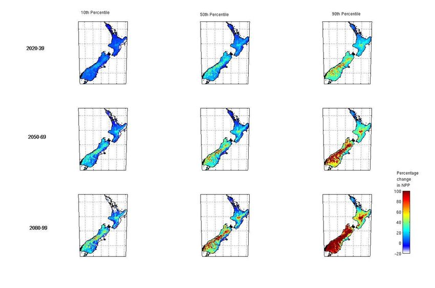
12. CLIMATE SCENARIOS
The effects of climate change on agriculture were estimated by NIWA by
calculating each region’s net photosynthesis using a model of the relationship
between water availability and growth, as well as the regulation of growth by
temperature.
Climate changes over three future periods were examined; 2020-39 (midpoint
reference year 2030), 2050-69 (2060) and 2080-99 (2090), using information
from three emissions scenarios and 19 global climate models. The period 1980-
99 (1990) was chosen as the baseline climate. This produced a wide range of
results for each time period, as summarised in Table 1 below by the changes in
Net Primary Production (NPP) at the 10th percentile, median and 90th percentile.
Figure 1 shows the geographical spread of these changes.
Industry aggregation is based on 2007 land use data derived from the agri-quality
data set.
Table 1: Projected Changes in Net Primary Production
All Arable Dairy Horticulture Forestry Sheep/beef
Percentage change in NPP: 2030-49 from 1980-99
Low-10th Percentile -1.45 -1.09 -1.78 -1.72 -0.66 -1.46
Median 9.17 7.78 9.24 9.53 9.29 9.04
High-90th Percentile 25.47 18.42 25.39 23.98 26.61 26.96
Percentage change in NPP: 2050-69 from 1980-99
Low-10th Percentile -4.93 -1.21 -5.36 -5.52 -3.13 -4.19
Median 15.57 13.93 15.84 14.83 16.23 15.31
High-90th Percentile 46.39 38.93 45.50 44.35 49.17 49.65
Percentage change in NPP: 2080-99 from 1980-99
Low-10th Percentile -12.30 -3.70 -13.18 -8.15 -10.39 -12.74
Median 20.21 18.66 20.82 19.40 20.75 19.43
High-90th Percentile 75.04 51.86 73.96 71.86 78.75 85.08
The results reveal an interesting picture:
1. The changes in NPP cover a range from modest decreases to large
increases, and appear to become more pronounced with time at different
ends of the range.
2. As expected there is not a great deal of difference between industries
given the integrated land use in New Zealand (high within region
elasticity).
23. However, the detailed results show more variability, manifested as
extensions to the autumn and spring growing seasons and much deeper
summer droughts. Thus the aggregated results used to estimate the
economic effect of climate change do not necessarily reflect risk at any
given farm gate.
4. In some regions the thermal environment for plant production remains
largely within the optimal range, so large changes in terms of the pasture
experiencing below wilting point conditions are infrequent. Other regions
see changes beyond the wilting point threshold.
5. The usual east coast/Northland drying effect is evident, even as early as
2030 for the low scenario. There is a large range in responses across the
North Island driven by inter-model rainfall variability. We also see
conditions becoming too hot for growth later on in the century to the
north, but enhancing it in the south.
6. Adaptation is not modelled. For example dairying might shift out of
Northland, kiwifruit might move from the Bay of Plenty to Nelson, high
sugar c4 grasses might be developed for the northern Waikato, and of
course irrigation could be expanded in some eastern regions, although this
may not always be cost-effective
7. The dominant signal if we look at the median results, is for an overall
increase in New Zealand NPP over time, which stems from large increases
in NPP in West Coast, Southland, Otago and central North Island regions,
offset somewhat by smaller decreases or no change in Canterbury, and
eastern and northern North Island.
8. The message from the range of results is that while reduced or no change
in NPP for much of New Zealand is possible, there is also a
significant probability of little change to substantial increases in NPP for
much of the country.
3Figure 1: Projected Changes in Net Primary Production 4
3.         ECONOMIC MODELLING
    BAU Scenario
Business as Usual (BAU) scenarios are developed which represent pictures of the
economy at three snapshot points in the future, in this case 2030/31, 2060/61
and 2090/91, as representative of the periods 2020-39, 2050-69 and 2080-99
respectively.

The BAUs are not necessarily the most likely forecasts of what the economy might
look like. Indeed it is impossible to predict how the economy might evolve over
such distant horizons. Rather the BAUs are intended to be plausible projections
of the economy that can constitute a frame of reference against which other
scenarios may be compared. The BAUs do not take into account any effects of
climate change – not domestically nor internationally, although they do include
carbon prices.

It also assumed that over time New Zealand takes on progressively tighter
obligations of responsibility for emissions. Any excess needs to be covered by
purchasing emission permits on the international market. Carbon prices are
assumed to increase over time and New Zealand’s Emissions Trading Scheme
(ETS) is integrated into the world market.

                 Table 2: BAU Emission Obligations and Prices

                                                    2030/31     2060/61    2090/91
   Responsibility target as % of 1990 emissions      85%         50%        20%
   Carbon price (real $NZ/tonne CO2e)                $100        $150       $200

For 2030/31 it is assumed that the free allocation of New Zealand emission units
will be as currently legislated under the ETS. However, for 2060/61 and 2090/91
we assume no free allocation. For all years no explicit allowance is made for net
forestry emissions, as these are as likely to be positive as negative. In any case
any credit or debit in this regard does not significantly alter the relative effects of
climate change.

Further detail on the BAUs is given in Appendix B.

Given the BAUs the model is then ‘shocked’ with a number of scenarios, described
in the following section.

    Climate Scenarios
The following nine climate change scenarios are examined, treating the changes
in NPP in Table 1 as changes in productivity relative to BAU. That is, gross output
in the four agricultural industries and in the forestry industry can change by the
amounts in Table 1 without any changes in inputs of land, labour or capital. In no
scenario is the model forced to increase or reduce output. The output response is
endogenous, depending on the specified productivity shock, the price and scarcity
of resources, the ability to sell more output in local and foreign markets, and so
on.

                                                                                      5
Table 3 Scenario Specification
2030/31 2060/61 2090/91
Low-10th Percentile 31L 61L 90L
Median 31M 61M 91M
High-90th Percentile 31H 61H 91H
For all scenarios a number of macroeconomic closure rules are adopted.
1. Capital market closure: Rates of return on capital are held constant at BAU
levels, with capital formation being the equilibrating variable.
2. Labour market closure: Total employment is held constant at the BAU
level, with wage rates being the endogenous equilibrating mechanism.
While employment may be more variable than wage rates in the short run,
in the medium term the nature of the labour market in New Zealand means
that how the economy adjusts to climate change is more likely to affect
wage rates than employment.
3. External closure: The balance of payments is a fixed proportion of nominal
GDP, with the real exchange rate being endogenous. This means that any
adverse shocks are not met simply by borrowing more from offshore, which
is not sustainable in the long term.
4. Fiscal closure: The fiscal surplus is held constant at the BAU level, with
personal income tax rates being endogenous.
64. MODEL RESULTS
BAU Scenario
Although we do not wish to place any emphasis on the BAU scenarios, especially
the more distant ones, it may be useful to sketch a rough picture of what the
economy might look like at least for 2030/31. Table 4 summarises the results.
Table 4: Business as Usual Scenario to 2030/31
% pa % pa
2006- 2001-
2031 2011
Private Consumption 2.1 2.9
Investment 2.0 3.9
Exports 2.8 2.6
Imports 2.2 4.3
GDP 2.2 2.6
RGNDI 2.3 2.9
Population 0.8 1.3
RGNDI/capita 1.5 1.6
CO2e 0.5 0.8
CO2e/capita -0.3 -0.5
Excess emissions (Mt) 31.5 NA
* December years 2001 and 2010
In spite of the global financial crisis from 2007, the decade to 2001-2011 saw
reasonable economic growth with Gross Domestic Product (GDP) rising at an
average annual rate of 2.6% and Real Gross National Disposable Income (RGNDI)
at 2.9% pa.2 Population expansion meant that RGNDI per capita rose rather less
quickly at 1.6% pa, but this is still marginally stronger than what is envisaged
over the period to 2030/31. Projected growth is slower for a number of reasons:
Lingering effects of the global financial crisis, both in New Zealand and
overseas, the latter having a direct effect on New Zealand’s exports.
An aging labour force.
An obligation to purchase emission permits on world markets to cover
excess emissions (see previous section).
Higher oil prices, and New Zealand still a net importer of oil based fuels.
The projected increase in CO2 emissions is only 0.5% pa compared to 0.8% pa
over the last decade. Slower population and economic growth contribute to this
result. On a per capita basis the negative growth is attributable to emissions
pricing and increases in energy efficiency, whereas the historical decline in per
2
RGNDI is equivalent to GDP with adjustments for changes in the terms of trade and net remittances
overseas.
7capita emission is largely attributable to more electricity generation from
renewables.
Climate Scenarios
Table 6 summarises the macroeconomic results and the changes in gross output
in the agricultural and forestry industries for each of the future scenarios.
With the magnitude of the climate shocks rising over time, positively and
negatively, it is not surprising to see that the changes in GDP also increase over
time, reaching a maximum of 3.9% in Scenario 91H.
The component of final demand that shows the largest increase is exports. In
fact the changes in exports are about twice as large, proportionately, as the
changes in GDP. Given the weight of agricultural products in New Zealand’s
exports, and the magnitude of the exogenous changes in NPP, this is not
surprising.
However, not all of the changes in NPP are translated into more exports. Exports
are not an end in themselves – they are the means to buy imports which are
essential to raising economic welfare. A more favourable growing climate (or
analogously a productivity enhancing technological development) means that
fewer resources such as labour and capital are required to maintain a given level
of agricultural exports. In fact agricultural output expands and uses fewer
resources, allowing them to be allocated to the production of other consumer
goods and services.
Hence private consumption also rises, with household demand being met by both
more domestic production and more imports, the latter paid for by the lift in
export receipts.
The changes in RGNDI are always less (absolutely) than the changes in GDP.
This occurs for two main reasons:
1. Whenever agricultural productivity rises, output from those industries
expands, leading to higher GHG emissions. As shown in Figure 2 the
relationship between the change in agricultural output and the change in
CH4 and N2O emissions is almost linear. The extra emissions have to be
offset by purchasing emissions permits on the world market, meaning that
some of the increase in national income goes offshore.
Taking Scenario 31H as an example, the increase in emissions relative to
BAU of 3.3% is about 2800 MT. At a carbon price of $100/tonne the cost
of emission permits is about 0.1% of GDP. This effect increases over time
in line with the rising carbon price, reaching 0.5% of GDP in Scenario 91H
when the much higher NPP causes total GHG emissions to rise by almost
11%, and CH4 and N2O emissions by over 16%.
2. The larger effect though is from changes in the terms of trade. As
agricultural production expands producers are forced down the demand
curve in order to sell the extra output. Again taking Scenario 31H as an
example, if there was no change in the terms of trade the change in
RGNDI would be 1.2%, only just under the change in GDP. Effectively
some of the benefits of higher agricultural (and forestry) productivity are
transferred to foreign customers.
8Figure 2: Changes Agricultural Output and non-CO2 Emissions
Primary exporters, especially co-operatives, tend to be production-driven. Any
new technology or favourable change in the climate that lowers the cost of
production may generate some short-term super-normal profits, but supply rises
eventually as existing farmers increase production and new entrants move into
the industry. Unless the co-operative is a very small player in the market into
which it sells, that increase in supply will force the co-operative to look at offering
price reductions or to search for lower value markets.
In Scenario 91H, the most optimistic of the nine examined, the increase in the
volume of exports of dairy, meat, wool, horticultural products and logs is about
47%, so a reduction in the terms of trade of just under 5% is not implausible.
A new equilibrium is established, characterised by greater output and lower prices
than existed before the climate-induced productivity boost. The rate of return will
be as it was before, with the positive productivity effect offset by some
combination of higher input costs, such as for land, and lower product prices. The
relative sizes of these two effects are determined by the price elasticities of
demand for output and factor substitution possibilities.
The reduction in product prices is of course beneficial to consumers, but that
converts into a gain in national economic welfare (RGNDI) only if those
consumers live in New Zealand. As most of New Zealand’s agricultural output is
exported, it is foreign consumers who capture a large part of the benefit of on-
farm NPP improvements. This is manifested as a decline in the terms of trade,
which is evident in Table 6. Of course foreign consumers also share in the losses
when NPP declines.
At the industry level, the agricultural sub-industry that is most sensitive to the
NPP shocks is Horticulture. See Figure 3. It probably has less scope to adapt to
adverse climatic shocks compared to other types of farming. Equally, under
favourable climate changes production can increase without requiring much in the
way of other inputs.
9Figure 3: Changes in NPP and Agricultural Output
As shown in Figure 4 the change in agricultural production tends to be about half
of the change in NPP, suggesting a combination of offsets due to higher input
prices and some transfer of the positive income effects of increases in productivity
spilling over to other industries. That is, because the price elasticity of demand
for food is less than one, a given percentage reduction in its price is not met with
a corresponding increase in demand. Some of the gain that consumers receive is
instead used to buy more goods and services that have a higher income elasticity
of demand. This mechanism is just the demand side of the reallocation of
resources on the supply side from exporting to consumption, discussed above.
Figure 4: Changes in NPP and Agricultural Output
After Horticulture, Forestry shows the next largest changes in output (Figure 3),
though it does also experience some of the largest NPP shocks. Log exports are
more of a ‘commodity’ than most agricultural exports and New Zealand is a small
player in the world market compared to its position in the market for goods such
10as milk powder, coarse wools and gold kiwifruit. Hence an increase in New
Zealand production would have an imperceptible effect on world prices.
Nevertheless as forestry pushes into more marginal land (even in the presence of
favourable climate shocks) we might expect to see lower value logs being
produced. So even if the price of any particular grade of log does not fall as
supply from New Zealand rises, the average price received for a basket of New
Zealand logs may decline somewhat.
Sensitivity Test
In this scenario we re-run Scenario 91H with doubled export relative price
elasticities of demand for the four agricultural commodities and logs, from the
default values shown in Table 5. This is labelled Scenario 91Ha in Table 6.
Table 5: Export Relative Price Elasticities of Demand
Commodity PED
Dairy and Meat 1.2
Horticulture 3.5
Logs 4.0
The higher elasticities are not intended to be of equal merit to the standard
elasticities. Those for horticulture and logs are already quite high and so doubling
them could lead to some unrealistic changes in output. In the case of horticulture
for example the doubled elasticity means that a 10% increase in the price of
horticultural products from New Zealand relative to the price of horticultural
products from other countries would lead to a 70% drop in the quantity
demanded.
As we are interested in knowing how the effects of a climate shock differ if some
behavioural parameters (in this case export elasticities) are different, the BAU
also has to be re-run with the doubled elasticities. If this is not done a
comparison of Scenario 91Ha with the original BAU would confound the effects of
climate change with the effects of changing the elasticities. It would be as if
climate change caused the elasticities to be different.
The increase in GDP in Scenario 9Ha is 6.2% compared to 3.9% in Scenario 9H,
and the corresponding figures for RGNDI are 3.8% and 1.8%. Total emissions
rise by 18.0% in Scenario 9Ha compared to 10.8% in Scenario 9H, with figures
for agricultural non-CO2 emissions of 28.7% and 16.1% respectively.
As expected there are some dramatic increases in primary output with the
Forestry harvest nearly doubling and Horticulture output surging by over 200%.
Although 2090 is a distant horizon, a change of 200% still implies an extra 1.4%
per annum growth over BAU in every year. Whether these sorts of increases can
occur without ever more marginal land having to be used at escalating unit cost
(and perhaps with undesirable environmental effects as well) is a moot point, but
the implication is that the results in Scenario 9Ha are probably over-optimistic.
Perhaps the key message to take from these results is that the more price
sensitive foreign consumers are, the greater the potential gain to New Zealand
from favourable climate change that lowers agricultural production costs,
provided the increase in foreign demand can be met without generating higher
domestic costs (including environmental costs) that offset the favourable effect of
the productivity enhancement. The alternative scenario is that our export mix is
focused less on commodities implying less reliance on a pure quantity response as
11the means by which the country benefits from favourable climate change. It
would also mean greater resilience to adverse climate change, which is within the
probability distributions for net primary production estimated by NIWA.
Comparison with Other Research
Tait et al (2005) and Infometrics (2008)3, looked at the effects of climate change
on agricultural production by econometrically estimating the effect of climate
variability on the production of milksolids and meat, using a combined cross-
section (by region) time series approach. The production effects were then
incorporated into a general equilibrium model in order to assess the economy-
wide implications of changes in agricultural productivity induced by climate
change.
In terms of the size of effects, a change of one standard deviation in Days of Soil
Moisture Deficit (DSMD) was estimated to lead to a 3-4% change in milksolids
production per cow. With respect to meat, an increase of one standard deviation
in DSMD was estimated to reduce the average slaughter weight of cattle by 2-3%
and the average slaughter weight of sheep by about 4-7%. While these effects
are statistically significant, in the case of beef they are generally smaller than the
differences between regions, and in the case of sheep meat they correspond to
about four years worth of ongoing productivity improvement at historical rates.
Modelling results showed that a reduction in sheep and beef output of 5%
together with a reduction in dairy output of about 10% (based on the estimated
effects of the 1998/99 drought) leads to a reduction in private consumption of
around 0.7% and a reduction in GDP of over 1%. Greenhouse gas emissions
decline by more than 5%.
While the new results confirm that the effects of climate change can be negative,
positive effects predominate over the next century or so.
The main reason for this apparent inconsistency is that fundamentally different
things are being examined. The earlier work captured the effects of temporary
departures from normal climatic conditions – short term variability such as
drought – while in this report we look at effects of persistent longer term climate
change. Presumably plants and animals are better able to adapt to the latter. Of
course departures from normal climatic conditions will still occur in a future where
‘normal’ could be climatically more favourable than in the past.
The previous econometric work dealt directly with changes in the physical amount
of agricultural output – notably milksolids and meat, not with changes in Net
Primary Production. While over the longer term we would expect changes in NPP
to be a reasonable proxy for changes in any kind of farming output, adaption to
seasonal variation with regard to water availability for example, or changes in
animal physiology, could lead to divergences between NPP and animal output over
the next few decades. This might mean that the NPP-based results are over-
optimistic.
3
Op cit
12Finally, a forthcoming paper by Reisinger and Stroombergen 4 uses two global
models to look at the effects of climate change mitigation on world agricultural
output and world agricultural commodity prices (albeit that the focus of the paper
is on alternative GHG exchange rate metrics). An important finding is that
worldwide the effects of climate change mitigation are expected to lead to higher
agricultural prices, thus providing a counteracting force to the downward pressure
in New Zealand caused by favourable climate change. If this is correct the
implication is that New Zealand will enjoy even larger economic benefits from
longer term climate change than those estimated above.
The final piece in the jigsaw is to understand the direct effect of climate change
on world agricultural production, along the lines of exploratory research in
Stroombergen (2009).5 To further progress that research means addressing
possible differences between the effects of climate change on New Zealand’s
agricultural output estimated by global models versus those estimated by NIWA –
as above. The latter should be more accurate as in global models New Zealand is
typically combined with other countries in the Asia Pacific region. Regardless of
which projections are better, however, an inconsistency could arise with regard to
world agricultural commodity prices as for some commodity prices the actions of
New Zealand are not totally irrelevant.
4
Reisinger, A and Stroombergen, A. (2011): Implications of alternative metrics to account for non-CO2 GHG
emissions. Report prepared for Ministry of Agriculture and Forestry.
5
Stroombergen (2009): The International Effects of Climate Change on Agricultural Commodity Prices,
and the Wider Effects on New Zealand. Infometrics report to Motu.
13Table 6: Summary of Results of Climate Change Scenarios
Scenario 31L 31M 31H 61L 61M 61H 91L 91M 91H 91Ha
2030/31 2060/61 2090/91
Low Median High Low Median High Low Median High High
AAU (MT) 52.2 52.2 52.2 30.7 30.7 30.7 12.3 12.3 12.3 12.3
CO2 price ($/tonne) $100 $100 $100 $150 $150 $150 $200 $200 $200 $200
% ∆ on BAU
Private Consumption 0.0 0.3 0.9 -0.1 0.5 1.6 -0.2 0.5 2.1 4.7
Exports -0.1 1.0 2.9 -0.4 1.6 5.8 -0.9 1.9 10.0 16.1
Imports 0.0 0.3 1.0 -0.2 0.6 2.3 -0.3 0.7 3.5 8.7
GDP -0.1 0.5 1.3 -0.2 0.7 2.4 -0.4 0.8 3.9 6.2
RGNDI 0.0 0.3 0.7 -0.1 0.4 1.3 -0.2 0.4 1.8 3.8
Terms of Trade 0.1 -0.6 -1.6 0.2 -0.8 -2.9 0.5 -1.0 -4.9 -4.9
CO2e -0.2 1.1 3.3 -0.6 2.1 7.1 -1.2 2.3 10.8 18.0
CH4 & N2O -0.3 1.7 5.0 -1.0 3.3 11.1 -1.8 3.5 16.1 28.7
Gross Output
Horticulture -1.2 7.3 20.8 -4.5 14.3 54.4 -6.0 16.0 87.9 219.1
Livestock and cropping -0.3 1.8 5.2 -1.1 4.0 13.8 -2.1 4.1 20.2 35.4
Dairy cattle farming -0.3 1.6 4.5 -0.8 2.5 7.8 -1.5 2.6 10.9 17.2
Other farming -0.4 2.4 6.8 -1.4 6.1 21.3 -2.5 6.6 30.9 62.1
Forestry -0.3 3.7 11.9 -1.4 8.3 31.7 -3.9 9.2 50.5 94.2
14APPENDIX A: THE ESSAM MODEL
The ESSAM (Energy Substitution, Social Accounting Matrix) model is a general
equilibrium model of the New Zealand economy. It takes into account the main
inter-dependencies in the economy, such as flows of goods from one industry to
another, plus the passing on of higher costs in one industry into prices and thence
the costs of other industries.
The ESSAM model has previously been used to analyse the economy-wide and
industry specific effects of a wide range of issues. For example:
Energy pricing scenarios
Changes in import tariffs
Faster technological progress
Policies to reduce carbon dioxide emissions
Funding regimes for roading
Some of the model’s features are:
53 industry groups, as detailed in the table below.
Substitution between inputs into production - labour, capital, materials,
energy.
for energy types: coal, oil, gas and electricity, between which substitution
is also allowed.
Substitution between goods and services used by households.
Social accounting matrix (SAM) for complete tracking of financial flows
between households, government, business and the rest of the world.
The model’s output is extremely comprehensive, covering the standard collection
of macroeconomic and industry variables:
GDP, private consumption, exports and imports, employment, etc.
Demand for goods and services by industry, government, households and
the rest of the world.
Industry data on output, employment, exports etc.
Import-domestic shares.
Fiscal effects.
Production Functions
These equations determine how much output can be produced with given
amounts inputs. A two-level standard translog specification is used which
distinguishes four factors of production – capital, labour, and materials and
energy; with energy split into coal, oil, natural gas and electricity. Land is also
included for agriculture and forestry
Intermediate Demand
A composite commodity is defined which is made up of imperfectly substitutable
domestic and imported components - where relevant. The share of each of these
components is determined by the elasticity of substitution between them and by
relative prices.
15Price Determination The price of industry output is determined by the cost of factor inputs (labour and capital), domestic and imported intermediate inputs, and indirect tax payments. World prices are not affected by New Zealand purchases or sales abroad. Consumption Expenditure This is divided into Government Consumption and Private Consumption. For the latter eight household commodity categories are identified, and spending on these is modelled using price and income elasticities in an AIDS framework. An industry by commodity conversion matrix translates the demand for commodities into industry output requirements and also allows import-domestic substitution. Government Consumption is usually either a fixed proportion of GDP or is set exogenously. Where the budget balance is exogenous, either tax rates or transfer payments are assumed to be endogenous. Stocks Owing to a lack of information on stock change, this is exogenously set as a proportion of GDP, domestic absorption or some similar macroeconomic aggregate. The industry composition of stock change is set at the base year mix, although variation is permitted in the import-domestic composition. Investment Industry investment is related to the rate of capital accumulation over the model’s projection period as revealed by demand for capital in the horizon year. Allowance is made for depreciation. Rental rates or the service price of capital (analogous to wage rates for labour) also affect capital formation. Investment by industry of demand is converted into investment by industry of supply using a capital input- output table. Again, import-domestic substitution is possible between sources of supply. Exports Exports are determined from overseas export demand functions in relation to world prices and domestic prices inclusive of possible export subsidies, adjusted by the exchange rate. Export quantities can also be set exogenously. Supply-Demand Identities Supply-demand balances are required to clear all product markets. Domestic output must equate to the demand stemming from consumption, investment, stocks, exports and intermediate requirements. Balance of Payments Receipts from exports plus net capital inflows (or borrowing) must be equal to payments for imports; each item being measured in domestic currency net of subsidies or tariffs. 16
Factor Market Balance

In cases where total employment of a factor is exogenous, factor price relativities
(for wages and rental rates) are usually fixed so that all factor prices adjust equi-
proportionally to achieve the set target.

Income-Expenditure Identity

Total expenditure on domestically consumed final demand must be equal to the
income generated by labour, capital, taxation, tariffs, and net capital inflows.
Similarly, income and expenditure flows must balance between the five sectors
identified in the model – business, household, government, foreign and capital.

Industry Classification

The 53 industries identified in the ESSAM model are defined below. Industries
definitions are according to Australian and New Zealand Standard Industrial
Classification (ANZSIC). For the five agricultural industries in the model the finer
definitions are as follows.

             A011100   Plant Nurseries                               1
             A011200   Cut Flower and Flower Seed Growing            1
             A011300   Vegetable Growing                             1
             A011400   Grape Growing                                 1
             A011500   Apple and Pear Growing                        1
             A011600   Stone Fruit Growing                           1
             A011700   Kiwi Fruit Growing                            1
             A011910   Citrus Growing                                1
             A011920   Berry Fruit Growing                           1
             A011990   Other Fruit Growing nec                       1
             A012100   Grain Growing                                 2
             A012200   Grain-Sheep and Grain-Beef Cattle Farming     2
             A012300   Sheep-Beef Cattle Farming                     2
             A012400   Sheep Farming                                 2
             A012500   Beef Cattle Farming                           2
             A013000   Dairy Cattle Farming                          3
             A014100   Poultry Farming (Meat)                        4
             A014200   Poultry Farming (Eggs)                        4
             A015100   Pig Farming                                   4
             A015200   Horse Farming                                 4
             A015300   Deer Farming                                  4
             A015910   Mixed Livestock                               2
             A015930   Beekeeping                                    4
             A015990   Livestock Farming nec                         4
             A016910   Tobacco and Hops Growing                      4
             A016920   Cultivated Mushroom Growing                   4
             A016990   Crop and Plant Growing nec                    4
             A021200   Shearing Services                             5
             A021300   Aerial Agricultural Services                  5
             A021900   Services to Agriculture nec                   5
             A022000   Hunting and Trapping                          5

                                                                                   17
1 HFRG Horticulture and fruit growing
2 SBLC Livestock and cropping farming
3 DAIF Dairy and cattle farming
4 OTHF Other farming
5 SAHF Services to agriculture, hunting and trapping
6 FOLO Forestry and logging
7 FISH Fishing
8 COAL Coal mining
9 OIGA Oil and gas extraction, production & distribution
10 OMIN Other Mining and quarrying
11 MEAT Meat manufacturing
12 DAIR Dairy manufacturing
13 OFOD Other food manufacturing
14 BEVT Beverage, malt and tobacco manufacturing
15 TCFL Textiles and apparel manufacturing
16 WOOD Wood product manufacturing
17 PAPR Paper and paper product manufacturing
18 PPRM Printing, publishing and recorded media
19 PETR Petroleum refining, product manufacturing
20 CHEM Fertiliser and other industrial chemical manufacturing
21 RBPL Rubber, plastic and other chemical product manufacturing
22 NMMP Non-metallic mineral product manufacturing
23 BASM Basic metal manufacturing
24 FABM Structural, sheet and fabricated metal product manufacturing
25 MAEQ Machinery and other equipment manufacturing
26 OMFG Furniture and other manufacturing
27 EGEN Electricity generation
28 EDIS Electricity transmission and distribution
29 WATS Water supply
30 WAST Sewerage, drainage and waste disposal services
31 CONS Construction
32 TRDE Wholesale and retail trade
33 ACCR Accommodation, restaurants and bars
34 RDFR Road freight transport
35 RDPS Road passenger transport
36 RAIL Rail transport
37 WATR Water transport
38 AIRS Air transport and transport services
39 COMM Communication services
40 FIIN Finance and insurance
41 REES Real estate
42 EHOP Equipment hire and investors in other property
43 OWND Ownership of owner-occupied dwellings
44 SRCS Scientific research and computer services
45 OBUS Other business services
46 GOVC Central government administration and defence
47 GOVL Local government administration
48 SCHL Pre-school, primary and secondary education
49 OEDU Other education
50 HOSP Hospitals and nursing homes
51 OHCS Other health and community services
52 CULT Cultural and recreational services
53 PERS Personal and other community services
18APPENDIX B: THE BAU SCENARIOS
2030/31
The main input assumptions for the BAU to 2030/31 are discussed below.
Population
Population is projected using Statistics New Zealand’s (SNZ) Series 5. It is based
on a middle path with respect to fertility, mortality and migration; namely
medium fertility, medium mortality and net immigration of an average 10,000
people per annum. This yields a projected population in 2030/31 of 5,149,000,
implying an average growth rate from the model’s 2005/06 base year of 0.8% per
annum.
Labour Force
The projected labour force is 2,650,000, again based on SNZ Series 5, with
medium (as opposed to low or high) labour force participation rates. Implied
growth from 2005/06 is 0.7% pa.
The model requires either total employment or the average wage rate to be set
exogenously. Our preferred approach for the BAU is to make an assumption about
the rate of unemployment and let the model produce whatever profile of wage
rates is consistent with this, rather than the other way around.
In a modern economy the rate of unemployment in the long run is driven
primarily by demographic factors and labour market regulations, whereas wage
rates are ultimately a function of the growth of the economy. Thus it is more
plausible to assume some rate of unemployment that society is prepared to
tolerate, which is likely to cover a fairly narrow range, than to assume some set
growth path for wages – which could easily produce totally unrealistic projections
of unemployment.
We assume a long run structural unemployment rate of 3.5%; on the low side of
historical rates, but recognising the projected aging of the population and the
associated slow growth in labour force.
Energy Efficiency
The model requires projections of rates of improvement in energy efficiency, often
referred to in energy models as the AEEI; the Autonomous Energy Efficient
Improvement parameter. This is fuel specific and hence is required for coal,
natural gas, oil products and electricity.
Typically in our medium to long term modelling we have used 1% pa for all fuels
except for electricity use by households where a lower rate of 0.5% pa has been
used. This is not because the efficiency of household appliances is assumed to
improve at a slower rate than for industrial machinery. Rather it is a crude way
to capture the increasing use of electrical appliances (such as computers and
television decoders) that were previously less prevalent and that are frequently
19left on, even if only in stand-by mode, for extended periods of time. To this one
might add the increasing use of clothes driers associated with the move to
apartment living, and heat pumps which, while very energy efficient, are often
used for air conditioning in homes which had no air conditioning prior to
installation of a heat pump.
Oil Price
The oil price is immensely difficult to forecast. We defer to the comprehensive
discussion and analysis in NZTA (2008)6 which shows a number of projections for
the price of oil in 2028 ranging between US65/bbl and US$230/bbl, with an
average of about US$115/bbl (all in 2008 prices). We assume a price of
US$150/bbl for 2030/31, rising thereafter as shown in the table below.
Balance of Payments
New Zealand has a long record of persistent and pronounced balance of payments
deficits. The current economic recession has led to some improvement in the
current account, and we expect that in the medium to long term further
improvements will occur. With other countries improving their economic
management and providing profitable opportunities for investment, New Zealand
will find it more difficult to attract foreign investment to cover sizeable balance of
payments deficits. For 2030/31 we assume a balance of payments deficit of 3.5%
of nominal GDP, improving marginally to 3% for 2060/61 and 2090/91.
2060/61 and 2090/91
For the BAUs to 2060/61 and 2090/91, apart from simple extrapolations of
growth in productivity, energy efficiency, population and labour force, the only
significant changes are as follows:
2030/31 2060/61 2090/91
Responsibility target as % of 1990 emissions 85% 50% 20%
Carbon price (real $NZ/tonne CO2e) $100 $150 $200
Oil price (real US$/bbl) $150 $200 $250
6
New Zealand Transport Agency, 2008: Managing transport challenges when oil prices rise, Research
Report 04/08, Wellington.
20You can also read