The first pan-Alpine surface-gravity database, a modern compilation that crosses frontiers - ESSD

Page created by Sylvia Nelson
 
CONTINUE READING
The first pan-Alpine surface-gravity database, a modern compilation that crosses frontiers - ESSD
Earth Syst. Sci. Data, 13, 2165–2209, 2021
https://doi.org/10.5194/essd-13-2165-2021
© Author(s) 2021. This work is distributed under
the Creative Commons Attribution 4.0 License.

                     The first pan-Alpine surface-gravity database,
                      a modern compilation that crosses frontiers
              Pavol Zahorec1 , Juraj Papčo2 , Roman Pašteka3 , Miroslav Bielik1,3 , Sylvain Bonvalot4,5 ,
              Carla Braitenberg6 , Jörg Ebbing7 , Gerald Gabriel8,9 , Andrej Gosar10,11 , Adam Grand3 ,
              Hans-Jürgen Götze7 , György Hetényi12 , Nils Holzrichter7 , Edi Kissling13 , Urs Marti14 ,
              Bruno Meurers15 , Jan Mrlina16 , Ema Nogová1,3 , Alberto Pastorutti6 , Corinne Salaun17 ,
         Matteo Scarponi12 , Josef Sebera7 , Lucia Seoane4,5 , Peter Skiba8 , Eszter Szűcs18 , and Matej Varga19
           1 Earth   Science Institute, Slovak Academy of Sciences, Dúbravská cesta 9, 840 05 Bratislava, Slovakia
                     2 Department     of Theoretical Geodesy and Geoinformatics, Faculty of Civil Engineering,
                   Slovak University of Technology in Bratislava, Radlinského 11, 810 05 Bratislava, Slovakia
        3 Department of Engineering Geology, Hydrogeology and Applied Geophysics, Faculty of Natural Sciences,

                 Comenius University in Bratislava, Mlynska dolina, Ilkoviéčova 6, 842 48 Bratislava, Slovakia
                  4 Bureau Gravimétrique International, Toulouse, France, GET, University of Toulouse, France
                                               5 CNRS, IRD, UT3, CNES, Toulouse, France
      6 Department of Mathematics and Geosciences, University of Trieste, Via Edoardo Weiss 1, 34128 Trieste, Italy
           7 Institute of Geosciences, Christian Albrechts University Kiel, Otto-Hahn-Platz 1, 24118 Kiel, Germany
                         8 Leibniz Institute for Applied Geophysics, Stilleweg 2, 30655 Hannover, Germany
                9 Institute of Geology, Leibniz University Hannover, Callinstraße 30, 30167 Hannover, Germany
         10 Slovenian Environmental Agency, Seismology and Geology Office, Vojkova 1b, 1000 Ljubljana, Slovenia
                               11 Faculty of Natural Sciences and Engineering, University of Ljubljana,

                                                  Aškerčeva 12, 1000 Ljubljana, Slovenia
        12 Institute of Earth Sciences, University of Lausanne, UNIL-Mouline Géopolis, 1015 Lausanne, Switzerland
                               13 Department of Earth Sciences, Federal Institute of Technology (ETH),

                                                Sonneggstrasse 5, 8092 Zürich, Switzerland
                                    14 Federal Office of Topography swisstopo, Wabern, Switzerland
                        15 Department of Meteorology and Geophysics, University of Vienna, 1090 Vienna,

                                                      Althanstraße 14, UZA 2, Austria
            16 Institute of Geophysics, Czech Academy of Sciences, Boční II/1401, 141 31 Prague, Czech Republic
            17 Service Hydrographique et Océanographique de la Marine, 13 rue du Chatellier 29200 Brest, France
                                     18 Institute of Earth Physics and Space Science (ELKH EPSS),

                                                 Csatkai street 6-8, 9400 Sopron, Hungary
          19 Department of Civil, Environmental and Geomatic Engineering, Federal Institute of Technology (ETH),

                                           Stefano-Franscini-Platz 5, 8093 Zürich, Switzerland
                             Correspondence: Hans-Jürgen Götze (hajo.goetze@ifg.uni-kiel.de)

                                  Received: 15 December 2020 – Discussion started: 15 January 2021
                             Revised: 26 March 2021 – Accepted: 12 April 2021 – Published: 19 May 2021

      Abstract. The AlpArray Gravity Research Group (AAGRG), as part of the European AlpArray program, fo-
      cuses on the compilation of a homogeneous surface-based gravity data set across the Alpine area. In 2017 10
      European countries in the Alpine realm agreed to contribute with gravity data for a new compilation of the
      Alpine gravity field in an area spanning from 2 to 23◦ E and from 41 to 51◦ N. This compilation relies on ex-
      isting national gravity databases and, for the Ligurian and the Adriatic seas, on shipborne data of the Service
      Hydrographique et Océanographique de la Marine and of the Bureau Gravimétrique International. Furthermore,

Published by Copernicus Publications.
The first pan-Alpine surface-gravity database, a modern compilation that crosses frontiers - ESSD
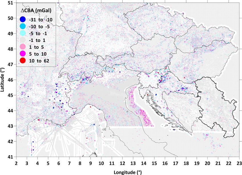
2166                                                              P. Zahorec et al.: The first pan-Alpine surface-gravity database

       for the Ivrea zone in the Western Alps, recently acquired data were added to the database. This first pan-Alpine
       gravity data map is homogeneous regarding input data sets, applied methods and all corrections, as well as
       reference frames.
          Here, the AAGRG presents the data set of the recalculated gravity fields on a 4 km × 4 km grid for public
       release and a 2 km × 2 km grid for special request. The final products also include calculated values for mass and
       bathymetry corrections of the measured gravity at each grid point, as well as height. This allows users to use later
       customized densities for their own calculations of mass corrections. Correction densities used are 2670 kg m−3
       for landmasses, 1030 kg m−3 for water masses above the ellipsoid and −1640 kg m−3 for those below the ellip-
       soid and 1000 kg m−3 for lake water masses. The correction radius was set to the Hayford zone O2 (167 km).
       The new Bouguer anomaly is station completed (CBA) and compiled according to the most modern criteria and
       reference frames (both positioning and gravity), including atmospheric corrections. Special emphasis was put on
       the gravity effect of the numerous lakes in the study area, which can have an effect of up to 5 mGal for gravity
       stations located at shorelines with steep slopes, e.g., for the rather deep reservoirs in the Alps. The results of an
       error statistic based on cross validations and/or “interpolation residuals” are provided for the entire database. As
       an example, the interpolation residuals of the Austrian data set range between about −8 and +8 mGal and the
       cross-validation residuals between −14 and +10 mGal; standard deviations are well below 1 mGal. The accuracy
       of the newly compiled gravity database is close to ±5 mGal for most areas.
          A first interpretation of the new map shows that the resolution of the gravity anomalies is suited for ap-
       plications ranging from intra-crustal- to crustal-scale modeling to interdisciplinary studies on the regional and
       continental scales, as well as applications as joint inversion with other data sets. The data are published with the
       DOI https://doi.org/10.5880/fidgeo.2020.045 (Zahorec et al., 2021) via GFZ Data Services.

1   Introduction                                                      Götze, 1978; Kissling, 1980; Götze and Lahmeyer, 1988;
                                                                      Götze et al., 1991; Ebbing, 2002; Ebbing et al., 2006; Mar-
There is a long history of geological and geophysical re-             son and Klingelé, 1993; Kahle and Klingelé, 1979). How-
search on the Alpine orogen, the results of which point to            ever, these land data sets for historical reasons were acquired
two main groups of complexity. The first is the temporal evo-         in national reference systems and were seldom shared, pre-
lution of the mountain belt, with plates, terrains and units of       venting high-resolution pan-Alpine gravity studies using ho-
different size and level of deformation mostly investigated           mogeneously processed data.
from the geological record (e.g., Handy et al., 2010). This
inheritance directly influences the second level of complex-          1.1   The AlpArray Gravity Research Group
ity, which is structural and characterizes every level of the
lithosphere from sedimentary basins to orogenic roots and             With respect to the national expertise and databases available
also the upper mantle. The level of along-strike variability          in the Alpine countries, the formation of an international re-
of the Alps exceeds what is known in other mountain belts             search group (AlpArray Gravity Research Group; AAGRG)
such as the Andes and the Himalayas (Oncken et al., 2006;             was decided within the framework of activities in the Euro-
Hetényi et al., 2016) and explains why some of the orogenic           pean AlpArray program and established at an EGU splinter
processes operating in the Alps are still debated.                    meeting in 2017. In the subsequent workshops in Bratislava
   Structural complexity at depth, and thus the advancement           (Slovakia) in 2018, and two further technical meetings of the
of our understanding of orogeny, can be resolved by high-             group (again in Bratislava in 2018 and in Sopron, Hungary, in
resolution 3D geophysical imaging. This is among the pri-             2019), the organizational, scientific, and numerical require-
mary goals of the AlpArray program and its main seismolog-            ments for the compilation of the new pan-Alpine digital grav-
ical imaging tool, the AlpArray Seismic Network. This mod-            ity database were established, which consists of Bouguer and
ern array has used over 628 sites for more than 39 months             free-air anomalies (BA and FA) and values of mass correc-
across the greater Alpine area such that no point on land was         tion. Although most of the national group members were
farther than 30 km from a broadband seismometer (Hetényi              extensively involved in the processing of data, we would
et al., 2018). While seismic imaging of the entire Alps in 3D         like to remind with gratitude that by far the most intensive
became a reality following decades of active- and passive-            part of the processing was done by the group members from
source projects, imaging efforts in gravity reached 3D earlier        Bratislava and Banská Bystrica (Slovakia).
thanks to the availability of national data sets of the Alpine           In the following, we present our effort, omitting historical
neighboring countries with partly high-resolution and 3D              obstacles, in compiling and merging all available land and
modeling approaches among others (Ehrismann et al., 1976;             sea gravity data in the greater Alpine area, a total of more

Earth Syst. Sci. Data, 13, 2165–2209, 2021                                            https://doi.org/10.5194/essd-13-2165-2021
The first pan-Alpine surface-gravity database, a modern compilation that crosses frontiers - ESSD
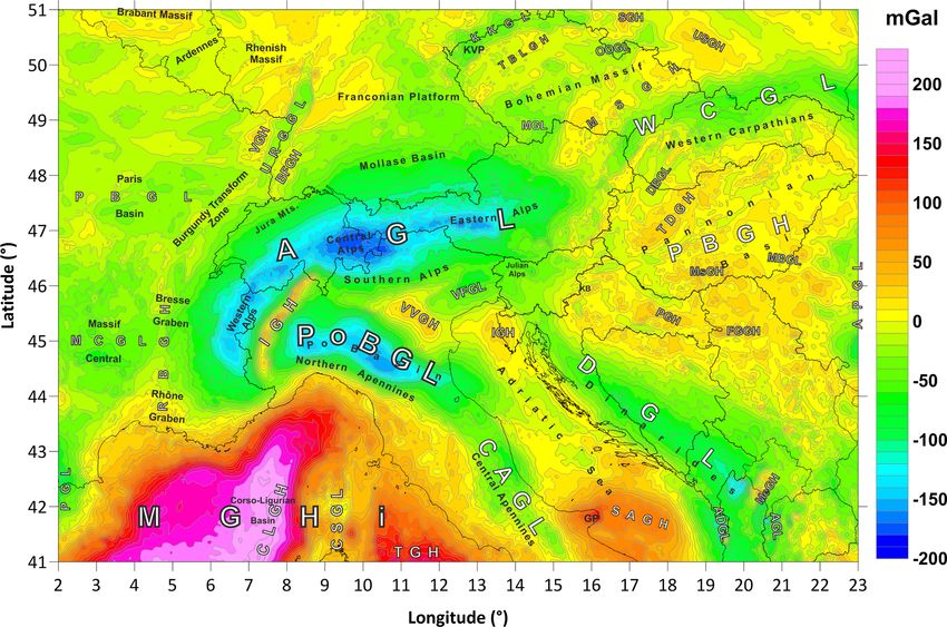
P. Zahorec et al.: The first pan-Alpine surface-gravity database                                                              2167

than 1 million on- and offshore data points. We committed           2.1   Problems with positioning, heights and gravity data
to the exact same data processing procedures so that even
proprietary point-wise data can be included at the project’s        One of the key problems in the unification of gravimet-
initial stage and represented in the final Bouguer anomaly          ric databases is the homogenization of position, height
grids.                                                              and gravimetric coordinate systems used in each database.
   We emphasize that the data set is primarily a product to         Through its historical development, each country has used
be used for an interdisciplinary 3D modeling of the Earth’s         and sometimes still uses local systems and their realization
lithosphere which requires precise mass corrections, consid-        (frame), which are often based on the established principles
ering topography, bathymetry and onshore lake corrections.          of reference systems using older ellipsoids or older geode-
Therefore, it differs significantly from modern gravity poten-      tic reference networks and projections. These systems and
tial field compilations which aim at geoid and quasi-geoid          their realizations thus contain several differences which are
modeling (e.g., Denker, 2013). Here, we focus on providing          responsible for large inhomogeneities, shifts and errors in po-
a valuable data set for numerous interdisciplinary projects         sition, height and gravity. These errors are most evident in the
in the AlpArray program and other European geo-projects             mutual comparison of data from individual countries.
that support crustal and mantle modeling in the Alpine-                To avoid these problems in the position of gravimetric
Mediterranean region.                                               points, all position data were transformed from local sys-
                                                                    tems to the European Terrestrial Reference System 1989
1.2    Publication layout                                           (ETRS89), which is accurate, homogeneous and recom-
                                                                    mended for all European countries (Altamimi, 2018). A sim-
We document in detail our procedures, from raw data to fi-          ilar situation is in the height systems in that countries use
nal high-resolution gravity maps. The referencing and quality       different types of physical heights, they are linked to differ-
assessment of various gravity databases and digital Earth sur-      ent tide gauges, and each country has a different practical
face models are discussed in Sect. 2. The equations and their       implementation of the relevant height system. The solution
implementations to obtain various gravity anomaly products,         is again the transformation to a uniform platform in the form
as well as the reprocessing of original raw data and of the re-     of ellipsoidal heights in the ETRS89 system based on the
lated corrections, are described in Sect. 3. Section 4 presents     ellipsoid GRS80 (Moritz, 2000). The situation is similar in
the new, homogenized Bouguer gravity map for the Alps. In           gravimetric reference systems, in which especially the gravi-
Sect. 4.3 we describe the attached Bouguer map, together            metric databases that have been created for decades often use
with an accompanying description and interpretation of the          old gravimetric systems linked to the Potsdam system. An
gravity anomalies in the Alps and their surroundings. Notes         important step was therefore to convert these data into gravi-
on the uncertainty of the compilation are given in Sect. 5.         metric systems which are connected to absolute gravimetric
We conclude on the listing and availability of the new grav-        points and measurements, such as IGSN71 (Morelli et al.,
ity data (Sect. 6), which we share publicly as a contribution       1972) or modern national systems connected with the recent
to further gravity studies in the region at different scales.       absolute measurements, which are verified by international
   Additionally, information is provided in four appendices         comparisons of absolute gravimeters (Francis et al., 2015).
for detailed descriptions of national data sets, procedures,           For these transformations, national transformation ser-
strategies and comparisons. Appendix A contains a list of ab-       vices were used (operated by national mapping services, e.g.,
breviations used; Appendix B gives a brief overview of the          SAPOS, SKPOS) or transformations implemented into stan-
historical activities of the main actors and the national contri-   dard GIS tools or our own software implementations based
butions to the pan-Alpine Bouguer gravity map; Appendix C           on national standards, information and experience of individ-
presents and compares the digital elevation models (DEMs)           ual responsible institutions. The transformation from physi-
used; and finally, Appendix D provides details on the mass          cal heights in national vertical systems to ellipsoidal heights
correction (MC) software and compares MC gravity effects            in the ETRS89 system, ellipsoid GRS80, was realized us-
resulting from different DEMs.                                      ing available local geoid and quasi-geoid models available
                                                                    through transformation services or implemented in current
2     Assessment of database                                        geodetic processing programs (e.g., Trimble Business Cen-
                                                                    ter, Leica Infinity). If a local geoid or quasi-geoid model was
In total, all gravity data sets used comprise 1 008 815 grav-       not available for some areas, then the global geopotential
ity stations. Figure 1 shows the spatial distribution of the        model EIGEN-6C4 (Förste et al., 2014) was used for trans-
original data sets country by country. The initial situation        formation. This model was also used for marine data, for
for the assessment and application of existing data, available      which the height of points was not given or had zero value.
publications, data density and quality description is provided         Provided data include a local identifier, horizontal co-
country by country in Appendix B.                                   ordinates in the local coordinate systems (except France
                                                                    and Croatia), physical height, ellipsoidal coordinates in the
                                                                    ETRS89 system, ellipsoidal height above the GRS80 ellip-

https://doi.org/10.5194/essd-13-2165-2021                                          Earth Syst. Sci. Data, 13, 2165–2209, 2021
The first pan-Alpine surface-gravity database, a modern compilation that crosses frontiers - ESSD
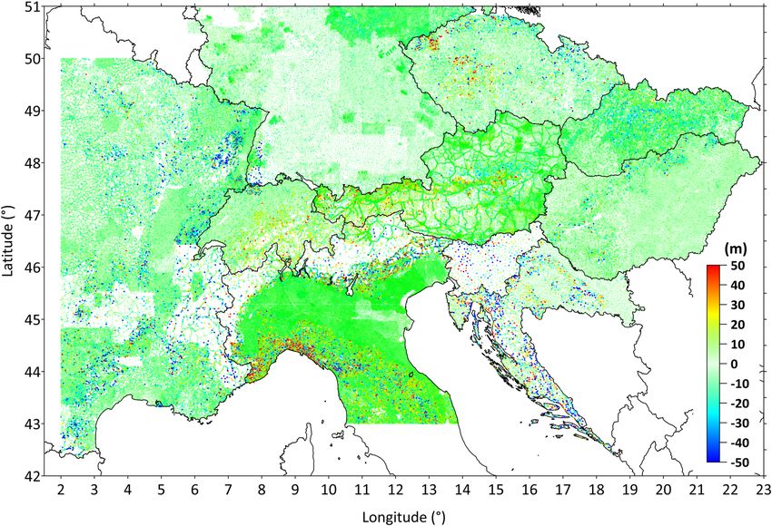
2168                                                                 P. Zahorec et al.: The first pan-Alpine surface-gravity database

Figure 1. The distribution of more than 1 million gravity stations in the area of investigation and compilation. Colors indicate the national
databases used in the compilation.

soid (except France, the Czech Republic and Slovenia) and
the gravity value. For each parameter available metadata de-
scribing, for example, coordinate system (ellipsoid, EPSG
code), transformation method or transformation service used,
and local geoid and quasi-geoid were also collected.
   Figure 2 shows the transformation scheme. For data sets
for which all information was available, an independent
transformation control check was performed between the lo-
cal and global coordinate systems and between physical and
ellipsoidal heights using available geodetic geoid and quasi-
geoid models. Differences in position were in the majority
of cases less than 1 m. All larger differences were individu-
ally investigated. A similar situation was for the heights, for
which differences were generally less than 50 cm. These dif-
ferences were mostly caused by different transformations, its            Figure 2. Transformation scheme for unification of the national po-
practical software realization or local specifics of the data set.       sitioning, height and gravity reference systems.
   Data statistics and an overview of selected metadata are
given in Table 1.
                                                                         3   Reprocessing of original data and applied
                                                                             corrections
2.2    Digital elevation models
                                                                         Both the new complete Bouguer anomaly (CBA) and the
One of the important elements in the calculation of com-                 free-air anomaly of the studied region were calculated for
plete Bouguer anomaly (CBA) is the calculation of proper                 ellipsoidal heights of calculation points with their geograph-
mass corrections. The prerequisite for the calculation of cor-           ical coordinates (λ, ϕ). For CBA mass corrections (gravita-
rect gravity effects of topographic masses is the use of high-           tional effects of masses) δgM extending to the standard dis-
resolution digital terrain models (DTMs). Further informa-               tance of 166.7 km, bathymetric corrections δgB and simpli-
tion on the availability and use of DEMs in the Alpine area              fied atmospheric corrections δgA were applied. In contrast
is given in Appendix C.                                                  to the conventional processing of Bouguer gravity, a mass

Earth Syst. Sci. Data, 13, 2165–2209, 2021                                                https://doi.org/10.5194/essd-13-2165-2021
The first pan-Alpine surface-gravity database, a modern compilation that crosses frontiers - ESSD
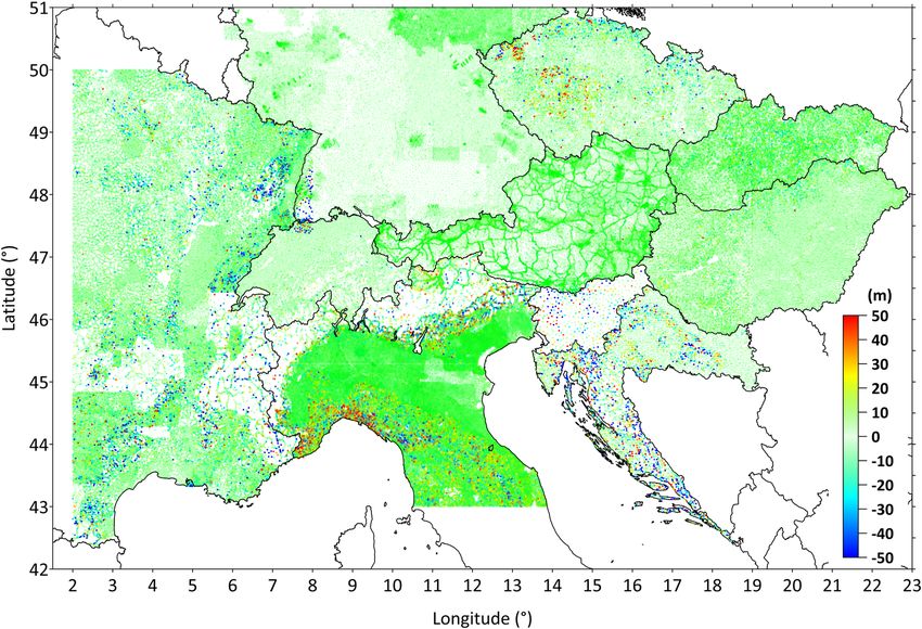
P. Zahorec et al.: The first pan-Alpine surface-gravity database                                                                                                                                                                                                                                                                                                                                                                                       2169

                                                                                                                                                                                                                                                                                                                                           Zahorec et al. (2017b); ZBGIS (2020)
                                                                                                                                                                                                                                                                                                                                                                                              correction was calculated for masses between the ellipsoidal
       Table 1. Data statistics and an overview of selected metadata. From the total of originally 1 076 871 gravity stations, 1 008 815 data points were used for the compilation of the gravity

                                                                                                                                                                                                                                                                                                                                           Olivier et al. (2010); Marti (2007)
                                                                                                                                                                                                                                                                                                                                                                                              reference surface and the physical surface (Sect. 3.1). In ad-
                                                                                                                                                                                                                                                                                                                                                                                              dition, emphasis was put on the calculation of the gravimetric

                                                                                                                                                                                                                                                                                                                                           Bašić and Bjelotomi (2014)
                                                                                                                                                                                                                                                                                                                                                                                              effects of the Alpine lakes on the basis of bathymetric data

                                                                                                                                                                                                                                                                                                                                           Kostelecky et al. (2004)

                                                                                                                                                                                                                                                                                                                                           Bilibajkič et al. (1979)
                                                                                                                                                                                                                                                                                                                                                                                              of the region (Sect. 3.2). To complete the AAGRG database

                                                                                                                                                                                                                                                                                                                                           Barzaghi et al. (2007)
                                                                                                                                                                                                                                                                                                                                           Schwabe et al. (2016)
                                                                                                                                                                                                                                                                                            Notes and references

                                                                                                                                                                                                                                                                                                                                           Kuhar et al. (2011)
                                                                                                                                                                                                                                                                                                                                                                                              an old CBA map from the former Socialist Federal Republic

                                                                                                                                                                                                                                                                                                                                           BGI, archive data
                                                                                                                                                                                                                                                                                                                                           Pail et al. (2008)

                                                                                                                                                                                                                                                                                                                                           VITEL (2020)
                                                                                                                                                                                                                                                                                                                                                                                              (SFR) of Yugoslavia (Bilibajkič et al., 1979) (Sect. 3.3) was

                                                                                                                                                                                                                                                                                                                                           IGN (2010)
                                                                                                                                                                                                                                                                                                                                                                                              digitized. Further improvements of the new CBA map are
                                                                                                                                                                                                                                                                                                                                                                                              the refined calculations of an atmospheric correction and the
                                                                                                                                                                                                                                                                                                                                                                                              future containment of distant terrain and bathymetry effects
                                                                                                                                                                                                                                                                                                                                                                                              (Sect. 3.4).
                                                                                                                                                                                                                                                                                                                                           Potsdam/IGSN71
                                                                                                                                                                                                                                                                                                                                           ABS MGH-2000
                                                                                                                                                                                                                                                                                                                                                                                                 The basic formula for the CBA calculation was adopted

                                                                                                                                                                                                                                                                                                                                           ABS LSN2004
                                                                                                                                                                                                                                                                                                                                                                                              from Meurers et al. (2001):
                                                                                                                                                                                                                                                                                                                                           ABS Sgr95

                                                                                                                                                                                                                                                                                                                                           ABS Sgr95
                                                                                                                                                                                                                                                                                                                                           IGSN71

                                                                                                                                                                                                                                                                                                                                           IGSN71

                                                                                                                                                                                                                                                                                                                                           IGSN71
                                                                                                                                                                                                                                                                                            Gravity
                                                                                                                                                                                                                                                                                                                   g value

                                                                                                                                                                                                                                                                                                                                           CBA                                                BA(λ, ϕhE ) =g(λ, ϕhE ) − γ (ϕhE ) − δgM (λ, ϕhE )
                                                                                                                                                                                                                                                                                                                                           FA
                                                                                                                                                                                                                                                                                                                                           x

                                                                                                                                                                                                                                                                                                                                           x

                                                                                                                                                                                                                                                                                                                                                                                                                 + δgB (λ, ϕ, H ) + δgA (λ, ϕ, H ),      (1)
                                                                                                                                                                                                                                                                                                                   Ellipsoid

                                                                                                                                                                                                                                                                                                                                                                                                                      ∂γ          1    ∂ 2γ
                                                                                                                                                                                                                                                                                                                                                                                              γ (ϕhE ) = γ0 (ϕ) +         |0 hE +       |0 h2 ,          (2)
                                                                                                                                                                                                                                                                                                                                                                                                                      ∂hE         2 ∂h2E E
                                                                                                                                                                                                                                                                                                                                           x
                                                                                                                                                                                                                                                                                                                                           x
                                                                                                                                                                                                                                                                                                                                           –
                                                                                                                                                                                                                                                                                                                                           –
                                                                                                                                                                                                                                                                                                                                           x
                                                                                                                                                                                                                                                                                                                                           x
                                                                                                                                                                                                                                                                                                                                           x
                                                                                                                                                                                                                                                                                                                                           x
                                                                                                                                                                                                                                                                                                                                           –
                                                                                                                                                                                                                                                                                                                                           x
                                                                                                                                                                                                                                                                                                                                           –
                                                                                                                                                                                                                                                                                                                                           –
                                                                                                                                                                                                                                                                                                                   Geoid and quasi-geoid

                                                                                                                                                                                                                                                                                                                                                                                              where γ0 (ϕ) results from the well-known Somigliana for-
                                                                                                                                                                                                                                                                                                                                                                                              mula (Somigliana, 1929) for the normal gravity acceleration
                                                                                                                                                                                                                                                                                                                                           SLOAMG2000
                                                                                                                                                                                                                                                                                                                                           BEV GV 2008

                                                                                                                                                                                                                                                                                                                                           ITALGEO05

                                                                                                                                                                                                                                                                                                                                           CHGEO04A

                                                                                                                                                                                                                                                                                                                                                                                              of a rotational ellipsoid at its surface (Heiskanen and Moritz,
                                                                                                                                                                                                                                                                                                                                           VITEL2014

                                                                                                                                                                                                                                                                                                                                           EIGEN6C4
                                                                                                                                                                                                                                                                                                                                           EIGEN6C4
                                                                                                                                                                                                                                                                                                                                           HRG2009

                                                                                                                                                                                                                                                                                                                                           GCG2016

                                                                                                                                                                                                                                                                                                                                           DVRM05
                                                                                                                                                                                                                                                                                                                                           CR-2005

                                                                                                                                                                                                                                                                                                                                                                                              1967):
                                                                                                                                                                                                                                                                                                                                           RAF09
                                                                                                                                                                                                                                                                                            Height

                                                                                                                                                                                                                                                                                                                                                                                                      a γE cos2 ϕ + c γP sin2 ϕ
                                                                                                                                                                                                                                                                                                                                                                                              γ0 (ϕ) = p                        ,                        (3)
                                                                                                                                                                                                                                                                                                                                                                                                         a 2 cos2 ϕ + c2 sin2 ϕ
                                                                                                                                                                                                                                                                                                                                           Kronstadt Baltic height system

                                                                                                                                                                                                                                                                                                                                           Kronstadt Baltic height system

                                                                                                                                                                                                                                                                                                                                           Kronstadt Baltic height system

                                                                                                                                                                                                                                                                                                                                                                                              and higher vertical derivatives of γ (ϕ, hE ) are given by
                                                                                                                                                                                                                                                                                                                                           Amsterdam DHHN
                                                                                                                                                                                                                                                                                                                                           Trieste HVRS1971

                                                                                                                                                                                                                                                                                                                                                                                                               
                                                                                                                                                                                                                                                                                                                                                                                               ∂γ          2γ0                           3
                                                                                                                                                                                                    maps. Most of the points were eliminated during the post-processing of offshore data.

                                                                                                                                                                                                                                                                                                                                           Marseille LN02

                                                                                                                                                                                                                                                                                                                                                                                                     = −         1 + f − 2 f sin2 ϕ + f 2
                                                                                                                                                                                                                                                                                                                                                                                               ∂hE 0        a                            2
                                                                                                                                                                                                                                                                                                                                           Marseille
                                                                                                                                                                                                                                                                                                                   Physical

                                                                                                                                                                                                                                                                                                                                                                                                                                    
                                                                                                                                                                                                                                                                                                                                                                                                                        1
                                                                                                                                                                                                                                                                                                                                           Trieste

                                                                                                                                                                                                                                                                                                                                           Trieste
                                                                                                                                                                                                                                                                                                                                           Genoa

                                                                                                                                                                                                                                                                                                                                                                                                       −2f 2 sin2 ϕ + f 2 sin4 ϕ − 2ω2 ,
                                                                                                                                                                                                                                                                                                                                           Zero

                                                                                                                                                                                                                                                                                                                                                                                                                                                         (4)
                                                                                                                                                                                                                                                                                                                                                                                                                        2
                                                                                                                                                                                                                                                                                                                                           –

                                                                                                                                                                                                                                                                                                                                                                                              ∂ 2γ                  6γ0
                                                                                                                                                                                                                                                                                                                   ETRS89

                                                                                                                                                                                                                                                                                                                                                                                                         =                      2 .                     (5)
                                                                                                                                                                                                                                                                                                                                                                                              ∂h2E   0       a 2 1 − f sin2 ϕ
                                                                                                                                                                                                                                                                                                                                           x
                                                                                                                                                                                                                                                                                                                                           x
                                                                                                                                                                                                                                                                                                                                           x
                                                                                                                                                                                                                                                                                                                                           x
                                                                                                                                                                                                                                                                                                                                           x
                                                                                                                                                                                                                                                                                                                                           –
                                                                                                                                                                                                                                                                                                                                           x
                                                                                                                                                                                                                                                                                                                                           x

                                                                                                                                                                                                                                                                                                                                                                      x
                                                                                                                                                                                                                                                                                                                                                                      –
                                                                                                                                                                                                                                                                                                                                                                      x
                                                                                                                                                                                                                                                                                                                                           Oblique Mercator LV03

                                                                                                                                                                                                                                                                                                                                                                                              All constants in Eqs. (3) to (5) were taken from the Geodetic
                                                                                                                                                                                                                                                                                            Position

                                                                                                                                                                                                                                                                                                                                                                                              Reference System 1980 (GRS80), e.g., in Moritz (1984):
                                                                                                                                                                                                                                                                                                                                           Gauß–Krüger D-48
                                                                                                                                                                                                                                                                                                                                           Gauß–Krüger S-42

                                                                                                                                                                                                                                                                                                                                           Gauß–Krüger S-42
                                                                                                                                                                                                                                                                                                                                           Krovak S-JTSK

                                                                                                                                                                                                                                                                                                                                                                                                – γE = 9.7803267715 m s−2 , normal gravity acceleration
                                                                                                                                                                                                                                                                                                                                                                                                  at the Equator,
                                                                                                                                                                                                                                                                                                                   National

                                                                                                                                                                                                                                                                                                                                           UTM32
                                                                                                                                                                                                                                                                                                                                           EOV
                                                                                                                                                                                                                                                                                                                                           MGI

                                                                                                                                                                                                                                                                                                                                                                                                – γP = 9.8321863685 m s−2 , normal gravity acceleration
                                                                                                                                                                                                                                                                                                                                           –

                                                                                                                                                                                                                                                                                                                                           –

                                                                                                                                                                                                                                                                                                                                           –

                                                                                                                                                                                                                                                                                                                                           –

                                                                                                                                                                                                                                                                                                                                                                                                  at pole,
                                                                                                                                                                                                                                                                                            Number of points
                                                                                                                                                                                                                                                                                                                   All/used
                                                                                                                                                                                                                                                                                                                                             54 251/51 811
                                                                                                                                                                                                                                                                                                                                                4939/4565
                                                                                                                                                                                                                                                                                                                                             13 955/13 831
                                                                                                                                                                                                                                                                                                                                             58 750/57 889
                                                                                                                                                                                                                                                                                                                                             36 442/36 440
                                                                                                                                                                                                                                                                                                                                             25 434/25 147
                                                                                                                                                                                                                                                                                                                                           132 074/130 821
                                                                                                                                                                                                                                                                                                                                             21 108/21 108
                                                                                                                                                                                                                                                                                                                                                 3066/364
                                                                                                                                                                                                                                                                                                                                                7962/7962

                                                                                                                                                                                                                                                                                                                                                                            718 890/658 877

                                                                                                                                                                                                                                                                                                                                                                                                – a = 6 378 137 m, semi-major axis of the normal ellip-
                                                                                                                                                                                                                                                                                                                                                                                                  soid,

                                                                                                                                                                                                                                                                                                                                                                                                – c = 6 356 752.3141 m, semi-minor axis of the normal
                                                                                                                                                                                                                                                                                                                                                                                                  ellipsoid,
                                                                                                                                                                                                                                                                                                                                           Former Yugoslavia
                                                                                                                                                                                                                                                                                                                                           Czech Republic

                                                                                                                                                                                                                                                                                                                                                                                                – f = 0.00335281068118, geometrical flattening,
                                                                                                                                                                                                                                                                                                                                           Switzerland
                                                                                                                                                                                                                                                                                                                                           Germany
                                                                                                                                                                                                                                                                                                                                           Hungary

                                                                                                                                                                                                                                                                                                                                           Slovenia
                                                                                                                                                                                                                                                                                                                                           Slovakia
                                                                                                                                                                                                                                                                                                                                           Austria
                                                                                                                                                                                                                                                                                                                                           Croatia

                                                                                                                                                                                                                                                                                                                                           Marine

                                                                                                                                                                                                                                                                                                                                                                                                – ω = 7.292115 ×10⁻⁵ rad s−1 , angular velocity of the
                                                                                                                                                                                                                                                                                                                                           France

                                                                                                                                                                                                                                                                                                                                           Italy

                                                                                                                                                                                                                                                                                                                                                                                                  Earth’s rotation.

https://doi.org/10.5194/essd-13-2165-2021                                                                                                                                                                                                                                                                                                                                                                        Earth Syst. Sci. Data, 13, 2165–2209, 2021
The first pan-Alpine surface-gravity database, a modern compilation that crosses frontiers - ESSD
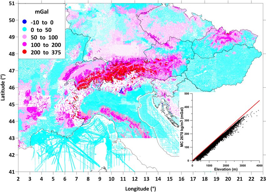
2170                                                                  P. Zahorec et al.: The first pan-Alpine surface-gravity database

Simplified atmospheric corrections δgA (Wenzel, 1985) were
calculated by means of the approximation

δgA (λ, ϕ, H ) = 0.874 − 9.9 × 10⁻⁵ H + 3.56 × 10⁻⁹ H 2 (6)

(δgA in mGal1 , H in meters).
   From a methodological viewpoint, the use of ellipsoidal
heights for CBA calculation is innovative. Considering the
participating countries, so far this concept has only been
used in Austria (Meurers and Ruess, 2009). It ensures that
Bouguer anomalies, which then, in the sense of physical
geodesy, actually are gravity disturbances corrected for ter-
rain mass effects, are not disturbed by the geophysical in-
direct effect (GIE; e.g. Li and Götze, 2001; Hackney and
Featherstone, 2003) contrary to Bouguer anomalies relying
on physical heights.

3.1    Mass correction
One of the main problems in the homogenization of data
and recompilation of gravity fields was the use of dif-
ferent procedures for the calculation of mass correction
(MC) and bathymetry correction (BC) by national opera-
tors/authorities. This meant that a complete recalculation had
to be carried out for the new compilation based on the avail-             Figure 3. Schematic comparison of physical vs. ellipsoidal concept
able point data and the best digital elevation models (DEMs)              of CBA. Note that the effect of additional water masses is calculated
available. The proper choice of DEMs is discussed in Ap-                  in a two-step process.
pendix C. An important first step before starting the recom-
pilation was to test and select the available software to cal-
culate the mass corrections. We compared two custom soft-
                                                                          layer of topography whose effect is calculated in the same
ware packages developed by team members: Toposk soft-
                                                                          way as in the case of physical heights (with the density of
ware (Zahorec et al., 2017a) and TriTop (Holzrichter et al.,
                                                                          2670 kg m−3 ). In the case of marine areas, the situation is
2019). Considering the results of this comparison (refer to
                                                                          somewhat more complicated as the ocean masses are partly
Appendix D), we decided to use Toposk based on ellipsoidal
                                                                          above the ellipsoid level. If we want to take these into ac-
heights hE of the calculation points and ellipsoidal digital el-
                                                                          count with their real density (1030 kg m−3 ), it is necessary
evation models (using in the majority of cases local geoids
                                                                          to separate their effect from terrain masses. Numerically, this
for the transformation). On the other hand, the bathymet-
                                                                          can be done by taking these water masses into account first
ric and simplified atmospheric corrections were calculated
                                                                          as topographic masses (i.e., with a density of 2670 kg m−3 )
for physical heights H of the calculation points. Bathymetric
                                                                          and then also as part of the bathymetric correction (i.e., with
corrections were also calculated by means of the Toposk soft-
                                                                          a density of −1640 kg m−3 ). As a result, we assign a den-
ware but in a slightly adjusted mode (see below and Fig. 3).
                                                                          sity ρ of 1030 kg m−3 to these water masses (ρ = 2670–
   If the normal field in Eq. (1) is defined at the height
                                                                          1640 kg m−3 ).
above the surface ellipsoid, it is necessary to define the ef-
                                                                             In connection with the above calculation methods, one
fects of terrain and bathymetry masses above the ellipsoid
                                                                          note is appropriate. The difference between the two versions
(not above the geoid). Therefore, the concept requires the
                                                                          (physical vs. ellipsoidal heights) of the CBA defines GIE,
use of ellipsoidal heights of the observation points, and at
                                                                          which has a normal gravity component (defined by the free-
the same time it is necessary to transform the topography
                                                                          air gradient) and a component defined by the gravitational
and bathymetry grids from physical to ellipsoidal heights.
                                                                          attraction of the masses between the geoid and the ellipsoid.
In the AlpArray area, the situation is more or less simple,
                                                                          In our case, this second component is equal to the total gravi-
the ellipsoid is below the geoid throughout the region (ap-
                                                                          tational effect of these masses with a density of 2670 kg m−3
prox. 30 to 55 m). This greatly simplifies the calculation.
                                                                          (no difference in density at sea and on land). This is in ap-
In the case of continental areas, we get a slightly thicker
                                                                          parent contradiction to published papers which state that the
   1 Note: though different from the SI units, we will use the unit       GIE should be calculated with different densities for land
mGal for gravity, which is still frequently used in gravimetry;           and sea (offshore with a density of 1030 kg m−3 ). This appar-
1 mGal = 10−5 m s−2 .                                                     ent discrepancy is due to different approaches to bathymetric

Earth Syst. Sci. Data, 13, 2165–2209, 2021                                                 https://doi.org/10.5194/essd-13-2165-2021
The first pan-Alpine surface-gravity database, a modern compilation that crosses frontiers - ESSD
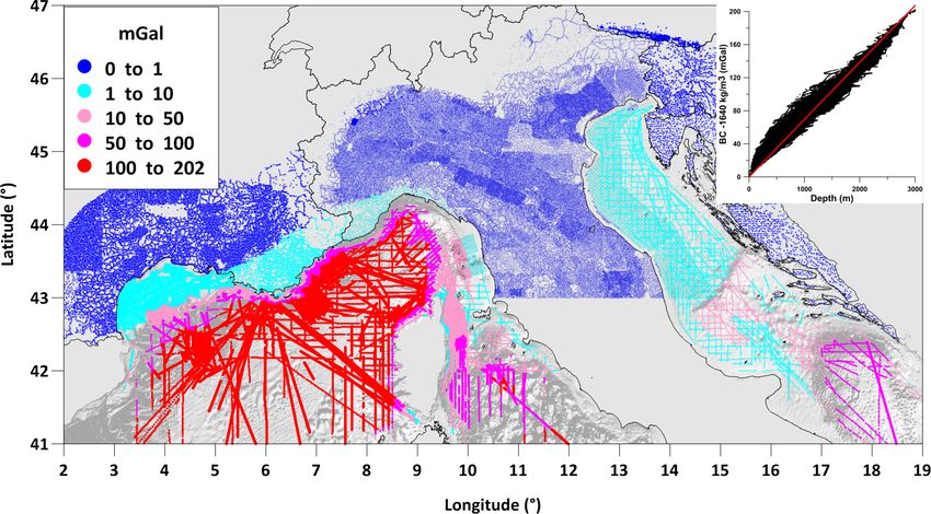
P. Zahorec et al.: The first pan-Alpine surface-gravity database                                                             2171

correction. The approach of Chapman and Bodine (1979) is              For many large lakes in Switzerland bathymetric surveys
based on free-air anomalies which do not include bathymet-         have been carried out since 2007 (Urs Marti, personal com-
ric corrections, unlike our CBA. The GIE is thus easier to         munication, 2019). The resolution of these models varies
define in our case (for a constant density of 2670 kg m−3 in       between 1 and 3 m. For all the other lakes which contain
the whole space considered between the geoid and the ellip-        bathymetric contours in the topographic map at a scale of
soid) thanks to the consideration of the rock–water density        1 : 25 000, these contours have been digitized and interpo-
contrast in this space as part of the bathymetric correction.      lated to grids at a resolution of 25 m.
   Figure 4 visualizes the MC values at all collected points.         In Slovenia there are two big Alpine lakes of glacial ori-
They reach values up to 375 mGal, while the ellipsoidal            gin located in the Julian Alps in the northwestern part of the
height of the points is from about 35 to 3938 m. The height        country. For both lakes, high-resolution bathymetric data are
dependence of the calculated MC is displayed in the lower          available. Bathymetric surveys were performed in the years
right corner of the figure. The difference between the calcu-      2015–2017 (Harpha Sea, 2017). The maximum depths for
lated MC and the gravitational effect of the truncated spheri-     Lake Bohinj and Lake Bled are 45 and 30 m, respectively.
cal layer (to the same distance) defines classic terrain correc-   The bathymetric grid size of 20 m was used to compute the
tions. They reach values of almost 100 mGal.                       Alpine lake corrections for the new CBA.
                                                                      No digital depth information was available for Austrian
3.2     Bathymetric and lake correction                            lakes. Therefore, shorelines and bathymetric contour lines
                                                                   have been digitized from topographic maps and interpolated
3.2.1    Bathymetric corrections                                   to grids with 10 m spacing. All lakes (in total 36) exceeding
When calculating bathymetric corrections (BCs), the grav-          either a water volume of 25 × 106 m3 or maximum depth of
ity effect is calculated due to the difference in density be-      50 m have been handled in this way, including artificial reser-
tween the water masses of the offshore areas and those of          voirs. The altitude of the lake level surfaces was derived from
the land masses. In contrast to the MC, we calculate BC            topographic maps too. Seasonal lake level variations cannot
with physical heights as explained in Sect. 3.1 and Fig. 3.        be ruled out; however, they are expected to be less than 1–2 m
Water masses above the ellipsoid level are thus considered         for natural lakes. The situation may be worse for reservoirs.
with their real density of 1030 kg m−3 . We used a detailed           The depth data for lakes in the German parts of the North-
bathymetric model EMODnet (EMODnet Bathymetry Con-                 ern Alps was digitized from topographic maps at a scale of
sortium, 2018) with the resolution of 3.75 arcsec. A har-          1 : 50 000. The resolution is 25 m or 1 arcsec. Vertical heights
monized DEM has been generated for European offshore               are physical (normal) heights.
regions from selected bathymetric survey data sets, com-              The models mentioned were combined with existing de-
posite digital terrain models (DTMs) and satellite-derived         tailed DEMs, and the lake correction itself was calculated
bathymetry (SDB) data products, while gaps with no data            as the difference of the gravitational effects of two topog-
coverage were completed by integrating the GEBCO digital           raphy models, one containing the level of the lakes and the
bathymetry (GEBCO Compilation Group, 2020).                        other their bottom (e.g., Fig. 6 for Lake Geneva). Calculated
   Bathymetric corrections reach significant values for off-       lake corrections (density 1670 kg m−3 ) for all countries with
shore and near coastal points and amount to more than              available lake models are shown in Fig. 7. The corrections
200 mGal (Fig. 5). The comparison with the frequently used         reach maximum values of about 5 mGal, especially on the
planar approximation is in the upper right corner of the fig-      lakesides with steep mountain flanks.
ure. Unlike MC (refer to Fig. 4), these differences are not
systematic and reach about ±30 mGal.                               3.3   Digitization and reprocessing of the CBA map of the
                                                                         former SFR Yugoslavia
3.2.2    Lake corrections
                                                                   Although the peripheral southeastern part of the new
Because the DEMs used in the MC calculation also include           Bouguer gravity map is not covered by terrestrial data which
the volumes of water masses of Alpine lakes, these volumes         were available to the project, this area was filled by the dig-
are calculated with an incorrect density (2670 instead of          itization of the CBA map of the former SFR Yugoslavia at a
1000 kg m−3 ). We can eliminate this discrepancy by the ap-        scale of 1 : 500 000 (Bilibajkič et al., 1979). The CBA map
plication of a lake correction. Steinhauser et al. (1990) point    (with a correction density of 2670 kg m−3 ) was published
out that some Alpine lakes reach a depth of up to 300 m and,       in 1972 and covers the whole area of the former SFR Yu-
due to easy accessibility, gravity stations are frequently lo-     goslavia. Its northern part was converted into an electronic
cated close to lake shores. An important prerequisite for a        form in the diploma thesis of Grand (2019). For the needs
correct calculation is the availability of adequate models of      of the AlpArray project, a map was used especially for the
lake bottoms. Except for Italy, depth models were available        territory of Serbia and Bosnia and Herzegovina. The gravity
for four countries: for Switzerland, Austria, Germany and          data of Slovenia and Croatia were also originally part of the
Slovenia.                                                          Yugoslavian gravity map (refer to Appendix B – Croatia). In

https://doi.org/10.5194/essd-13-2165-2021                                         Earth Syst. Sci. Data, 13, 2165–2209, 2021
The first pan-Alpine surface-gravity database, a modern compilation that crosses frontiers - ESSD
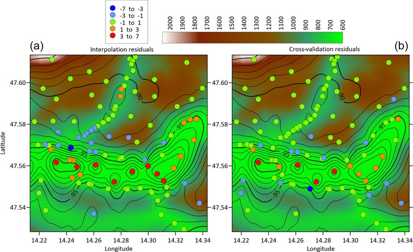
2172                                                               P. Zahorec et al.: The first pan-Alpine surface-gravity database

Figure 4. Map of mass correction (up to the distance of 166 730 m, density 2670 kg m−3 ). Note the negative values of several milligals
for a few points (dark blue points) which are mainly in deep valleys and near the coast. The graph in the bottom right corner shows the
height dependence of the calculated MC. The red line represents the gravitational effect of the truncated spherical layer (up to the distance
of 166.7 km, density 2670 kg m−3 ) for comparison.

Figure 5. Map of bathymetric corrections (up to the distance of 166.7 km, density 1640 kg m−3 ). Only non-zero values are shown on the
map within 167 km of the sea. Shaded relief in the background shows the bathymetry of the seabed. The graph in the upper right corner
shows the depth-dependence of bathymetric corrections. The red line represents their simple “Bouguer plate” approximation for comparison.

Earth Syst. Sci. Data, 13, 2165–2209, 2021                                                https://doi.org/10.5194/essd-13-2165-2021
The first pan-Alpine surface-gravity database, a modern compilation that crosses frontiers - ESSD
P. Zahorec et al.: The first pan-Alpine surface-gravity database                                                                   2173

Figure 6. Examples of topography models used to calculate lake corrections (here, Lake Geneva, Switzerland). Top shaded relief (a) repre-
sents the original DEM (MERIT) and the bottom one (b) the combination of DEM and lake bottom. The graph on the right (c) shows two
profile lines crossing both models (north is to the right).

Figure 7. Map of lake corrections (correction density is 1670 kg m−3 ). Small negative values occur in deep valleys with topography below
the level of lakes (dark blue points). No corrections were calculated for the upper Italian lakes because no lake bottom information was
available.

contrast to the digitization for the AAGRG described here,             IGF 1967 and the Somigliana/GRS80 equations. Then the
the Slovenian and Croatian database contains new data.                 simple free-air correction was replaced by a more accurate
   The reprocessing included the identification and correc-            approach, and the sphericity of the Earth was taken into ac-
tion of individual steps in the frame of CBA calculations to           count. However, this was neglected in cases when simple pla-
ensure a processing status which complies with that of the             nar Bouguer corrections in the original data were used. For
recalculated anomaly of the new AlpArray map. Specifically,            the last two corrections, the approximate heights at the digiti-
normal gravity was corrected for the difference between the            zation points generated from the model MERIT (multi-error-

https://doi.org/10.5194/essd-13-2165-2021                                              Earth Syst. Sci. Data, 13, 2165–2209, 2021
The first pan-Alpine surface-gravity database, a modern compilation that crosses frontiers - ESSD
2174                                                                P. Zahorec et al.: The first pan-Alpine surface-gravity database

removed improved-terrain) were used. Finally, atmospheric               sated for by isostatic compensation, distant-compensating
correction was calculated, which was not considered in the              mass distribution should be considered as well (e.g., Szwillus
original CBA. These reprocessing steps remained problem-                et al., 2016) either by applying isostatic concepts or by rely-
atic as the uniform procedure of their calculation was not              ing on global crust–mantle boundary models. However, these
used for the original CBA map and the original values were              additional considerations are beyond the main objective of
not published. Therefore, given that MC and BC could not                this publication.
be recalculated and replaced by new values, we must expect
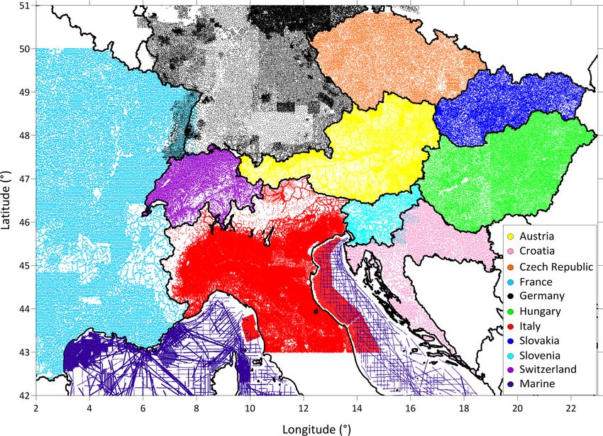
more significant errors in the transformed CBA. Figure 8                4     The new homogenized gravity maps for the Alps
shows a comparison of transformed CBA map with a map
constructed from available data within the project for Croa-            4.1    Interpolation and reference height of interpolated
tia. Fortunately, the differences between the maps are not sig-                Bouguer anomalies
nificantly large, the standard deviation of differences is about
1.8 mGal with a low systematic difference (the mean value of            AlpArray gravity data have different levels of confidentiality.
the differences is less than 0.5 mGal). We therefore assume             In some cases, only interpolated grids are available. There-
that the replaced anomaly in the southeastern part of the map           fore, well-defined interpolation procedures are required. In-
(Serbia, Bosnia and Herzegovina) is of similar quality than             terpolating scattered gravity data onto regular grids is com-
the main part.                                                          monly done in 2D, ignoring the fact that original data are ac-
                                                                        quired at different elevations rather than at a constant level.
                                                                        More exact solutions would be achieved by solving a proper
3.4    A short remark on future treatment of true                       boundary value problem. However, those methods are very
       atmosphere and distant relief effects                            time consuming, and avoiding mathematical artifacts due to
As a challenge for the further development of the AlpAr-                limitation of data in terms of spatial extent and resolution is
ray CBA map, we also estimated the global effects of the                not trivial at all. Hence, the AAGRG decided to provide grids
true atmosphere and distant relief. Atmospheric correction              based on 2D interpolation first.
is usually calculated based on a simple approximation ac-                  For assessing the 2D interpolation error in rugged ter-
cording to Wenzel (1985). By the term true atmosphere, we               rain, two synthetic gravity data sets have been created based
mean the model of the atmosphere derived from the effect                on two different kinds of source representation: a polyhe-
of a spherical shell with radially dependent density using              dron model (method by Götze and Lahmeyer, 1988) and an
the US standard atmosphere 1976 (Karcol, 2011) with an ir-              equivalent source model (EQS) determined by the method of
regularly shaped bottom surface formed by the Earth’s sur-              Cordell (1992). The model response has been calculated at
face, calculated globally (Mikuška et al., 2008). The dif-              the scattered positions of a subset of Austrian gravity data,
ference between atmospheric correction calculated by both               as well as at the grid nodes with 1 km spacing. The synthetic
approaches for the AlpArray region (calculated for selected             data sets almost keep the wavelength content of real-world
database points) is shown in Fig. 9. The differences reach a            data. The elevation at the grid nodes was interpolated by 2D-
maximum of about 0.16 mGal. As a function of height (ap-                Kriging based on the scattered data information.
prox. 0.04 mGal km−1 ) it mainly depends on the topography                 In the case of the polyhedron model, the differences be-
and to a much lesser extent also on the density model. Using            tween exact 3D prediction and 2D interpolation do not ex-
a linear approximation instead of a time-consuming calcu-               ceed the range of 1–2 mGal. Only in small, isolated areas
lation at specific points would lead to maximum errors of               are the errors larger than 5 mGal. The same holds for the
about 0.02 mGal. Note that in order to maintain the real sit-           equivalent source representation in which the errors are in
uation regarding the distribution of atmospheric masses, we             the range of ±1 mGal and exceed ±2 mGal only at a few
used physical heights, not ellipsoidal heights.                         spots (Fig. 11).
   Distant relief effect (DRE) represents the combined effect              In large-scale 3D modeling, 3D models rarely match the
of topography and bathymetry beyond a standard distance of              data better than the errors estimated in the scenarios tested
166.7 km around the whole Earth (refer to Mikuška et al.,               above. Therefore, 2D interpolation seems to be justified even
2006, for more detailed information). Figure 10 shows this              if it is not exact from a theoretical viewpoint. In local-scale
effect calculated at selected points in the AlpArray study              interpretation, the situation may be different. However, an-
area. The calculation was made in the classical concept                 other problem arises when using interpolated grids. Model-
of physical heights. The calculation for ellipsoidal heights            ers need to know the elevation to which interpolated Bouguer
would differ slightly (in quantitative terms), but the basic fea-       or free-air anomalies refer.
tures would be retained as presented. The inclusion of this ef-            Assuming the interpolation operator to be linear, Bouguer
fect in the CBA is a task for future studies. DRE is dominated          anomaly (BA) and free-air anomaly (FA) interpolated at each
mainly by long-wavelength trends, superimposing also high-              grid node (xi , yj ) read as
frequency patterns in mountainous regions due to its depen-
dence on height. Because terrain masses are largely compen-

Earth Syst. Sci. Data, 13, 2165–2209, 2021                                              https://doi.org/10.5194/essd-13-2165-2021
P. Zahorec et al.: The first pan-Alpine surface-gravity database                                                                                    2175

Figure 8. Comparison of CBA maps (density 2670 kg m−3 ) for the area of Croatia. The map on the left (a) is constructed from available
data within the AlpArray project. The map on the right (b) was obtained by transforming the digitized map of the former SFR Yugoslavia
(Bilibajkič et al., 1979). The histogram in the middle (c) shows the differences between the maps.

                                                                                 Figure 10. The summary effect of topography and bathymetry
Figure 9. Comparison of atmospheric correction at selected points                (densities of 2670 and −1640 kg m−3 , respectively) from 166.7 km
covering the whole AlpArray area. The black dots represent the at-               around the whole Earth.
mospheric correction calculated by a simple approximation accord-
ing to Wenzel (1985). The red dots show the calculation using the
effect of true atmosphere subtracted from the global constant value              respect to the reference ellipsoid. By transforming Eq. (7)
of 0.874 mGal (Mikuška et al., 2008), and the blue line is its linear            and using Eq. (8) we get
approximation.
                                                                                 FAint (xi , yj ) = BAint (xi , yj ) + MCint (xi , yj ).             (9)

                                                                                 Assuming the Bouguer anomaly to be a sufficiently smooth
                                                                                 function of horizontal coordinates, true gravity at the position
BAint (xi , yj ) = gint (xi , yj ) − γint (xi , yj ) − MCint (xi , yj ),   (7)   (xi , yj ) of a grid node and at the true elevation htopo (xi , yj )
FAint (xi , yj ) = gint (xi , yj ) − γint (xi , yj ),                      (8)   can be approximated by

where the suffix “int” denotes interpolated quantities and MC                    g(xi , yj , htopo ) ≈ grec (xi , yj , htopo ) = BAint (xi , yj )
is the gravitational effect of surplus and deficit mass with                        + γ (xi , yj , htopo ) + MC(xi , yj , htopo ),                  (10)

https://doi.org/10.5194/essd-13-2165-2021                                                          Earth Syst. Sci. Data, 13, 2165–2209, 2021
2176                                                                       P. Zahorec et al.: The first pan-Alpine surface-gravity database

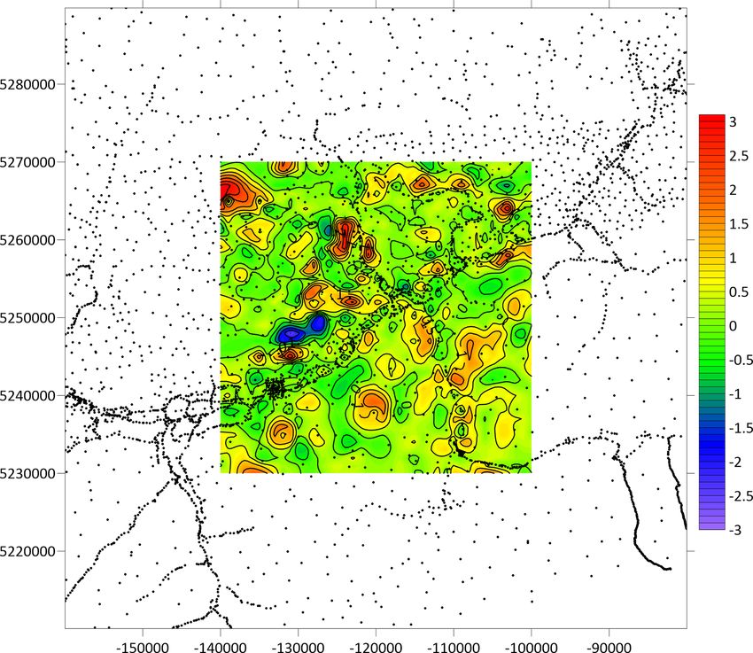
Figure 11. Interpolation error estimate (gravity difference between gravity fields predicted by the EQS model and by 2D interpolation;
contour interval 0.1 mGal, color bar in milligals (mGal) and axis coordinates in meters; Gauß–Krüger projection, M31).

where the suffix “rec” denotes approximated (reconstructed)                    being valid at the true elevation htopo (xi , yj ) of a grid node
quantities.                                                                    (xi , yj ) but also at elevation hint . Because interpolation is al-
  The Bouguer anomaly at grid node (xi , yj ) and at true el-                  ways associated with smoothing, we can argue that the best
evation htopo (xi , yj ) is                                                    location for referencing the Bouguer anomaly is hint . If mod-
                                                                               elers use true elevations for the grid nodes, then models based
BA(xi , yj , htopo ) = g(xi , yj , htopo ) − γ (xi , yj , htopo )              on polyhedron approaches suffer from an aliasing problem
     − MC(xi , yj , htopo ).                                        (11)       because the topography is not well represented by the grid.
                                                                               A smoothed (interpolated) topography would work better be-
Approximating g(xi , yj , htopo ) by Eq. (10) and inserting it                 cause interpolation includes a kind of filtering.
into Eq. (11) results in                                                          Particularly in rugged terrain, FA and MC are not smooth
                                                                               functions of horizontal coordinates. Therefore, applying Eq.
BA(xi , yj , htopo ) ≈ BAint (xi , yj ) + γ (xi , yj , htopo )                 (9) is rather questionable. Instead, the free-air anomaly at a
     + MC(xi , yj , htopo ) − γ (xi , yj , htopo )                             grid node (xi , yj ) and at true elevation htopo (xi , yj ) can be
     − MC(xi , yj , htopo )                                                    better approximated by

or                                                                             FA(xi , yj , htopo ) ≈ FArec (xi , yj , htopo )
BA(xi , yj , htopo ) ≈ BAint (xi , yj ).                            (12)          = grec (xi , yj , htopo ) − γ (xi , yj , htopo )
                                                                                  = BAint (xi , yj ) + MC(xi , yj , htopo ).                  (13)
However, this approach neglects the fact that the Bouguer
anomaly is the gravity effect of all sources at the true loca-
                                                                               Inserting Eq. (7) into Eq. (13) results in
tion of a station and therefore depends on the station heights
as well. We would get the same result as in Eq. (12) for any
arbitrary elevation h used in Eqs. (10) to (12), also for hint .               FA(xi , yj , htopo ) ≈ gint (xi , yj ), −γint (xi , yj )
Hence, we can interpret the interpolated Bouguer anomaly as                       − MCint (xi , yj ) + MC(xi , yj , htopo )

Earth Syst. Sci. Data, 13, 2165–2209, 2021                                                        https://doi.org/10.5194/essd-13-2165-2021
P. Zahorec et al.: The first pan-Alpine surface-gravity database                                                                2177

or with Eq. (8)                                                     Toulouse (Förste et al., 2014) and EGM2008 (Pavlis et al.,
                                                                    2012). Both models are created by the combination of satel-
FA(xi , yj , htopo ) ≈ FAint (xi , yj ) − MCint (xi , yj )          lite and terrestrial gravity data. The spatial resolution of these
   + MC(xi , yj , htopo ).                                   (14)   models is roughly about 10 km.
                                                                       The GGMs are usually used in connection with the so-
The free-air anomaly at the true elevation htopo (xi , yj ) of a    called residual terrain modeling (RTM) technique, which
grid node (xi , yj ) can be reconstructed either by Eq. (13) or     greatly improves gravity values calculated from GGMs on
(14). However, also in this case we have to keep in mind            the Earth’s surface. The RTM technique accounts for the dif-
that we actually do not overcome the problem of the height          ference between the gravitational effect of the real terrain
dependence of Bouguer anomalies. When we use hint instead           masses represented by high-resolution DEMs and smoothed
of htopo , Eqs. (13) and (14) hold accordingly.                     mean elevation surface represented, e.g., by the DTM2006
   Note that we implicitly also included bathymetry in the          model (Pavlis et al., 2007). However, since the effect of
MC term appearing in Eqs. (7) to (14). Regarding the                the detailed DEM would be subtracted retrospectively in the
Bouguer anomaly BAρ calculated with density ρ differing             Bouguer anomaly calculation, it means that, in order to ob-
from density ρ0 used in the mass correction (MC) term in            tain BA, we only need to subtract the gravity effect of the
Eqs. (7) to (14), we have to separate liquid from solid parts,      DTM2006 (δgDTM2006 (λ, ϕ, hE )) directly from the free-air
which leads to the following equation:                              anomaly calculated from GGM-derived gravity by the stan-
                                   
                                           ρ
                                                                   dard procedure of Eq. (16). Compared to Eq. (1), Eq. (16)
BAρ (xi , yj ) = BAint (xi , yj ) + 1 −                             lacks the term for the atmospheric correction because it is
                                          ρ0
                                                                  already included in the GGM:
                        ρ − ρoc
   δgM (xi , yj ) 1 −                δgB (xi , yj ),        (15)
                        ρ0 − ρoc                                    BAGGM (λ, ϕ, hE ) =gGGM (λ, ϕ, hE ) − γ (ϕ, hE )
                                                                                          − δgDTM2006 (λ, ϕ, hE ),               (16)
where ρoc is the density of ocean water (1030 kg m−3 ).
   Equation (15) neglects the small density difference be-          where gGGM is the gravity calculated from a particular
tween lake and ocean water. However, this leads to only small       GGM at the Earth’s surface (to be directly comparable with
errors on the order of a few percent of the lake correction for     the terrestrial data) at elevations derived from the MERIT
reasonable crustal densities.                                       model, γ is the normal gravity, and δgDTM2006 is the gravita-
   To conclude, in addition to the methodological procedures        tional (terrain and bathymetry) effect related to the model
just described, we will now describe another problem related        DTM2006 (of the corresponding degree of 2190) up to
to the gridding of our database. In the case of the AAGRG           the distance of 166.7 km. The DTM2006 model was se-
compilation, interpolation of original and gridded data has         lected due to its close relationship with the creation of the
been done by an iterative procedure:                                model EGM2008. This model was originally compiled in a
  a. Data providers, who were not allowed to release orig-          grid of 30 arcsec × 30 arcsec. For the purposes of our cal-
     inal information, created gridded data relying initially       culations, the model was transformed and resampled into
     on their own scattered data and keeping only the nodes         a format corresponding to the calculation of the standard
     inside their own territory on a grid the AAGRG defined         mass/bathymetric correction using Toposk.
     in common for the whole area.                                     We calculated the gravity values gGGM using the software
                                                                    GrafLab (Bucha and Janák, 2013) using the maximum de-
  b. After merging all data sets from AAGRG members one             gree of spherical harmonic coefficients for a specific GGM.
     common grid was interpolated.                                  Calculations were performed in GRS80 ellipsoidal coordi-
                                                                    nates.
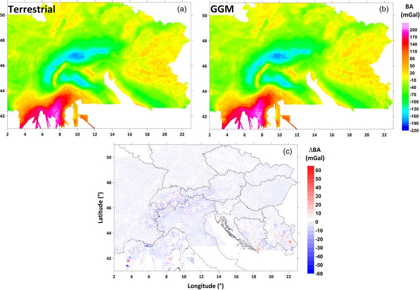
  c. In the next step grid nodes of the neighboring countries          Figure 12 shows a comparison of a BA map derived from
     were merged with the provider’s original data set, and a       terrestrial data with the map derived from the EIGEN-6C4
     new data grid was interpolated.                                model (calculation points were made on a 2 km × 2 km grid)
  d. This iterative procedure continued until the variation of      in the area covered by terrestrial data. The maximum differ-
     interpolated grid data close to the borders was well be-       ences between grids are at the level of tens of milligals (RMS
     low an error threshold defined by ±1.5 mGal.                   error is about 4 mGal) but without any systematic error. It
                                                                    follows that the GGM-derived map can be used to fill in gaps
                                                                    (marginal parts) in the terrestrial data.
4.2   Filling data gaps using global geopotential models
                                                                       GGM data points located in gaps of the original grav-
      (GGMs)
                                                                    ity points were separated by the shortest distance criteria of
We have focused on commonly used global geopotential                15 km using a standard database search query in QGIS. A
models (GGMs) up to the degree/order of 2190, mainly on             15 km criterion was chosen as a compromise between cover-
EIGEN-6C4 elaborated jointly by GFZ Potsdam and GRGS                ing GGM data close enough to the vicinity of the terrestrial

https://doi.org/10.5194/essd-13-2165-2021                                           Earth Syst. Sci. Data, 13, 2165–2209, 2021
2178                                                              P. Zahorec et al.: The first pan-Alpine surface-gravity database

Figure 12. Comparison of Bouguer anomaly maps (correction density 2670 kg m−3 ) derived from terrestrial data (a) and GGM EIGEN-
6C4 (b). The bottom map (c) shows the difference between the two.

data (Fig. 19) but at the same time not filling gaps that are         with the Northern Apennine gravity low. In the southeast-
too small between them, which could lead to local artificial          ernmost part of the Central Apennines the CAGL thins out
anomalies.                                                            gradually.
                                                                         A significant anomaly feature represented by a very nar-
                                                                      row local gravity high can be clearly recognized between the
4.3    Brief interpretation of Bouguer anomaly map                    Western Alps and the Po Basin. This anomaly is well known
                                                                      as the Ivrea gravity high (IGH). It is characterized by max-
We here present a short overview of the features of the new
                                                                      imum values of +40 mGal caused by dense, lower crustal
Bouguer anomaly map (Fig. 13). The most prominent fea-
                                                                      and mantle rocks that are exposed and in the near subsurface
ture of the complete Bouguer anomaly (CBA) is the Alpine
                                                                      and that are planned to be drilled in the forthcoming DIVE
gravity low (AGL), which is characterized by gravity values
                                                                      project (Pistone et al., 2017; http://dive.icdp-online.org/, last
ranging from −100 to −170 mGal. The AGL corresponds
                                                                      access: 15 May 2021). It is important to note that its relative
with the Alpine mountain chain and is explained by the iso-
                                                                      amplitude compared to the gravity lows in the Western Alps
static crustal thickening, as demonstrated by the good anti-
                                                                      and the Po Basin reaches up to 160 mGal. It is the highest
correlation with topography (Braitenberg et al., 2013; Pivetta
                                                                      horizontal gravity gradient in the study region.
and Braitenberg, 2020) and the isostatic compensation and
                                                                         To the northeast of the Po Basin, we can observe the
gravity forward models (e.g., Ebbing et al., 2006; Braiten-
                                                                      Verona/Vicenza gravity high (VVGH), which has been re-
berg et al., 2002). It could be divided into local gravity lows
                                                                      cently modeled as being generated by increased density
that correlate with the Western, Central and Eastern Alps.
                                                                      crustal intrusions related to the Venetian magmatic province
Among all of them the Central Alps (the easternmost part
                                                                      (Tadiello and Braitenberg, 2021; Ebbing et al., 2006). The
of Switzerland) are accompanied by the highest amplitude:
                                                                      Venetian/Friuli Plain gravity low (VFGL) is located in east-
−170 mGal.
                                                                      ern Italy, which is presumably caused by low-density sedi-
   A second prominent low is the Po Basin gravity low
                                                                      mentary infill, also like the gravity low in the Po Basin (Brait-
(PoBGL). The gravity values here range from about −80 to
                                                                      enberg et al., 2013).
−140 mGal. The PoBGL continues in the southeastern di-
                                                                         A prominent gravity high is the Mediterranean gravity
rection to the Central Apennine gravity low (CAGL), whose
                                                                      high (MGHi). This regional-scale anomaly has its maximum
amplitude (−40 mGal) is significantly smaller in comparison

Earth Syst. Sci. Data, 13, 2165–2209, 2021                                            https://doi.org/10.5194/essd-13-2165-2021
P. Zahorec et al.: The first pan-Alpine surface-gravity database                                                               2179

Figure 13. New pan-Alpine Bouguer gravity anomaly map. The first order dominant regional gravity anomalies: AGL – Alpine gravity low,
PoBGL – Po Basin gravity low, CAGL – the Central Apennine gravity low, IGH – Ivrea gravity high, VVGH – Verona/Vicenza gravity high,
VFGL – Venetian/Friuli Plain gravity low. The second dominant regional gravity anomaly: MGHi – Mediterranean gravity high, CLGH –
Corso/Ligurian gravity high, TGH – Tyrrhenian gravity high, CSGL – Corsica/Sardinia gravity low, SAGH – south Adriatic gravity high,
IGH – Istria gravity high, WCGL – Western Carpathian gravity low, DGL – Dinaric gravity low, MeGH – Merdita gravity high, ADGL –
pre-Adriatic depression, PBGH – Pannonian Basin gravity high, TDGH – Transdanubian gravity high, PGH – Papuk gravity high, MsGH
– Mecsek gravity high, FGGH – Fruška Gora gravity high, DBGL – Danube Basin gravity low, MBGL – Makó/Békés Basin gravity low,
APGL – Apuseni gravity low. The rest of the study area: PGL – Pyrenean gravity low, MCGL – Massif Central gravity low, PBGL – Paris
Basin gravity low, URGGL – Upper Rhine graben gravity low, RBGH – Rhône/Bresse Graben gravity high, BFGH – Black Forest gravity
high, VGH – Vosgesian gravity high, KKGL – Krušné hory (Erzgebirge)/Krkonoše gravity low, TBLGH – Tepla/Barrandian/Labe gravity
high, MGL – Moldanubic gravity low, OOGL – Orlice/Opole gravity low, MSGH – Moravo/Silesian gravity high, USGH – Upper Silesian
gravity high, SGH – Sudetes gravity high, KB – Krško Basin. A high resolution 600 dpi plot of the map is available in the supplement.

over the Corso/Ligurian Basin, the Corso/Ligurian gravity            ern Carpathian gravity low (WCGL) and the Dinaric grav-
high (CLGH). It is characterized by maximum values of                ity low (DGL). In the Western Carpathians, the values vary
+200 mGal. The regional MGHi also includes the Tyrrhe-               from 0 to −60 mGal, while the Dinaric values range from 0
nian gravity high (TGH). The study covers only the north-            to −120 mGal (Bielik et al., 2006). The lower amplitude of
ern part. Gravity values do not exceed +140 mGal. The                the gravity field of both the WCGL and the DGL in compar-
Corso/Ligurian gravity high and the Tyrrhenian gravity high          ison with the AGL most likely reflects a weaker continental
are separated from the relative Corsica/Sardinia gravity low         collision resulting in thinner crust under the Carpathians and
(CSGL). The values vary from +20 to +60 mGal.                        Dinarides. In the Adriatic region we can also recognize the
   The Adriatic Sea region is largely characterized by a pos-        Merdita gravity high (MeGH) and the pre-Adriatic gravity
itive gravity field, in which the south Adriatic gravity high        low (ADGL).
(SAGH) dominates with values from +20 to +100 mGal. Its                 The Pannonian Basin extending between the Western
maximum is located over the Gargano promontory. In the               Carpathians and the Dinarides is accompanied by a rela-
northwestern part of the Adriatic Sea, negative gravity val-         tively regional gravity high (Pannonian Basin gravity high,
ues up to −80 mGal are observed, which belong to the east-           PBGH) whose values range in a narrow interval from −10
ernmost part of the Po Basin gravity low. West of the Istrian        to +20 mGal. The PBGH consists of several local positive
peninsula the center of the residual Istria gravity high (IGH)       (the Transdanubian gravity high, TDGH, the Papuk gravity
is present, with maximum values of +30 mGal.                         high, PGH, the Mecsek gravity high, MsGH, the Fruška Gora
   In the Eastern Alps, the AGL splits towards the east into         gravity high, FGGH) and negative anomalies (the Danube
two branches of less pronounced gravity lows: the West-              Basin gravity low, DBGL, the Makó-Békés Basin gravity

https://doi.org/10.5194/essd-13-2165-2021                                           Earth Syst. Sci. Data, 13, 2165–2209, 2021
You can also read