The INFRA-EAR: a low-cost mobile multidisciplinary measurement platform for monitoring geophysical parameters
←
→
Page content transcription
If your browser does not render page correctly, please read the page content below
Atmos. Meas. Tech., 14, 3301–3317, 2021
https://doi.org/10.5194/amt-14-3301-2021
© Author(s) 2021. This work is distributed under
the Creative Commons Attribution 4.0 License.

The INFRA-EAR: a low-cost mobile multidisciplinary measurement
platform for monitoring geophysical parameters
Olivier F. C. den Ouden1,2 , Jelle D. Assink1 , Cornelis D. Oudshoorn3 , Dominique Filippi4 , and Läslo G. Evers1,2
1 R&D  Department of Seismology and Acoustics, Royal Netherlands Meteorological Institute, De Bilt, the Netherlands
2 Dept.of Geoscience and Engineering, Delft University of Technology, Delft, the Netherlands
3 R&D Department of Observations and Data Technology, Royal Netherlands Meteorological Institute,

De Bilt, the Netherlands
4 Sextant Technology, Inc., Marton, New Zealand

Correspondence: Olivier F. C. den Ouden (olivier.den.ouden@knmi.nl)

Received: 11 September 2020 – Discussion started: 2 December 2020
Revised: 16 February 2021 – Accepted: 31 March 2021 – Published: 4 May 2021

Abstract. Geophysical studies and real-time monitoring of        is used to protect the mobile platform against the weather.
natural hazards, such as volcanic eruptions or severe weather    The casing is created with a stereolithography (SLA) Form-
events, benefit from the joint analysis of multiple geophys-     labs 3D printer using durable resin.
ical parameters. However, typical geophysical measurement           Thanks to low power consumption (9 Wh over 25 d), the
platforms still provide logging solutions for a single parame-   system can be powered by a battery or solar panel. Besides
ter, due to different community standards and the higher cost    the description of the platform design, we discuss the cali-
per added sensor.                                                bration and performance of the individual sensors.
   In this work, the Infrasound and Environmental Atmo-
spheric data Recorder (INFRA-EAR) is presented, which has
been designed as a low-cost mobile multidisciplinary mea-
surement platform for geophysical monitoring. In particular,     1   Introduction
the platform monitors infrasound but concurrently measures
barometric pressure, accelerations, and wind flow and uses       Real-time monitoring of natural hazards, such as volcanic
the Global Positioning System (GPS) to position the plat-        eruptions or severe weather events benefit from the joint anal-
form. Due to its digital design, the sensor platform can be      ysis of multiple geophysical parameters. However, geophysi-
readily integrated with existing geophysical data infrastruc-    cal measurement platforms are typically designed to measure
tures and be embedded in geophysical data analysis. The          a single parameter, due to different community standards and
small dimensions and low cost per unit allow for unconven-       the higher cost per added sensor. The quality and robustness
tional, experimental designs, for example, high-density spa-     of geophysical measuring equipment generally scale with
tial sampling or deployment on moving measurement plat-          price, due to higher material costs and research and develop-
forms. Moreover, such deployments can complement ex-             ment (R&D) expenses. In addition, the deployment of such
isting high-fidelity geophysical sensor networks. The plat-      equipment comes with complex deployment and calibration
form is designed using digital micro-electromechanical sys-      procedures and requires the presence of a robust power and
tem (MEMS) sensors embedded on a printed circuit board           data infrastructure.
(PCB). The MEMS sensors on the PCB are a GPS, a                     Geophysical institutes often place multiple sensor plat-
three-component accelerometer, a barometric pressure sen-        forms co-located. Meteorological institutes, for example,
sor, an anemometer, and a differential pressure sensor. A pro-   measure various meteorological parameters for comparison,
grammable microcontroller unit controls the sampling fre-        which improves the weather observations and weather fore-
quency of the sensors and data storage. A waterproof casing      cast models. The Comprehensive Nuclear-Test-Ban Treaty
                                                                 Organization (CTBTO) performs various geophysical mea-

Published by Copernicus Publications on behalf of the European Geosciences Union.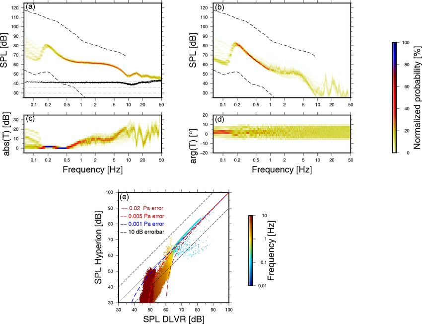
3302                                                                             O. F. C. den Ouden et al.: The INFRA-EAR

surements at its measurement sites where possible. The In-            In this work, the INFRA-EAR is presented, which has
ternational Monitoring System (IMS), which is in place for         been designed as a low-cost mobile multidisciplinary mea-
verification of the Comprehensive Nuclear Test Ban Treaty          surement platform for geophysical monitoring, in particular,
(CTBT), performs continuous seismic, hydroacoustic, infra-         infrasound. The platform uses various digital MEMS sensors
sonic, and radionuclide measurements (Marty, 2019). In ad-         embedded on a printed circuit board (PCB). A programmable
dition, the IMS infrasound arrays and radionuclide facilities      microcontroller unit, as well embedded on the PCB, con-
host auxiliary meteorological equipment, as this data facil-       trols the sensors’ sampling frequency and establishes the en-
itates the review of the primary IMS data streams. Besides         ergy supply for the sensors and the data communication and
its use for verifying the CTBT, it has also been shown that        storage. A waterproof casing protects the mobile platform
a multi-instrumental observation network such as the IMS           against the weather. The casing is created with a stereolithog-
can provide useful information on the vertical dynamic struc-      raphy (SLA) Formlabs 3D printer using durable resin. Be-
ture of the middle and upper atmosphere, in particular when        cause of its low power consumption, the system can be pow-
paired with complementary upper atmospheric remote sens-           ered by a battery or solar panel.
ing techniques such as lidar (Blanc et al., 2018). Other stud-        Previous studies have presented similar mobile infrasound
ies that involve the analysis of multiple geophysical parame-      sensor designs (Anderson et al., 2018; Marcillo et al., 2012;
ters include seismo-acoustic analyses of explosions (Assink        RBOOM, 2017), which have shown how low-cost, minia-
et al., 2018; Averbuch et al., 2020), earthquakes (Shani-          ture sensors can complement existing measurement network
Kadmiel et al., 2018), and volcanoes (Green et al., 2012).         (e.g., volcanic and earthquake monitoring). Those platforms
   National weather services, such as the Royal Netherlands        differ from the INFRA-EAR in dimension, multidisciplinary
Meteorological Institute (KNMI), have expressed an inter-          purpose, and digital design. All sensors of the INFRA-EAR
est in measuring weather on a local scale to inform and            have a built-in analogue-to-digital converter (ADC), which
warn citizens of extreme weather. In addition, such mea-           directly generates digital outputs. Therefore, the INFRA-
surements allow for higher-resolution measurements of sub-         EAR can be easily integrated into the existing hardware and
grid scale atmospheric dynamics, which will contribute to          software sensor infrastructure. Furthermore, the casing de-
the improvement of short-term and nowcasting weather fore-         sign and development is based on the latest technology of
casts (Manobianco and Short, 2001; Lammel, 2015). There-           3D printing. Furthermore, the platform design and purpose
fore it became part of a low-cost citizen weather station pro-     are adaptive to various monitoring campaigns.
gram to increase the spatial resolution of conventional nu-           The ability to detect infrasonic signals of interest depends
merical weather prediction models. In the Netherlands, over        on the signal’s strength relative to the noise levels at the
300 of those weather stations contribute to a global citi-         receiver side, the signal-to-noise ratio (SNR). The signal
zen science project, Weather Observations Website (WOW)            strength depends on the transmission loss that a signal ex-
(Garcia-Marti et al., 2019; Cornes et al., 2020). Nonetheless,     periences propagating from source to receiver. Infrasound
due to the required infrastructure of the equipment, many          measurements benefit from insights in the atmospheric noise
platforms are spatially static. Having a low-cost multidis-        levels (e.g., wind conditions), the meteorological conditions
ciplinary mobile sensor platform allows for high-resolution        (e.g., barometric pressure, temperature, and humidity), as
spatial sampling and complements existing high-fidelity geo-       well as the movement and positioning of the sensors (e.g.,
physical sensor networks (e.g., buoys in the open ocean,           accelerations) (Evers, 2008).
Grimmett et al., 2019; and stratospheric balloons, Poler et al.,      While there are clear benefits associated with a MEMS-
2020).                                                             based mobile platform (e.g., cheap and rapid deployments to
   Various disciplines apply new sensor technology to ob-          (temporarily) increase coverage), MEMS sensors are known
tain higher spatial and temporal resolution (D’Alessandro          to be less accurate than conventional high-fidelity equipment.
et al., 2014) for geophysical hazard monitoring. Micro-            Digital MEMS sensors, which have a built-in ADC, are espe-
electromechanical systems (MEMS) are small single-chip             cially known for their high self-noise level. Nonetheless, they
sensors that combine electrical and mechanical components          could be used near geophysical sources that generate high
and have low energy consumption. The seismic community             SNR. Several geophysical measurements (Marcillo et al.,
has created low-cost reliable MEMS accelerometers (Home-           2012; Grangeon and Lesage, 2019; Laine and Mougenot,
ijer et al., 2011; Milligan et al., 2011; Zou et al., 2014) to     2007; D’Alessandro et al., 2014) show the benefit of MEMS
detect strong accelerations that exceed values due to Earth’s      sensors and how they complement the existing sensor net-
gravity field (Speller and Yu, 2004; Laine and Mougenot,           work.
2007; Homeijer et al., 2014). Moreover, the infrasound (Mar-          In this paper, the design and calibration of the INFRA-
cillo et al., 2012; Anderson et al., 2018) and meteorological      EAR is discussed. Due to its digital design, the platform can
community are integrating MEMS sensors into the existing           readily be integrated into existing geophysical sensor infras-
sensor network (Huang et al., 2003; Fang et al., 2010; Ma          tructures. The remainder of this article is organized as fol-
et al., 2011).                                                     lows. Section 2 introduces the mobile platform, its design,
                                                                   and its features. Section 3 describes the various sensors em-

Atmos. Meas. Tech., 14, 3301–3317, 2021                                             https://doi.org/10.5194/amt-14-3301-2021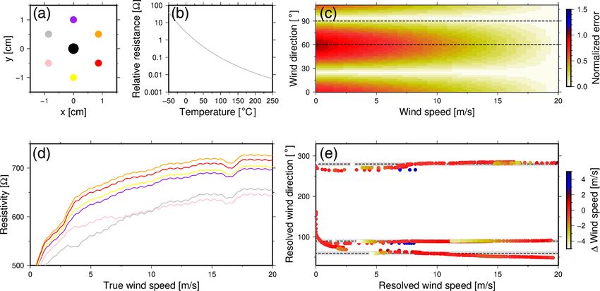
O. F. C. den Ouden et al.: The INFRA-EAR                                                                                     3303

bedded on the platform and the relative calibrations with         casing is waterproof and airtight. At the bottom of the casing,
high-fidelity reference equipment. Firstly, a novel miniature     a dome structure is integrated (Fig. 1c), which acts as an in-
digital infrasound sensor is introduced and its theoretical re-   let to both the absolute and differential pressure sensors. Note
sponse is derived. Secondly, the barometric MEMS sensor is        that the dome is not connected to the inside of the casing. The
discussed. A wind sensor that relies on thermo-resistive ele-     inlets of both sensors and a capillary are integrated within the
ments is discussed next, followed by a discussion of the on-      dome designs and sealed with silicone glue, avoiding water
board MEMS accelerometer. In Sect. 4, the platform’s overall      and air leakage. Moreover, a Gore-Tex air-vent sticker (Gore-
performance and design are discussed and summarized, from         Tex, 2020) is used to cover the dome, which allows airflow
which the conclusions are drawn.                                  but restrains water and salt in measurements near or above
                                                                  the ocean.
                                                                     Air turbulence can generate dynamic pressure effects or
2     Mobile platform design                                      stagnation pressure at the pressure dome (Raspet et al.,
                                                                  2019). The stagnation pressure increases with altitude, which
2.1    Circuit design
                                                                  results in higher wind speeds. Atmospheric measurements at
The mobile platform contains a PCB created to embed the           altitude might therefore be influenced by stagnation pressure
MEMS sensors and facilitate the electrical circuits. The PCB      (Bowman and Lees, 2015; Smink et al., 2019; Krishnamoor-
carries a digital low voltage range (DLVR) differential pres-     thy et al., 2020). The influence of stagnation pressure on
sure sensor, an anemometer, as well as an accelerometer and       pressure measurements is theoretically elucidated by Raspet
barometric pressure sensor in addition to a GPS for location      et al. (2008).
and timing purposes (Fig. 1a). The sensors are controlled by         The application of a quad-disk might remove the stag-
a MSP430 microcontroller, which is integrated on the PCB,         nation pressure. Quad-disks are developed to cancel dy-
and are powered by an 1800 mAh lithium battery. Protect-          namic pressure effects and help detect slower static pressure
ing the PCB is done with a weather- and waterproof cas-           changes or acoustic perturbations. Theoretical analysis of the
ing, which has been designed (Fig. 1b) with the dimensions        quad-disk indicates that it should remove sufficient dynamic
110 mm × 38 mm × 15 mm.                                           pressure to be useful for turbulence studies (Wyngaard and
   The communication between the microcontroller and              Kosovic, 1994). However, recent studies have shown a min-
MEMS sensor on the PCB is either done by inter-integrated         imum effect of quad-disks on infrasound recordings (Krish-
circuit (I2C) or serial peripheral interface (SPI) and depends    namoorthy et al., 2020). The casing of the INFRA-EAR is
on the sensor and personal preference. Both communication         designed and developed for mobile and rapid deployments at
methods are bus protocols and allow for serial data trans-        remote places; adding a quad-disk to the design will expand
fer. However, SPI handles full-duplex communication, si-          the dimensions of the casing. Moreover, the pressure dome is
multaneous communication between the microcontroller and          positioned at the bottom of the casing, not oriented towards
MEMS sensor, while I2C is half-duplex. Therefore, I2C has         the dominant wind direction, in order to minimize the stag-
the option of clock stretching, and the communication is          nation pressure on the pressure sensors.
stopped whenever the MEMS sensor cannot send data. In                Furthermore, within this design, the casings volume acts
addition, I2C has built-in features to verify the data commu-     as a backing volume for the differential pressure sensor. One
nication (e.g., start/stop bit, acknowledgement of data). Al-     inlet of the differential pressure sensor is attached to the out-
though the I2C protocol is favorable, it requires more power.     side (via the dome) while the casing encloses the other inlet.
   The microcontroller runs on self-made software, comple-        A PEEKsil red series capillary is attached to the outside of
menting the required manufacturers electrical and communi-        the casing, ensuring pressure leakage between the backing
cation protocols. The software allows one to determine the        volume and the atmosphere.
sample time, sample frequency, and data storage. The PCB
                                                                  2.3   GPS
includes a 64 MB flash memory, which is used to store the
data. The raw output of the digital MEMS sensors are stored       For measuring geophysical parameters on a high-resolution
as bits and the microcontroller performs no data process-         temporal scale, it is crucial to know the position and time of
ing to save power consumption. To extract data, the platform      the measurement at high precision. To maintain knowledge
needs to be connected to a computer. There are no wireless        regarding the position, a GNS2301 GPS is mounted on the
communication possibilities.                                      PCB (Texim Europe, 2013). The GPS has a spatial accuracy
                                                                  of ±2.5 m up to 20 km altitude.
2.2    Casing design for pressure measurements
                                                                     Besides providing an accurate position, the GPS also pre-
The mobile sensor platform is designed to measure atmo-           vents drifting of the microcontroller’s internal clock under
spheric parameters. Hence, a waterproof casing has been cre-      the influence of, for example, weather. The time root mean
ated using a Formlabs SLA 3D printer (Formlabs, 2020) to          square jitter, the deviation between GPS and actual time, is
protect the PCB. Because of the use of a durable resin, the       ±30 ns.

https://doi.org/10.5194/amt-14-3301-2021                                            Atmos. Meas. Tech., 14, 3301–3317, 2021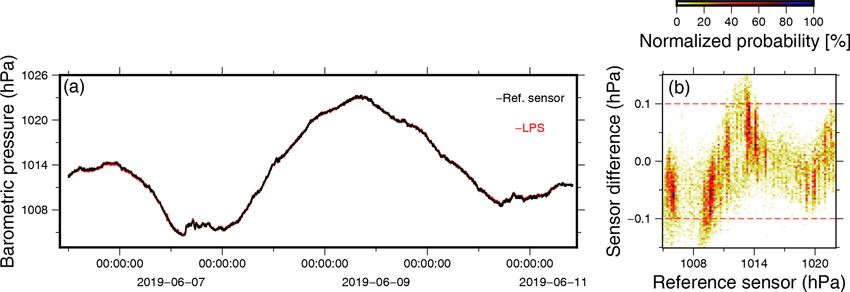
3304 O. F. C. den Ouden et al.: The INFRA-EAR
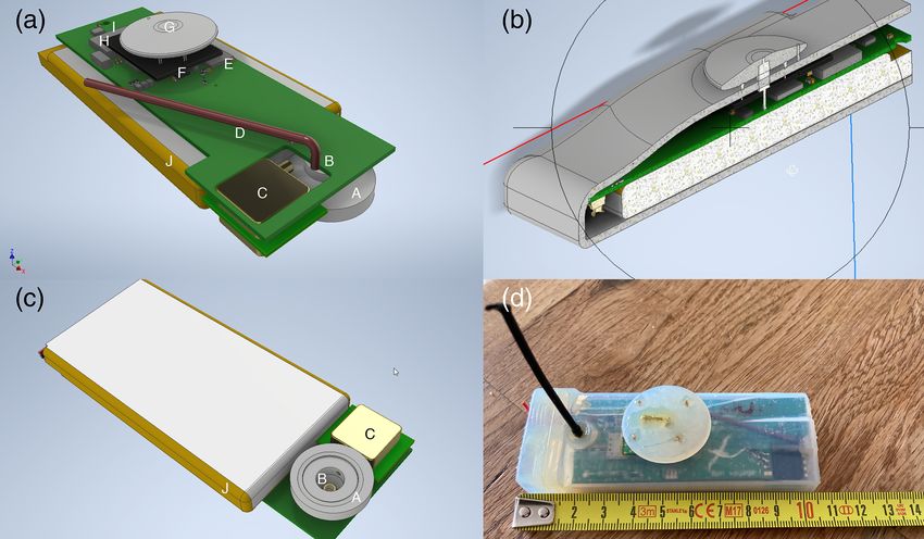
Figure 1. 3D CAD design of (a) the top of the PCB, (b) the casing, (c) the bottom of the PCB with pressure dome, and (d) a picture of the
actual platform. The PCB hosts: a pressure dome (a-A/c-A), a barometric pressure sensor (a-B/c-B), a differential pressure sensor (a-C/c-C),
a PEEKsil red series capillary (a-D), an accelerometer (a-F), an anemometer (a-F) with the heating element (a-G), a microcontroller (a-H), a
GPS (a-I), and a lithium battery (a-J/c-J).
3 Sensor descriptions absolute pressure sensor consists of a sealed aneroid and
a measuring cavity connected to the atmosphere. A pres-
3.1 Infrasound sensor sure difference within the measuring cavity will deflect the
aneroid capsule. The mechanical deflection is converted to a
voltage (Haak and De Wilde, 1996). The measurement prin-
The human audible sound spectrum is approximately be-
ciple of a differential infrasound sensor relies on the deflec-
tween 20 and 20 000 Hz. Frequencies below 20 Hz or above
tion of a compliant diaphragm, which is mounted on a cav-
20 kHz are referred to as infrasound and ultrasound, respec-
ity inside the sensor. The membrane deflects due to a pres-
tively. The movement of large air volumes generates infra-
sure difference inside and outside the microphone, which oc-
sound signals with amplitudes in the range of millipascals
curs when a sound wave passes. A pressure equalization vent
to tens of pascals. Examples of infrasound sources include
is part of the design to make the microphone insensitive to
earthquakes, lightning, meteors, nuclear explosions, interfer-
slowly varying pressure differences originating from long-
ing oceanic waves, and surf (Campus and Christie, 2010).
period changes in weather conditions (Ponceau and Bosca,
Detection of infrasound depends on the signal’s strength rel-
2010).
ative to the noise levels at a remote sensor (array), i.e., the
Acoustic particle velocity sensors constitute a fundamen-
signal-to-noise ratio. The signal strength depends, in turn, on
tally different class of sensors that measure the airflow over
the transmission loss that a signal experiences while propa-
sets of heated wires. This information quantifies the 3D par-
gating from source to receiver (Waxler and Assink, 2019).
ticle velocity at one location, since the measurement is car-
Local wind noise conditions predominantly determine the
ried out in three directions (De Bree, 2003; Evers and Haak,
noise (Raspet et al., 2019) in addition to the sensor self-noise.
2000). Although such sensors’ design is more involved and
Due to the presence of atmospheric waveguides and low ab-
the sensors are far more costly, these sensors do allow for
sorption at infrasonic frequency (Sutherland and Bass, 2004),
the measurement of sound directivity at one position, besides
infrasonic signals can be detected at long distances from an
just the loudness.
infrasonic source. It is assumed that the source levels are suf-
Various studies show sensor self-noise and sensitivity
ficiently high so that the long-range signal is above the am-
curves of infrasound sensors (Ponceau and Bosca, 2010;
bient noise conditions on the receiver side and the sensor is
Merchant, 2015; Slad and Merchant, 2016; Marty, 2019;
sensitive enough to detect the signal.
Nief et al., 2019). The IMS specifications state that the sensor
The infrasonic wavefield is conventionally measured with
self-noise should be at least 18 dB below the global low-noise
pressure transducers since such scalar measurements are rel-
curves at 1 Hz (Brown et al., 2014), generated from global
atively easy to perform. Those measurements can either be
infrasound measurements using the IMS. Typical infrasound
performed by absolute or differential pressure sensors. An
Atmos. Meas. Tech., 14, 3301–3317, 2021 https://doi.org/10.5194/amt-14-3301-2021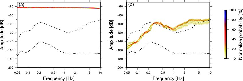
O. F. C. den Ouden et al.: The INFRA-EAR                                                                                         3305

sensor networks, such as the IMS, use analogue sensors con-           A theoretical response D(iω) for a differential pressure
nected to a separate data logger to convert the measured volt-     sensor as function of the angular frequency ω(= 2πf ) has
age differences to a digital signal. The sensor’s characteristic   been derived by Mentink and Evers (2011) following Bur-
sensitivity determines the sensor resolution, i.e., the smallest   ridge (1971):
difference that the sensor can detect. The resolution of the
built-in analogue-to-digital (ADC) converters and the digi-                              iωτ2
                                                                   D(iω) =                                ,                       (1)
tizing voltage range determine the data logger’s resolution.                   1 + iωτ2 A + (iω)2 τ1 τ2 B
Current state-of-the-art data loggers have a 24-bit resolu-
                                                                   where
tion. New infrasound sensor techniques involve digital out-

puts since the ADC conversion is realized inside the sensor                 τ1 R1 Cd                   1   1
(Nief et al., 2017, 2019).                                         A = 1+ +        +    , B = 1 + Cd     +                        (2)
                                                                            τ2 R2 C2                   C1 C2
                                                                                      Vj
3.1.1   Sensor design                                              τj = Rj Cj , Cj =        ,                                     (3)
                                                                                     Patm γ
In this section, the mobile digital infrasound sensor’s design
                                                                   Patm indicates the ambient barometric pressure, and γ is the
is discussed, the KNMI mini-microbarometer (mini-MB).
                                                                   thermal conduction of air. τj represent the time constants and
The design of this instrument is based on the following re-
                                                                   depend on R1 and R2 , which are the resistances of the inlet
quirements. The sensor should have a flat, linear response
                                                                   and capillary, and C1 and C2 , the capacities of the fore and
over a wide infrasonic frequency band, e.g., 0.05–10 Hz. The
                                                                   backing volume.
sensor should be sensitive to the range of pressure perturba-
                                                                      Figure 2a represents the sensor setup from an acousti-
tions in this frequency band, which are in the range of milli-
                                                                   cal perspective, where Fig. 2b represents the electrical ana-
pascals to tens of pascals. Moreover, the sensor and logging
                                                                   logues of the sensor. The acoustical pressure difference (p 0 =
components’ self-noise should be below the ambient noise
                                                                   p10 − p20 ) and volume flux (f 0 ) are interpreted as an electri-
levels of the IMS (Brown et al., 2014). Taking this into ac-
                                                                   cal voltage (U = U1 − U2 ) and current (I ). The equivalent
count, the sensor must also be low-cost (i.e., tens of dollars),
                                                                   of the electrical resistance (R) corresponds to the ratio be-
small in dimensions (i.e., millimeter), and have a low energy
                                                                   tween acoustical pressure and the volume flux, whereas the
consumption (i.e., milliampere).
                                                                   capacitance (C) relates to the ratio of volume and ambient
   In this study, infrasound is measured with a differential
                                                                   barometric pressure. The diaphragm’s mechanical sensitiv-
pressure sensor. The measurement principle relies on the
                                                                   ity (Cd ) is the ratio of volume change and pressure change
deflection of a diaphragm, which is mounted between two
                                                                   (Zirpel et al., 1978).
inlets. One inlet is connected to the atmosphere while the
                                                                      From an analysis of Eq. (1), it follows that inlet A dom-
other is connected to a cavity (Fig. 2). The digital MEMS
                                                                   inates in the high-frequency limit. Hence, 1/2π τ1 indicates
DLVR-F50D differential pressure sensor from All Sensors
                                                                   the high-frequency cutoff of the sensor:
Inc. (DLVR, 2019) is used as a sensing element within the
mini-MB. This sensor has a 16.5 mm × 13.0 mm × 7.3 mm                                        1
dimension and has a linear response between ±125 Pa with            lim D(iω) ∼
                                                                   ω→+∞                    iωτ1 B
a maximum error band of ±0.7 Pa. A Wheatstone bridge
                                                                                                            1
senses the diaphragm’s deflection by measuring the changes                             =                                 .    (4)
                                                                                           iωR1 V1
in the piezo-resistive elements attached to the diaphragm.                                  Patm      1 + Cd PVatm
                                                                                                                1
                                                                                                                   + Patm
                                                                                                                      V2
The sensor’s output is an analogue voltage, which is subse-
quently digitized by the built-in 14-bit ADC, offering a max-      While at low frequencies, it is obtained that frequencies
imum resolution of 0.02 Pa per count.                              much smaller than 1/τ2 are averaged out. Therefore the low-
                                                                   frequency limit can be determined as
3.1.2   Theoretical response
                                                                                              iωR2 V2
                                                                   lim D(iω) ∼ iω =                   ,                           (5)
To measure differential pressure, the atmosphere is sampled        ω→0                         Patm
through inlet A, which has a low resistance (R1 ), and is con-
nected to a small fore volume (V1 ). Inlet B is connected          which is controlled by the characteristics of the capillary, R2 ,
to a backing volume (V2 ), which is connected to the atmo-         and the size of the backing volume, V2 . The acoustical resis-
sphere by capillary that acts as a high acoustic resistance        tance of the inlet R1 and the capillary R2 is described using
(R2 ), which determines the low-frequency cutoff. Due to an        Poiseuille’s law (Washburn, 1921), which couples the resis-
external pressure wave, an observed pressure difference be-        tance of airflow through a pipe (i.e., an inlet or capillary) to
tween the two inlets occurs and causes a deflection of the         its length lj and diameter aj , by
membrane (Cd ) (Fig. 2a).
                                                                           8lj η
                                                                   Rj =            ,                                              (6)
                                                                           π aj4

https://doi.org/10.5194/amt-14-3301-2021                                                   Atmos. Meas. Tech., 14, 3301–3317, 2021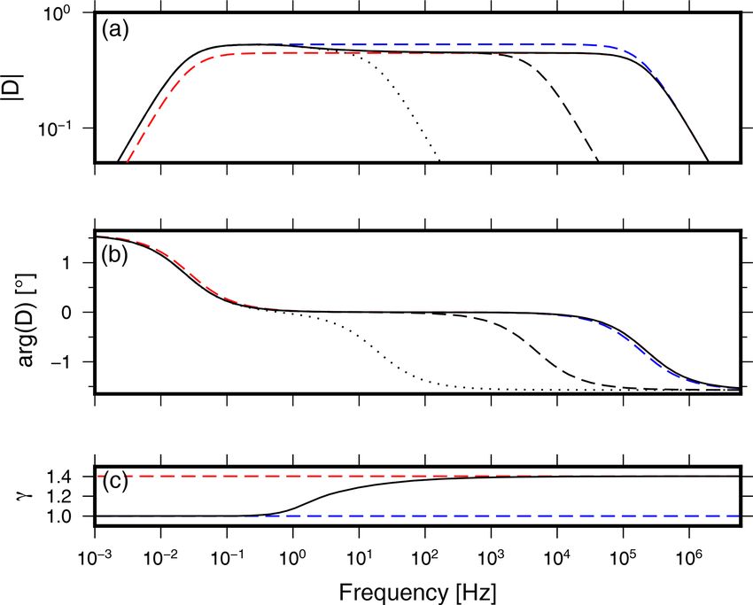
3306                                                                               O. F. C. den Ouden et al.: The INFRA-EAR

Figure 2. The KNMI mini-MB design with the DLVR sensor and the parameters as listed in Table 1 (a) and the electrical circuit of the
mini-MB (b). Panel (c) visualizes the DLVR sensor.

where η stands for the viscosity of air, which equals                 1. A broadband frequency response depends on a constant
18.27 µPa s at 18 ◦ C. Combining Eqs. (5) and (6) results in             pressure within the reference volume over the frequen-
the theoretical low-frequency cutoff:                                    cies of interest (i.e., τ1  τ2 ).

        Patm                                                          2. The pressure difference at the diaphragm is determined
fl ∼            .                                           (7)          by the relative acoustical resistances connected to the
       2π R2 V2
                                                                         sensor. The stability of the sensor response is assured by
Besides the high and low ends of the response, it is of in-              the capillary’s large resistance because of which R1
terest to determine the sensor response behavior within the              R2 .
passband (τ2−1 < ω < τ1−1 ).
                                                                      3. The sensor response depends on the ratio between the
                                                                       volumetric displacement of the diaphragm (Cd ) versus
D(iω) ∼ τ2−1 < ω < τ1−1                                                  the reference volume (C2 ). For the mini-MB, this term
                          1                                              can be neglected.
        =                                                   (8)
            1 + τ1 /τ2 + R1 /R2 + Cd /C2                               Figure 3 shows the theoretical sensor frequency response
                                                                    for amplitude (Fig. 3a) and phase (Fig. 3b) for isothermal
                | {z } | {z } | {z }
                    1     2         3
                                                                    (red) and adiabatic (blue) behavior. The transitional behav-
The three contributions in the denominator influence the            ior of the sensor response between isothermal and adiabatic
passband behavior of the sensor:                                    behavior will be discussed in the next section.

Atmos. Meas. Tech., 14, 3301–3317, 2021                                               https://doi.org/10.5194/amt-14-3301-2021
O. F. C. den Ouden et al.: The INFRA-EAR 3307
where
X = x (γadi − 1) − γadi , Y = y (γadi − 1) . (11)
x and y represent the real and imaginary components of a
complex-valued function Z δLt , which is dependent on the
geometrical shape of the enclosure and the thermal penetra-
tion depth. In between the adiabatic and isothermal limits,
the correction factor 3 describes the transition from an adia-
batic heat ratio (i.e., γ = 1.4) to an isothermal heat ratio, i.e.,
γ = 1. The transition frequency f defines the point where
the maximum correction of 3 occurs, i.e., for which δLt ≈ 1,
α
from which follows that f = πL 2.
In the case of the mini-MB, the fore and backing volume
have different shapes and sizes. The backing volume can be
described as a long cylinder, L2 , whereas the fore volume has
a rectangular shape, L1 . According to those geometries, the
Figure 3. The theoretical sensor frequency response function for transition frequency f of the fore and backing volume are 0.5
(a) amplitude and (b) phase in the case of isothermal and adia- and 2.2 Hz, respectively. Since f 1 ·τ1
1 and f 2 ·τ2
1 the
batic gas behavior in blue and red, respectively. The solid black line sensor response above τ1−1 is adiabatic, while the response
indicates the corrected sensor response by γ (c), as discussed in below τ2−1 is isothermal. Therefore, the thermal conduction
Sect. 3.1.3. The dotted and dashed lines indicate the high-frequency correction’s main effect is found to be in the passband region
shifting cutoff due to Rgore , as discussed in Sect. 3.1.4.
(Eq. 8).
The mini-MB has been designed to have a broadband re-
sponse; therefore, only the third term of the dominator is in-
3.1.3 Adiabatic–isothermal transition fluenced by the correction factor. The effect of thermal con-
duction to the response is due to ratio Cd , which means that
Due to the presence of heat conduction within the sensor, C2
air’s compressive behavior is neither isothermal nor adia- the correction factor is characterized by the geometric com-
batic. Instead, a transition from isothermal to adiabatic be- ponent of the backing volume:
havior is expected in the infrasonic frequency band (Richiar-
δt 2J1 (ζ )
done, 1993; Mentink and Evers, 2011). In the transition zone, Z = 1− , (12)
L ζ J0 (ζ )
the heat capacity ratio can be effectively described by
where Z indicates the characteristic correction √ assuming a
γ = 3γ , (9) long cylinder (Mentink and Evers, 2011). ζ = −2i δLt indi-
cates the ratio of L to δt , while J0 and J1 are the zeroth- and
where 3 indicates the correction factor to the heat capacity first-order Bessel functions of the first kind.
ratio γ . A difference in 3 will influence the capacitance val- The corrected theoretical sensor response is obtained by
ues of the fore and backing volumes (Eq. 3). C
substituting Cj = 3j . Figure 3c shows the value of γ in the
Whether a sound wave in an enclosure behaves isother- transaction zone between isothermal and adiabatic gas be-
mally or adiabatically depends on the size of the thermal pen- havior. The black line in Fig. 3a and b indicates the corrected
etration depth δt relative to characteristic length L of the en- theoretical sensor response.
closure. L is defined as the ratio between the enclosure’s vol- In the case of the mini-MB, the isothermal-to-adiabatic
ume and surface, i.e., L = VS . The thermal penetration depth transition results in an effect on the amplitude of 1|D| =
is specified as the gas layer thickness in which heat can dif- (γ − 1) Cd = 2.8 % and on the phase of less than a degree.
C2
fuse through q during the time of one wave period and is de-
Note that Cd
1 implies that the backing volume is rela-
rived as δt = 2α κ
ω , where α = ρcp indicates the thermal dif-
C2
tively large such that the change in gas behavior does not
fusivity, defined as the ratio of thermal conductivity (κ) and influence the sensitivity of the diaphragm.
heat capacity per unit volume (ρcp ). Adiabatic gas behavior
is obtained when δLt
1 and isothermal gas behavior when 3.1.4 Gore-Tex air vent
δt
L
1. The correction factor 3 is a function of δt /L and is
thus frequency dependent; it can be derived as As discussed in Sect. 3.1.2., the high- and low-frequency cut-
off are controlled by the resistivity of the inlet and backing
p π X volume, respectively. A Gore-Tex V9 sticker is added to the
|3| = X2 + Y 2 , arg(3) = + arctan , (10) opening of the casing’s pressure dome, which changes the
2 Y
https://doi.org/10.5194/amt-14-3301-2021 Atmos. Meas. Tech., 14, 3301–3317, 20213308 O. F. C. den Ouden et al.: The INFRA-EAR
resistivity of the inlets. The Gore-Tex V9 vent allows an air- of the measurement depends on the sensor’s internal error,
flow of 2×10⁻⁸ m3 s−1 m−2 . Poiseuille’s second law, Eq. (6), the self-noise. The self-noise corresponds to the diaphragm’s
shows the airflow resistivity caused by an open pipe and can deformation caused by the mass of the diaphragm plus the
be rewritten as electrical noise from the digitizer. As it is a digital sensor,
it is impossible to follow the conventional methods to deter-
1p
Rj = , (13) mine self-noise (Sleeman et al., 2006). Therefore the self-
qv noise is determined by opening both inlets to a closed pres-
sure chamber, ensuring no pressure difference between them.
where 1p indicates the pressure difference between both
The outcome stated that the self-noise falls within the sen-
sides of the pipe and qv the volumetric airflow.
sor’s maximum error band, ±0.7 Pa (DLVR, 2019). Since no
For the differential pressures that the mini-MB sensor is
backing volume is used, and the cavities at both sides of the
able to sense, ranging from 0.02 to 125 Pa, with a Gore-Tex
diaphragm are small, the relation Cd changes (Eq. 8). Due
air-vent area of 5 × 10⁻² m2 , the equivalent resistivity Rgore C2
ranges from 5 × 10⁵ to 3.125 × 10⁸ kg m−4 s−1 . Comparing to this, it is necessary to correct the sensor response for the
the resistivity of the air vent with the resistivity values of the adiabatic-to-isothermal transition. (Sect. 3.1.3).
capillary and the inlet of the sensor, Table 1 shows that the air The self-noise consistency is determined by calculating
vent will only influence the inlet’s resistivity. Assuming the the power spectral density (PSD) curves for each hour over
vent behaves linearly, the high-frequency cutoff of the sen- a test period of 24 h (Merchant and Hart, 2011). Figure 4a
sor decreases to a value of around 15 Hz. Figure 3 shows the shows in black the average 90th percentile confidence inter-
theoretical transfer function for the mini-MB with a Gore- val of the self-noise. Note that the instrumental self-noise ex-
Tex air vent attached to the inlet. The high-frequency cutoff ceeds the global low-noise model (Brown et al., 2014) at fre-
shifts between the dotted line and the dashed line due to vary- quencies above 0.4 Hz. Compared to high-fidelity equipment
ing values of Rgore . that typically falls entirely below the global low-noise mod-
els, such self-noise levels are relatively high, yet comparable
3.1.5 Experimental response to levels attained by similar sensor designs (Marcillo et al.,
2012). Furthermore, note that the self-noise follows the dy-
The theoretical sensor response describes the high- and low- namic range of a 12-bit ADC, as indicated by the gray dotted
frequency cutoff. Eq. (7) and the parameters listed in Table 1 line (Sleeman et al., 2006). The sensor has a maximum “no
show that the mini-MB has a theoretical low-frequency cut- missing code” of 12 bits, the effective number of bits (DLVR,
off of 0.042 Hz. A sudden over- or under-pressure (i.e., im- 2019).
pulse response) is applied to the sensor to determine the low-
frequency cutoff experimentally (Evers and Haak, 2000). 3.1.7 Sensor comparison
The impulse forces the diaphragm out of equilibrium. The
capillary and the size of the backing volume control the time A comparison between the mini-MB and a Hyperion IFS-
to return into equilibrium again. The time it takes for the di- 5111 sensor (Merchant, 2015) is made to assess the mini-MB
aphragm to reach equilibrium again corresponds to a char- performance relative to the reference Hyperion sensor. Both
acteristic relaxation time proportional to the low-frequency sensors have been placed inside a cabin next to the outside
cutoff. sensor test facility at the leading author’s institute. There is
The outcome of the experimental low-frequency cutoff a connection to the outside pressure field through air holes
was determined to be 0.044±0.0025 Hz. The theoretical low- in the wall of the cabin. The Hyperion sensor has been con-
frequency cutoff falls within the error margins of the exper- figured with a high-frequency shroud. Figure 4a and b show
imental cutoff frequency. The small difference between both the Probability Density Function (PDF) (Merchant and Hart,
is assumed to be due to experimental errors in timing the 2011) of the data recorded by the mini-MB and the Hyperion
relaxation time as well as small imperfections in the used sensor, respectively. Both sensors resolved the characteris-
capillary (Evers, 2008). It follows from Eq. (6) that the low- tic microbarom peak around 0.2 Hz (Christie and Campus,
frequency cutoff is inversely proportional to the radius to the 2010). The spectral peaks above 10 Hz correspond to reso-
fourth power. Hence, a 1 % deviation in the capillary radius nances that exist inside the measurement shelter.
will lead to a 4 % deviation in low-frequency cutoff. A direct comparison of the pressure recordings are shown
in Fig. 4c, d, and e. Figure 2c shows the absolute differ-
3.1.6 Sensor self-noise ence in amplitude over frequency, where panel d indicates
the phase difference between both sensors. Panel (e) shows
The resolution, the smallest change detectable by a sensor, the relative difference between the mini-MB and the Hyper-
depends on the sensor measurement range and the number of ion sensor. The sensors are in good agreement over the pass-
ADC bits. Having a linear response over a pressure range of band frequencies. A larger deviation is shown for the low-end
±125 Pa and a 14-bit built-in ADC results in a 0.02 Pa per (f < 0.07 Hz) and high-end frequencies(f > 8 Hz). At fre-
count resolution. Besides the ADC resolution, the accuracy quencies between 0.07 and 1 Hz, the pressure values are pos-
Atmos. Meas. Tech., 14, 3301–3317, 2021 https://doi.org/10.5194/amt-14-3301-2021O. F. C. den Ouden et al.: The INFRA-EAR 3309
Table 1. KNMI mini-MB components, parameter values, and standard conditions used in the computations.
KNMI mini-MB sensor specifications
Components Conditions
Inlet length l1 = 3 × 10⁻² m Ambient pressure Patm = 101 × 103 Pa
Inlet diameter a1 = 2 × 10⁻² m Isothermal gas constant γiso = 1
Capillary length l2 = 5 × 10⁻² m Adiabatic gas constant γadi = 1.403
Capillary diameter a2 = 1 × 10⁻⁴ m Thermal conductivity κ = 2.5 × 10⁻² W m−1 K−1
Diaphragm sensitivity Cd = 7.5 × 10⁻¹¹ m4 s2 kg−1 Heat capacity ρcp = 1.1 × 10³ J m−3 K−1
Parameters
Inlet resistance R1 = 8.7 × 10³ kg m−4 s−1 Fore volume V1 = 4.5 × 10⁻⁷ m 3
Capillary resistance R2 = 2.3 × 10¹⁰ kg m−4 s−1 Backing volume V2 = 16.5 × 10⁻⁶ m3
Size fore volume L1 = 2 × 10⁻⁴ m Size backing volume L2 = 4 × 10⁻⁴ m
Figure 4. PDFs of pressure spectra recorded with the mini-MB (a) and the Hyperion sensor (b) for a week of continuous recording in dB re
20−6 Pa2 Hz−1 . The dashed lines indicate the infrasonic high and low ambient noise levels (Brown et al., 2014). Panel (a) shows the PSD
of the 24 h self-noise recording of the mini-MB in black and the theoretical self-noise for a 12-, 13-, and 14-bit ADC as the gray dashed
lines. Panels (c) and (d) visualize the absolute difference T in amplitude and phase between the mini-MB and the Hyperion as a function
of frequency. Panel (e) displays the differences in sound pressure level measured by the mini-MB and the Hyperion sensor for the various
frequencies.
itively biased by 5 ± 1 dB, which equals a measurement error the relatively high noise level of the mini-MB. For the higher
by the KNMI mini-MB of ±0.005 Pa (Fig. 4e). Above 1 Hz, frequencies, the mini-MB PDF follows the 12-bit dynamic
the pressure values are biased by 10 ± 5 dB, which equals a range. Only in the case of significant events or loud ambi-
measurement error of ±0.02 Pa. ent noise, can the sensor sense pressure perturbations in the
The backing volume causes a deviation in the low- high-frequency range. Nonetheless, the mini-MB falls within
frequency spectrum. The high-frequency deviation is due to
https://doi.org/10.5194/amt-14-3301-2021 Atmos. Meas. Tech., 14, 3301–3317, 20213310 O. F. C. den Ouden et al.: The INFRA-EAR
a 30 dB error range over the entire frequency band compared WNRS filters cannot be attained. Not having a WNRS de-
to the Hyperion IFS-5111 sensor. creases the SNR; measuring wind with an anemometer will
give an insight into the wind conditions. Therefore, simulta-
3.2 Meteorological parameters neous measurement of wind and infrasound provides better
insight into the infrasonic SNR conditions.
The detectability of infrasound is directly linked to wind
noise conditions and the atmosphere’s stability in the infra- Sensor design
sound sensor’s surroundings since noise levels are increased
when turbulence levels are high. Therefore, it is beneficial to A 2D omnidirectional heat mass flow sensor has been de-
have simultaneous measurements of the basic meteorological signed to measure the wind conditions, which is a robust
parameters, i.e., pressure, wind, and temperature. The sub- and passive anemometer (Fig. 6a). The sensor is built with a
sections below describe the different meteorological mea- central heating element, which heats to approximately 80 ◦ C,
surements contained on the sensor platform. and is circularly surrounded by six TDK thermistors (TDK,
2018). Depending on the wind direction and speed, the tem-
3.2.1 Barometric pressure sensor perature field around the center element is modified. The
wind speed and direction can be estimated from the 2D tem-
The barometric pressure is sensed by the LPS33HW sensor
perature gradient, i.e., its absolute value and direction.
(STMicroelectronics, 2017), which is part of the pressure
dome. Similarly to the differential pressure sensor, piezo- Theoretical response
resistive crystals measure the barometric pressure.
Calibration tests are performed within a pressure cham- The six sensing elements are placed within a distance of 1 cm
ber in which a cycle of static pressures between 960 and from the heating element, while two thermistors and the heat-
1070 hPa can be produced. Besides the MEMS sensor, the ing element are at a spatial angle of 60◦ . The thermistors
chamber is equipped with a reference sensor. This procedure measure the temperature gradient caused by the wind flow
resulted in a calibration curve, which describes the pressure- since the resistance is strongly sensitive to temperature. The
dependent systematic bias. After correcting for the bias, the thermistors are made of semiconductor material and have
LPS sensor has an accuracy of ±0.1 hPa, i.e., the LPS sen- a negative temperature coefficient. The resistance decreases
sors measure values within ± 0.1 hPa of the value measured non-linearly with increasing temperature. The Steinhart–
by the KNMI reference sensor. Furthermore, the LPS sen- Hart equation approximately describes the temperature T as
sor has been field-tested (Fig. 5a), along with a Paroscien- a function of resistance value R (Steinhart and Hart, 1968):
tific Digiquartz 1015A barometer, which has an accuracy of
0.05 hPa. From the distribution of observations, it can be es- 1
timated that the LPS sensor has a precision of ±0.1 hPa for = C1 + C2 (ln(R )) + C3 ln(R )3 , (14)
T
93 % of the time (Fig. 5b). For the remainder, the maximum
deviation was ±0.15 hPa. where C1 , C2 , and C3 are the thermistor constants re-
ceived by the manufacturer (TDK, 2018). However, they can
3.2.2 Wind sensor as well be determined by taking three calibration measure-
ments, for which the temperature and resistance are known,
In addition to coherent acoustic signals, the pressure field and solving the three equations simultaneously. Figure 6b
at infrasonic frequencies consists to a large degree of pres- shows the sensitivity curve for the TDK thermistor. The ther-
sure perturbations due to wind and turbulence (Walker and mistor has a relative value of 1 at 25 ◦ C and a precision of
Hedlin, 2010). This turbulent energy is present over the com- ±4 % ◦ C−1 , which leads to a 0.05 ◦ C error. This error value
plete infrasonic frequency range with a typical noise ampli- is placed in context by modeling the expected temperate dif-
tude level decrease with increasing frequencies, following a ference under representative meteorological conditions in the
f −5/3 slope (Raspet et al., 2019). next section.
To reduce wind turbulence interference with the acoustic
perturbations, a wind-noise reduction system (WNRS) can Numerical sensor response
be put in place (Walker and Hedlin, 2010; Raspet et al.,
2019). Most WNRSs consist of a non-porous pipe rosette, The heating element needs to transfer a minimum tempera-
with low impedance inlets at each pipe’s end. All pipes are ture difference around the sensing elements (i.e., the sensing
connected to four main pipes, which connect to the micro- elements error). A numerical model has been built in ANSYS
barometer. By doing so, the atmosphere is sampled over a (ANSYS, 2018) to define the amount of temperature differ-
larger area and thus small incoherent pressure perturbations ence around the sensing elements under different meteoro-
(e.g., wind) are filtered out. logical circumstances. The model is a first approximation of
The sensor presented in this paper is designed for mobile the sensitivity and is based on homogeneous laminar airflow
sampling campaigns. In such cases, the application of similar passing by the sensor. Turbulent flow along the anemometer,
Atmos. Meas. Tech., 14, 3301–3317, 2021 https://doi.org/10.5194/amt-14-3301-2021O. F. C. den Ouden et al.: The INFRA-EAR 3311
Figure 5. A comparison between the barometric MEMS sensor (red) and a KNMI reference barometer (black). Panel (a) shows 5 d of
barometric pressure recordings using both sensors, while panel (b) displays the difference in measured barometric pressure by the MEMS
and the reference sensor.
Figure 6. Analyses of the anemometer. Panel (a) shows the top view of the sensor design, with the central heating element. Panel (b) indicates
the resistivity of the thermistors over temperature. The geometric sensitivity for the anemometer is shown in panel (c). The thermistors’
measured resistance for calibration setup 2 (90◦ ), for which the colors are in agreement with the sensor design (a), are shown in panel (d).
Panel (e) indicates the resolved wind direction and wind speed compared with the actual direction (dotted lines) and correct wind speed of
setups 1 (270◦ ), 2 (90◦ ), and 3 (60◦ ). The gray shaded area indicates the ±5◦ accuracy interval.
caused by the sensor design or casing, generates uncertain- Conversion of sensor output into atmospheric
ties within the measurements. parameters
This first approximation of sensitivity follows a numerical
forward modeling technique to approximate the heat probe’s
shape and intensity at a sensing element. The model was run To convert the measured resistivity into atmospheric param-
at stable meteorological parameters (i.e., 8 ◦ C air tempera- eters, a 2D planar temperature gradient has been estimated
ture, 50 % humidity, and 10 m s−1 wind speed). The outcome numerically from the discrete set of measurements. The mea-
shows that under those circumstances, the sensing element surement resistivities have been transformed into tempera-
experiences a temperature difference of around 4 ◦ C. To- ture measurements following Eq. (14). Based on those tem-
gether with the outcome of the thermistors’ sensitivity curve, peratures, a 2D numerical temperature gradient has been re-
it is concluded that the designed sensor can resolve this air- constructed. The problem is analogous to the estimation of
flow and is used to estimate wind speed and direction. the wavefront directivity from travel time differences (Szu-
berla and Olson, 2004).
In the present case, there are N = 6 discrete sample points,
each with an rj = (xj , yj ) coordinate and a temperature
value Tj . The total differential of the temperature describes
https://doi.org/10.5194/amt-14-3301-2021 Atmos. Meas. Tech., 14, 3301–3317, 20213312 O. F. C. den Ouden et al.: The INFRA-EAR
the variation of temperature T (x, y) as a function of x and y: that the mobile platform does not obstruct the laminar flow
in the tunnel.
∂T ∂T The calibration procedure consists of multiple indepen-
dT = dx + dy. (15)
∂x ∂y dent calibration tests that will be described next. First, the
sensor is placed inside the wind tunnel while there is no air-
From Eq.(15),
it follows that we can determine the 2D gradi-
∂T ∂T
flow. This way, the relative difference between the sensing
ent ∇T = ∂x , ∂y by setting up a system of N equations. elements is determined, the so-called zero measurement. The
In this case, the number of unknowns is two, and thus the sensor is corrected for the internal bias by correcting for the
gradient could be estimated by two measurements. However, relative difference, which varies around ±25 ohm. After cor-
in practice, errors are introduced due to measurement errors. recting the sensor bias, the sensor is placed within the hori-
Therefore the set of equations becomes inconsistent, which zontal plane (i.e., with a pitch angle of 0◦ ) at different angles
leads to nonsensical solutions. The unknown set of param- concerning the airflow. For every angle, the flow speed is var-
eters is solved by over-determining the system in a least- ied between 0 and 20 m s−1 .
squares sense to overcome this problem. Equation (15) can The calibration shows that the measured resistance of
be rewritten in terms of a matrix–vector system: the thermistors increases with increasing wind speeds. High
wind speeds increasingly cool down the thermistors, result-
y = Xp + , (16) ing in higher resistances. Figure 6d shows the six thermis-
tors’ measured resistance over the actual wind speed.
where y represents the temperature difference between two
The wind direction and the accuracy of the anemometers
measurement points, matrix X represents the M = N(N−1) 2 have been determined according to Eq. (17). Three differ-
pairwise separations, and p represents the temperature gra-
ent sensor setups show the accuracy and precision over in-
dient ∇T . It is assumed that the measurement errors can
creasing wind speeds as a function of directivity. The out-
be described by a normal distribution, i.e., a random vari-
come of calibration setups 1 (270◦ ), 2 (90◦ ), and 3 (60◦ ) are
able with mean E() = 0 and variance Var() = σ 2 . It can
shown, respectively, in Fig. 6e. The mean direction over all
be been shown that the least-squares estimate of p, here la-
wind speeds, for the three setups, is 89, 272, and 57◦ . The
beled p̂, can be obtained by solving the following equation:
standard deviation shows that the sensor’s accuracy is ±5◦ .
−1 Furthermore, it is shown that the precision of the wind di-
p̂ = X† X X† y (17) rection increases with increasing wind speeds. The resolved
p̂x p̂y wind speeds by the anemometer and the difference with the
px = , py = , (18) correct wind speed are shown in Fig. 6e. The colors indi-
p̂2x + pˆy 2 p̂2x + p̂2y
cate the difference between resolved wind speed and correct
where † represents the transpose operator. The solution sat- wind speed within the wind tunnel. The mean deviation be-
isfies Eq. (16) with the constraint that the sum of squared tween resolved and correct wind speed is ±2 m s−1 . Again,
errors is minimized. The matrix X and the error term deter- it is shown that the accuracy increases with increasing wind
mine the solution’s accuracy. If a Gaussian distribution can speeds.
represent the measurement errors, it can be shown that the
least-squares solution is unbiased. 3.3 Accelerometer
Based on the 2D reconstruction of the temperature gradi-
ent (Eq. 18), the wind direction and speed is resolved with an The sensing element of the infrasound sensor on this plat-
estimated accuracy. Furthermore, this method allows deter- form is a sensitive diaphragm. Strong accelerations of the
mining the uncertainty based on geometric sensor setup (Szu- platform will cause a deflection of the diaphragm and may
berla and Olson, 2004). Figure 6c shows the least-squares obscure infrasonic signal levels. In addition, such accelera-
error analyses of the sensor design (Fig. 6a). It stands out tions may be misinterpreted as infrasound if no independent
that the uncertainty increases when one element is positioned accelerometer information is available. To be able to separate
close to the wind flow (i.e., at 60◦ ). the mechanical response of the sensor from actual signals of
interest, the platform measures accelerations for which the
Reference calibration LSM303, a 6-axis inertial measurement unit (IMU), is de-
ployed (STMicroelectronics, 2018). The LSM303 consists of
Experimental calibration of the anemometer has been per- a 3-axis accelerometer and 3-axis magnetometer. The mea-
formed at the KNMI calibration lab. The calibration lab fea- surement range of the accelerometer varies between approx-
tures a wind tunnel, which generates a laminar airflow rang- imately 2–16 g. The magnetometer is out of the scope of this
ing between 0–20 m s−1 . Within the wind tunnel, two me- study and therefore neglected.
chanical anemometers are installed, which serve as reference Accelerometers measure differential movement between
sensors. With its MEMS anemometer, the mobile platform is the gravitational field vector and its reference frame. In the
installed right below one of the reference sensors to ensure absence of linear acceleration, the sensor measures the ro-
Atmos. Meas. Tech., 14, 3301–3317, 2021 https://doi.org/10.5194/amt-14-3301-2021O. F. C. den Ouden et al.: The INFRA-EAR 3313
tated gravitational field vector, which can be used to calibrate which makes it mobile and allows rapid deployments and
the sensor. A rotational movement of the sensor will result in measurements at remote places.
acceleration. The IMU is a digital sensor with a built-in 16- The INFRA-EAR is specifically designed to measure in-
bit ADC and has a resolution of 0.06 mg when choosing the frasound. The platform hosts the KNMI mini-MB, a novel
lowest measurement range. design with a pressure dome as inlet, the casing as backing
A comparison test has been carried out in the seismic volume with a PEEKsil capillary, and the DLVR-F50D as
pavilion of the author’s institute. Inside this pavilion, the the sensing element. The low-frequency cutoff of mini-MB
LSM is compared to a Streckeisen STS-2 seismometer con- depends on the size of the backing volume, and the capil-
nected to a Quanterra Q330 as a reference sensor (KNMI, lary characteristics. The high-frequency cutoff depends on
1993). Both sensors are installed on pillars to ensure a good the mini-MB inlet parameters, which is partly controlled by
coupling between the subsurface and the sensor. The com- a Gore-Tex air vent (Sect. 3.1.4). The infrasound logger has a
parison test, which is based on 24 h of recording, shows that low-frequency cutoff frequency of 0.044 ± 0.0025 Hz, while
the accuracy of the LSM303 3-axis accelerometer is ±1.5 mg the high-frequency cutoff varies between 15 and 90 Hz.
(1.5 cm s−2 ). Figure 7 shows the PDFs of the comparison test A comparison between the mini-MB and a Hyperion infra-
for the MEMS and STS-2 sensor. While the sensors are de- sound sensor (Merchant, 2015) has shown the differences in
ployed on the same seismic pillar and are thus subject to sim- amplitude and phase (Fig. 4). The mini-MB has an amplitude
ilar seismic noise conditions, the MEMS sensor could not difference of 30 dB for the passband frequencies band com-
measure ambient seismic noise (Peterson, 1993; McNamara pared to the Hyperion sensor. The sensors are in good agree-
and Buland, 2004) due to its high self-noise level. The LSM ment for the lower frequencies and both sensors resolved the
accelerometer exceeds both the U.S. Geological Survey New characteristic microbarom peak around 0.2 Hz (Christie and
High Noise Model (NHNM) (Peterson, 1993) and the STS-2 Campus, 2010). However, the higher frequencies show small
reference sensor by at least 35 dB. deviations, which is due to the relatively high noise band
It is therefore unlikely to use this IMU for monitoring pur- of the mini-MB. From 8 Hz onward, the mini-MB PDF fol-
poses of ambient seismic noise or teleseismic events. Pre- lows the 12-bit dynamic range of the ADC. Nonetheless, the
vious studies drew similar conclusions concerning the per- mini-MB can resolve the infrasonic ambient noise field up to
formance of MEMS accelerometers. Various calibration se- ±8 Hz. Only in the case of significant events or boisterous
tups are considered while comparing MEMS accelerometers conditions, can the sensor sense pressure perturbations in the
with conventional accelerometers of geophones (Hons et al., higher frequency range.
2008; Albarbar et al., 2009; Anthony et al., 2019), each con- When the wind-noise levels are high, infrasound signals
cluding that the accuracy of the MEMS is not sufficient for can be masked and remain undetected. Therefore, the sen-
recording ambient seismic noise. However, during strong lo- sor platform presents a passive anemometer to give insights
cal events or boisterous environments the MEMS sensor will into the wind conditions during infrasonic measurements.
resolve those seismic signals. The MEMS anemometer is built up as an omnidirectional
sensor. Numerical tests indicate that the temperature differ-
ence caused by a wind flow around the thermistors should be
significant to be sensed. For validation, the anemometer has
4 Discussion and conclusion been calibrated inside a wind tunnel. Figure 6 shows the out-
come of the calibration tests. Based on this outcome, one can
In this study, the constructional efforts and calibration pro- conclude that the anemometer can determine wind direction
tocols of the INFRA-EAR are presented. The INFRA-EAR and wind speed given that the sensor is calibrated. The sensor
is a low-cost mobile multidisciplinary sensor platform for measures a difference in resistance, which is converted into
the monitoring of geophysical quantities. It includes sensors a temperature measurement. The discreet temperature mea-
for the measurement of infrasound, acceleration, barometric surements are used to reconstruct a 2D planar temperature
pressure, and wind. gradient, which is used to determine the wind speed and di-
The platform uses the newest sensor technology, i.e., dig- rection. Based on the calibration tests within the wind tunnel,
ital MEMS, which have a built-in ADC. The MSP430 pro- it is shown that the anemometer has a directional accuracy of
grammable microcontroller unit controls the sampling of the ±5◦ and a wind speed accuracy of ±2 m s−1 . Nonetheless,
ADC and the storage of the data samples. A MEMS GPS is it is shown in Fig. 6c that the anemometer has geometrical
a unit to determine the positioning and to prevent clock drift. uncertainties due to it design. Future anemometers, 2D hot
Due to the small dimensions of MEMS and their low energy wire, should consider a minimum of eight thermistors to ex-
consumption, the “infrasound logger” is a pocket-size mea- clude geometric uncertainties (Szuberla and Olson, 2004).
surement platform, powered by an 1800 mAh lithium bat- Besides an anemometer and infrasound sensor, the plat-
tery. The platform does not require any infrastructure (e.g., form also hosts a barometric pressure sensor, an accelerome-
data connection, power supply, and specific mounting) as ter, and GPS. Each sensor has been calibrated and compared
commonly used for the deployment of high-fidelity systems, with a reference sensor. It was shown that the accelerome-
https://doi.org/10.5194/amt-14-3301-2021 Atmos. Meas. Tech., 14, 3301–3317, 2021You can also read