The Met Office Unified Model Global Atmosphere 7.0/7.1 and JULES Global Land 7.0 configurations - GMD
←
→
Page content transcription
If your browser does not render page correctly, please read the page content below
Geosci. Model Dev., 12, 1909–1963, 2019
https://doi.org/10.5194/gmd-12-1909-2019
© Author(s) 2019. This work is distributed under
the Creative Commons Attribution 4.0 License.

The Met Office Unified Model Global Atmosphere 7.0/7.1 and
JULES Global Land 7.0 configurations
David Walters1 , Anthony J. Baran1,2 , Ian Boutle1 , Malcolm Brooks1 , Paul Earnshaw1 , John Edwards1 ,
Kalli Furtado1 , Peter Hill3 , Adrian Lock1 , James Manners1 , Cyril Morcrette1 , Jane Mulcahy1 , Claudio Sanchez1 ,
Chris Smith1 , Rachel Stratton1 , Warren Tennant1 , Lorenzo Tomassini1 , Kwinten Van Weverberg1 , Simon Vosper1 ,
Martin Willett1 , Jo Browse4 , Andrew Bushell1 , Kenneth Carslaw7 , Mohit Dalvi1 , Richard Essery5 , Nicola Gedney6 ,
Steven Hardiman1 , Ben Johnson1 , Colin Johnson1 , Andy Jones1 , Colin Jones8 , Graham Mann7,8 , Sean Milton1 ,
Heather Rumbold1 , Alistair Sellar1 , Masashi Ujiie9 , Michael Whitall1 , Keith Williams1 , and Mohamed Zerroukat1
1 Met Office, FitzRoy Road, Exeter, EX1 3PB, UK
2 School of Physics, Astronomy and Mathematics, University of Hertfordshire, Hatfield, AL10 9AB, UK
3 Department of Meteorology, University of Reading, Reading, RG6 6BB, UK
4 Centre for Geography, Society and the Environment, University of Exeter – Penryn Campus, Cornwall, TR10 9EZ, UK
5 School of Geosciences, University of Edinburgh, Edinburgh, EH8 9XP, UK
6 Met Office, Joint Centre for Hydrometeorological Research, Maclean Building, Wallingford, OX10 8BB, UK
7 School of Earth and Environment, University of Leeds, Leeds, LS2 9JT, UK
8 National Centre for Atmospheric Science, University of Leeds, Leeds, LS2 9JT, UK
9 Numerical Prediction Division, Japan Meteorological Agency, 1-3-4 Otemachi, Chiyoda-ku, Tokyo 100-8122, Japan

Correspondence: David Walters (david.walters@metoffice.gov.uk)

Received: 15 November 2017 – Discussion started: 28 November 2017
Revised: 15 February 2018 – Accepted: 20 March 2018 – Published: 14 May 2019

Abstract. We describe Global Atmosphere 7.0 and Global               In addition, we describe the GA7.1 branch configura-
Land 7.0 (GA7.0/GL7.0), the latest science configurations of      tion, which reduces an overly negative anthropogenic aerosol
the Met Office Unified Model (UM) and the Joint UK Land           effective radiative forcing (ERF) in GA7.0 whilst main-
Environment Simulator (JULES) land surface model devel-           taining the quality of simulations of the present-day cli-
oped for use across weather and climate timescales. GA7.0         mate. GA7.1/GL7.0 will form the physical atmosphere/land
and GL7.0 include incremental developments and targeted           component in the HadGEM3–GC3.1 and UKESM1 climate
improvements that, between them, address four critical er-        model submissions to the CMIP6.
rors identified in previous configurations: excessive precipi-
tation biases over India, warm and moist biases in the tropical
tropopause layer (TTL), a source of energy non-conservation
in the advection scheme and excessive surface radiation bi-       1   Introduction
ases over the Southern Ocean. They also include two new
parametrisations, namely the UK Chemistry and Aerosol             In this paper, we document the Global Atmosphere 7.0 con-
(UKCA) GLOMAP-mode (Global Model of Aerosol Pro-                  figuration (GA7.0) of the Met Office Unified Model (UM;
cesses) aerosol scheme and the JULES multi-layer snow             Brown et al., 2012) and the Global Land 7.0 configura-
scheme, which improve the fidelity of the simulation and          tion (GL7.0) of the Joint UK Land Environment Simulator
were required for inclusion in the Global Atmosphere/Global       (JULES) land surface model (Best et al., 2011; Clark et al.,
Land configurations ahead of the 6th Coupled Model Inter-         2011). These are the latest iterations in the line of GA/GL
comparison Project (CMIP6).                                       configurations developed for use in global atmosphere/land
                                                                  and coupled modelling systems across weather and climate

Published by Copernicus Publications on behalf of the European Geosciences Union.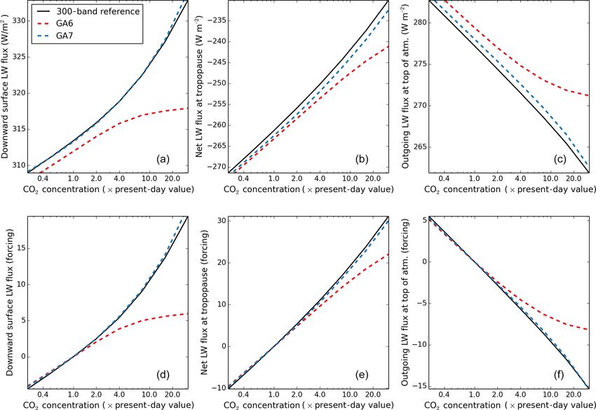
1910                                                      D. Walters et al.: UM GA7.0/GA7.1 and JULES GL7.0 configurations

timescales. This development is a continual process made               so for consistency with that documentation, we list the trac
up of small incremental changes to parameters and options              ticket numbers (denoted by trac’s # character) along with
within existing parametrisation schemes, the implementation            these descriptions. Section 4 includes an assessment of the
of new schemes and options, and less frequent major changes            configuration’s performance in global weather prediction and
to the structure of the model and the framework on which it            atmosphere/land-only climate simulations. This illustrates
is built. The Global Atmosphere 6.0 configuration (GA6.0;              the reduction of the critical model errors noted above, and
Walters et al., 2017) fell into the latter category, as it included    highlights some improvements in simple weather prediction
a once-in-a-decade replacement of the model’s dynamical                tests, but suggests that improvements are needed in the inter-
core. To allow the configuration developers to concentrate             action between the model and its data assimilation before im-
on that change, the inclusion of other changes was limited             plementation for operational forecasting. In Sect. 5 we briefly
to those that were known to be necessary alongside the dy-             describe GA7.1, which is based on the GA7.0 “trunk” config-
namical core, or to significantly improve system performance           uration but includes a minimal set of changes for addressing
measures, so as to make the dynamical core implementation              the excessive aerosol forcing discussed in Sect. 4.5. As a re-
easier. For this reason, GA7 sees the inclusion of a number            sult of this work, GA7.1 and GL7.0 are suitable for use as the
of bottom-up developments to the atmospheric parametrisa-              physical atmosphere and land components in the HadGEM3–
tion schemes developed over several years that improve the             GC3.1 and UKESM1 climate models that will be submitted
fidelity and internal consistency of the model. These include          to the CMIP6.
an improved treatment of gaseous absorption in the radiation
scheme, improvements to the treatment of warm rain and ice
cloud, and an improvement to the numerics in the model’s               2     Global Atmosphere 7.0 and Global Land 7.0
convection scheme. It also includes a number of top-down
developments motivated by the findings of process evalu-               2.1    Dynamical formulation and discretisation
ation groups (PEGs), which are tasked with understanding
                                                                       The UM’s ENDGame dynamical core uses a semi-implicit
the root causes of model error. These changes include fur-
                                                                       semi-Lagrangian formulation to solve the non-hydrostatic,
ther developments in the model’s microphysics and incre-
                                                                       fully compressible deep-atmosphere equations of mo-
mental improvements to our implementation of the dynami-
                                                                       tion (Wood et al., 2014). The primary atmospheric prog-
cal core. In combination with the bottom-up developments
                                                                       nostics are the three-dimensional wind components, virtual
discussed previously, these lead to large reductions in our
                                                                       dry potential temperature, Exner pressure and dry density,
four critical model errors, namely rainfall deficits over India
                                                                       whilst moist prognostics such as the mass mixing ratio of
during the South Asian monsoon, temperature and humid-
                                                                       water vapour and prognostic cloud fields as well as other
ity biases in the tropical tropopause layer (TTL), deficiencies
                                                                       atmospheric loadings are advected as free tracers. These
in the model’s numerical conservation and surface flux bi-
                                                                       prognostic fields are discretised horizontally onto a regu-
ases over the Southern Ocean. Finally, GA7 and GL7 include
                                                                       lar longitude–latitude grid with Arakawa C-grid stagger-
new parametrisation schemes, which increase the complex-
                                                                       ing (Arakawa and Lamb, 1977), whilst the vertical discreti-
ity and fidelity of the model and introduce new functionality
                                                                       sation utilises a Charney–Phillips staggering (Charney and
that was deemed necessary for the next generation climate
                                                                       Phillips, 1953) using terrain-following hybrid height coor-
modelling systems in which they will be used and which will
                                                                       dinates. The discretised equations are solved using a nested
form the UK’s contribution to the 6th Coupled Model Inter-
                                                                       iterative approach centred about solving a linear Helmholtz
comparison Project (CMIP6; Eyring et al., 2015). These new
                                                                       equation. By convention, global configurations are defined
capabilities include a multi-moment modal representation of
                                                                       on 2× N longitudinal columns and 1.5× N latitudinal rows
prognostic tropospheric aerosols, a multi-layer snow scheme
                                                                       of grid points for scalar variables, with the meridional wind
and a seamless stochastic physics package, which will over-
                                                                       variable held at the north and south poles and scalar and
see the inclusion of stochastic physics terms in production
                                                                       zonal wind variables first stored half a grid length away from
UM climate simulations for the first time.
                                                                       the poles. This choice makes the grid-spacing approximately
   In Sect. 2 we describe GA7.0 and GL7.0, whilst in Sect. 3
                                                                       isotropic in the mid-latitudes and means that the integer N ,
we document how these differ from the last documented con-
                                                                       which represents the maximum number of zonal 2 grid-point
figurations: GA6.0 and GL6.01 . The development of these
                                                                       waves that can be represented by the model, uniquely de-
changes is documented using “trac” issue tracking software,
                                                                       fines its horizontal resolution; a model with N = 96 is said
                                                                       to have N96 resolution. Limited-area configurations use a
    1 Where     the configurations remain unchanged from               rotated longitude–latitude grid with the pole rotated so that
GA6.0/GL6.0 and their predecessors, Sect. 2 contains mate-             the grid’s equator runs through the centre of the model do-
rial which is unaltered from the documentation papers for those        main. In the vertical, the majority of climate configurations
releases (i.e. Walters et al., 2011; Walters et al., 2014; Walters
et al., 2017). In addition to the material herein, the Supplement to   definition that are dependent on either model resolution or system
this paper includes a short list of model settings outside the GA/GL   application.

Geosci. Model Dev., 12, 1909–1963, 2019                                                  www.geosci-model-dev.net/12/1909/2019/
D. Walters et al.: UM GA7.0/GA7.1 and JULES GL7.0 configurations                                                             1911

Table 1. Typical time step for a range of horizontal resolutions.   rithm 1. In practice two iterations are used for each of the
                                                                    outer and inner loops so that the Helmholtz problem is solved
                             Nominal       Typical                  4 times per time step. The prognostic aerosol scheme is in-
                            horizontal       time                   cluded via a call to the UK Chemistry and Aerosol (UKCA)
                 Grid       resolution        step                  code after the main atmospheric time step; this call is cur-
                 N96           135 km     20.0 min                  rently performed once per hour. Finally, Table 1 contains the
                 N216           60 km     15.0 min                  typical length of time step used for a range of horizontal res-
                 N320           40 km     12.0 min                  olutions.
                 N512           25 km     10.0 min
                 N640           20 km      7.5 min
                 N768           17 km      7.5 min
                 N1280          10 km      4.0 min

use an 85-level set labelled L85(50t , 35s )85 , which has 50
levels below 18 km (and hence at least sometimes in the
troposphere), 35 levels above this (and hence solely in or
above the stratosphere) and a fixed model lid 85 km above
sea level. Limited-area climate simulations use a reduced
63-level set, L63(50t , 13s )40 , which has the same 50 levels
below 18 km, with only 13 above and a lower model top
at 40 km. Finally, numerical weather prediction (NWP) con-
figurations use a 70-level set, L70(50t , 20s )80 which has an
almost identical 50 levels below 18 km and a model lid at
80 km but has a reduced stratospheric resolution compared
to L85(50t , 35s )85 . Although we use a range of vertical reso-
lutions in the stratosphere, a consistent tropospheric vertical
resolution is currently used for a given GA configuration. A
more detailed description of these level sets is included in the
Supplement to this paper.

2.2   Structure of the atmospheric model time step

With ENDGame, the UM uses a nested iterative structure for
each atmospheric time step within which processes are split
into an outer loop and an inner loop. The semi-Lagrangian           2.3   Solar and terrestrial radiation
departure point equations are solved within the outer loop
using the latest estimates for the wind variables. Appropriate      Shortwave (SW) radiation from the Sun is absorbed and re-
fields are then interpolated to the updated departure points.       flected in the atmosphere and at the Earth’s surface and pro-
Within the inner loop, the Coriolis, orographic and non-linear      vides energy to drive the atmospheric circulation. Longwave
terms are solved along with a linear Helmholtz problem to           (LW) radiation is emitted from the planet and interacts with
obtain the pressure increment. Latest estimates for all vari-       the atmosphere, redistributing heat, before being emitted into
ables are then obtained from the pressure increment via a           space. These processes are parametrised via the radiation
back-substitution process; see Wood et al. (2014) for details.      scheme, which provides prognostic atmospheric temperature
The physical parametrisations are split into slow processes         increments, prognostic surface fluxes and additional diag-
(radiation, large-scale precipitation and gravity-wave drag –       nostic fluxes. The SOCRATES (https://code.metoffice.gov.
GWD) and fast processes (atmospheric boundary-layer tur-            uk/trac/socrates, last access: 4 April 2019) radiative transfer
bulence, convection and land surface coupling). The slow            scheme (Edwards and Slingo, 1996; Manners et al., 2015)
processes are treated in parallel and are computed once per         is used with a new configuration for GA7. Solar radiation
time step before the outer loop. The source terms from the          is treated in six SW bands and thermal radiation in nine
slow processes are then added on to the appropriate fields be-      LW bands, as outlined in Table 2. Gaseous absorption uses
fore interpolation. The fast processes are treated sequentially     the correlated-k method with newly derived coefficients for
and are computed in the outer loop using the latest predicted       all gases (except where indicated below) based on the HI-
estimate for the required variables at the next, n+1 time step.     TRAN 2012 spectroscopic database (Rothman et al., 2013).
A summary of the atmospheric time step is given in Algo-            Scaling of absorption coefficients uses a lookup table of 59

www.geosci-model-dev.net/12/1909/2019/                                                Geosci. Model Dev., 12, 1909–1963, 2019
1912                                                 D. Walters et al.: UM GA7.0/GA7.1 and JULES GL7.0 configurations

pressures with five temperatures per pressure level based         wide range of plausible Mie parameters and stored in lookup
around a mid-latitude summer profile. The method of equiv-        tables for use during run time when the atmospheric chem-
alent extinction (Edwards, 1996; Amundsen et al., 2017)           ical composition, including the mean aerosol particle radius
is used for minor gases in each band. The water vapour            and water content, are known. As the aerosol species are in-
continuum is represented using laboratory results from the        ternally mixed within the modal aerosol scheme (see Table 4)
CAVIAR project (Continuum Absorption at Visible and In-           the refractive indices of each mode are calculated online as a
frared wavelengths and its Atmospheric Relevance) between         volume-weighted mean of the component species contribut-
1 and 5 µm (Ptashnik et al., 2011, 2012) and version 2.5          ing to that mode. The component refractive indices are doc-
of the Mlawer–Tobin–Clough–Kneizys–Davies (MT_CKD-                umented in the Appendix of Bellouin et al. (2013). Nucle-
2.5) model (Mlawer et al., 2012) at other wavelengths.            ation mode particles are neglected, as they are not expected
   Forty-one (41) k terms are used for the major gases in the     to contribute significantly to the atmospheric optical prop-
SW bands. Absorption by water vapour (H2 O), carbon diox-         erties. The parametrisation of cloud droplets is described in
ide (CO2 ), ozone (O3 ), oxygen (O2 ), nitrous oxide (N2 O) and   Edwards and Slingo (1996) using the method of “thick aver-
methane (CH4 ) is included. Ozone cross sections for the ul-      aging”. Padé fits are used for the variation with effective ra-
traviolet (UV) and visible bands come from Serdyuchenko           dius, which is computed from the number of cloud droplets.
et al. (2014) and Gorshelev et al. (2014), along with Brion–      In configurations using prognostic aerosol, cloud droplet
Daumont–Malicet (Daumont et al., 1992; Malicet et al.,            number concentrations are not calculated within the radia-
1995) for the far UV. In the first SW band, a single k term is    tion scheme itself but are calculated by the UKCA-Activate
calculated for each 20 nm sub-interval from 200 to 320 nm,        scheme (West et al., 2014), which is based on the activation
and in band 2, a single k term is calculated for each of the      scheme of Abdul-Razzak and Ghan (2000). Note that in sim-
sub-intervals, 320–400 and 400–505 nm. This allows the in-        ulations using climatological rather than prognostic aerosol,
coming solar flux to be supplied on these finer wavelength        the approach described here is not yet available, and instead
bands for experiments concerning solar spectral variability.      we use CLASSIC (Coupled Large-scale Aerosol Simulator
The solar spectrum uses data from the Naval Research Labo-        for Studies in Climate; Bellouin et al., 2011) aerosol clima-
ratory Solar Spectral Irradiance model (NRLSSI; Lean et al.,      tologies and the calculation of optical properties and cloud
2005) as recommended by the SPARC/SOLARIS (Solar In-              droplet concentrations described in Sect. 2.3 of Walters et al.
fluences for SPARC: Stratospheric Processes and their Role        (2017). Both prognostic and climatological simulations of
in Climate; http://solarisheppa.geomar.de/ccmi, last access:      mineral dust also use the CLASSIC scheme. This is dis-
4 April 2019) group. A mean solar spectrum for the period         cussed in more detail in Sect. 3.8. The parametrisation of ice
2000–2011 is used when a varying spectrum is not invoked.         crystals is described in Baran et al. (2016). Full treatment of
   Eighty-one (81) k terms are used for the major gases in the    scattering is used in both the SW and LW. The sub-grid cloud
LW bands. Absorption by H2 O, O3 , CO2 , CH4 , N2 O, CFC-         structure is represented using the Monte Carlo independent
11 (CCl3 F), CFC-12 (CCl2 F2 ) and HFC134a (CH2 FCF3 ) is         column approximation (McICA) as described in Hill et al.
included. For climate simulations, the atmospheric concen-        (2011), with the parametrisation of sub-grid-scale water con-
trations of CFC-12 and HFC134a are adjusted to represent          tent variability described in P. G. Hill et al. (2015).
absorption by all the remaining trace halocarbons. The treat-        Full radiation calculations are made every hour using the
ment of CO2 absorption for the peak of the 15 µm band (LW         instantaneous cloud fields and a mean solar zenith angle for
band 4) is as described in Zhong and Haigh (2000). An im-         the following 1 h period. Corrections are made for the change
proved representation of CO2 absorption in the “window”           in solar zenith angle on every model time step as described
region (8–13 µm) provides a better forcing response to in-        in Manners et al. (2009). The emissivity and the albedo of
creases in CO2 (Pincus et al., 2015). The method of “hybrid”      the surface are set by the land surface model. The direct SW
scattering is used in the LW, which runs full scattering calcu-   flux at the surface is corrected for the angle and aspect of the
lations for 27 of the major gas k terms (where their nominal      topographic slope as described in Manners et al. (2012).
optical depth is less than 10 in a mid-latitude summer atmo-
sphere). For the remaining 54 k terms (optical depth > 10)        2.4   Large-scale precipitation
much cheaper non-scattering calculations are run.
   Of the major gases considered, only H2 O is prognostic;        The formation and evolution of precipitation due to grid scale
O3 uses a zonally symmetric climatology, whilst other gases       processes is the responsibility of the large-scale precipitation
are prescribed using either fixed or time-varying mass mixing     – or microphysics – scheme, whilst small-scale precipitat-
ratios and are assumed to be well mixed.                          ing events are handled by the convection scheme. The micro-
   Absorption and scattering by the following prognostic          physics scheme has prognostic input fields of temperature,
aerosol species are included in both the SW and LW using the      moisture, cloud and precipitation from the end of the previ-
UKCA-Radaer scheme: sulfate, black carbon, organic car-           ous time step, which it modifies in turn. The microphysics
bon and sea salt. The aerosol scattering and absorption co-       used is a single-moment scheme based on Wilson and Bal-
efficients and asymmetry parameters are pre-computed for a        lard (1999), with extensive modifications. The warm rain

Geosci. Model Dev., 12, 1909–1963, 2019                                             www.geosci-model-dev.net/12/1909/2019/
D. Walters et al.: UM GA7.0/GA7.1 and JULES GL7.0 configurations                                                                1913

Table 2. Spectral bands for the treatment of incoming solar (SW) radiation (left) and thermal (LW) radiation (right).

                    SW
                    Band     Wavelength (nm)      LW Band         Wave number (cm−1 )                  Wavelength (µm)
                    1               200–320               1                    1–400                        25–10 000
                    2               320–505               2                  400–550                         18.18–25
                    3               505–690               3      550–590 and 750–800       12.5–13.33 and 16.95–18.18
                    4              690–1190               4                  590–750                      13.33–16.95
                    5             1190–2380               5    800–990 and 1120–1200         8.33–8.93 and 10.10–12.5
                    6            2380–10 000              6                 990–1120                       8.93–10.10
                    –                      –              7                1200–1330                        7.52–8.33
                    –                      –              8                1330–1500                        6.67–7.52
                    –                      –              9                1500–2995                        3.34–6.67

scheme is based on Boutle et al. (2014b) and includes a prog-            parametrisation described in Van Weverberg et al. (2016).
nostic rain formulation, which allows three-dimensional ad-              PC2 uses three prognostic variables for the water mixing
vection of the precipitation mass mixing ratio and an ex-                ratio – vapour, liquid and ice – and a further three prog-
plicit representation of the effect of sub-grid variability on           nostic variables for the cloud fraction – liquid, ice and
autoconversion and accretion rates (Boutle et al., 2014a).               mixed phase. The following atmospheric processes can mod-
We use the rain-rate-dependent particle size distribution of             ify the cloud fields: SW radiation, LW radiation, boundary-
Abel and Boutle (2012) and fall velocities of Abel and Ship-             layer processes, convection, precipitation, small-scale mix-
way (2007), which combine to allow a better representation               ing (cloud erosion), advection and changes in atmospheric
of the sedimentation and evaporation of small droplets. We               pressure. The convection scheme calculates increments to the
also make use of multiple sub-time steps of the precipita-               prognostic liquid and ice water contents by detraining con-
tion scheme, with one call to the scheme for every 2 minutes             densate from the convective plume, whilst the cloud fractions
of the model time step. This is required to achieve a realistic          are updated using the non-uniform forcing method of Bushell
treatment of in-column evaporation. With prognostic aerosol,             et al. (2003). One advantage of the prognostic approach is
we use the UKCA-Activate aerosol activation scheme (West                 that cloud can be transported away from where it was cre-
et al., 2014) to provide the cloud droplet number for auto-              ated. For example, anvils detrained from convection can per-
conversion, where only soluble aerosol species (which can                sist and be advected downstream long after the convection
be composed of sulfate, sea salt, black carbon and organic               itself has ceased. The radiative impact of convective cores,
carbon) contribute to the droplet number. When using clima-              which hold condensate not detrained into the environment, is
tological aerosol, the cloud droplet number is the same as               represented by diagnosing a convective cloud amount (CCA)
that used in the radiation scheme. Ice cloud parametrisations            and convective cloud water (CCW) where the convection is
use the generic size distribution of Field et al. (2007) and             active on a particular time step. The CCA and CCW then
mass–diameter relations of Cotton et al. (2013).                         get combined with the PC2 cloud fraction and condensate
                                                                         variables before these get passed to McICA to calculate the
2.5   Large-scale cloud                                                  radiative impact of the combined cloud fields. Finally, the
                                                                         production of supercooled liquid water in a turbulent envi-
Cloud appears on sub-grid scales well before the humidity                ronment is parametrised following Furtado et al. (2016).
averaged over the size of a model grid box reaches saturation.
A cloud parametrisation scheme is therefore required to de-              2.6   Sub-grid orographic drag
termine the fraction of the grid box which is covered by cloud
and the amount and phase of condensed water contained in                 The effect of local and mesoscale orographic features not
this cloud. The formation of cloud will convert water vapour             resolved by the mean orography, from individual hills to
into liquid or ice and release latent heat. The cloud cover and          small mountain ranges, must be parametrised. The smallest
liquid and ice water contents are then used by the radiation             scales, where buoyancy effects are not important, are repre-
scheme to calculate the radiative impact of the cloud and by             sented by an effective roughness parametrisation in which
the large-scale precipitation scheme to calculate whether any            the roughness length for momentum is increased above the
precipitation has formed.                                                surface roughness to account for the additional stress due to
   The parametrisation used is the prognostic cloud frac-                the sub-grid orography (Wood and Mason, 1993). The effects
tion and prognostic condensate (PC2) scheme (Wilson et al.,              of the remainder of the sub-grid orography (on scales where
2008a, b) along with the cloud erosion parametrisation de-               buoyancy effects are important) are parametrised by a drag
scribed by Morcrette (2012) and critical relative humidity               scheme which represents the effects of low-level-flow block-

www.geosci-model-dev.net/12/1909/2019/                                                       Geosci. Model Dev., 12, 1909–1963, 2019
1914                                                  D. Walters et al.: UM GA7.0/GA7.1 and JULES GL7.0 configurations

ing and the drag associated with stationary gravity waves          propagation, to match the locally evaluated saturation spec-
(mountain waves). This is based on the scheme described by         trum.
Lott and Miller (1997) but with some important differences,
described in more detail in Vosper (2015).                         2.8   Atmospheric boundary layer
   The sub-grid orography is assumed to consist of uni-
formly distributed elliptical mountains within the grid box,       Turbulent motions in the atmosphere are not resolved by
described in terms of a height amplitude, which is propor-         global atmospheric models but are important to parametrise
tional to the grid-box standard deviation of the source orog-      in order to give realistic vertical structure in the thermo-
raphy data, anisotropy (the extent to which the sub-grid orog-     dynamic and wind profiles. Although referred to as the
raphy is ridge like, as opposed to circular), the alignment of     “boundary-layer” scheme, this parametrisation represents
the major axis and the mean slope along the major axis. The        mixing over the full depth of the troposphere. The scheme is
scheme is based on two different frameworks for the drag           that of Lock et al. (2000) with the modifications described in
mechanisms: bluff body dynamics for the flow-blocking and          Lock (2001) and Brown et al. (2008). It is a first-order turbu-
linear gravity waves for the mountain-wave drag component.         lence closure mixing adiabatically conserved heat and mois-
   The degree to which the flow is blocked and so passes           ture variables, momentum and tracers. For unstable bound-
around, rather than over the mountains is determined by the        ary layers, diffusion coefficients (K profiles) are specified
Froude number, F = U/(N H ) where H is the assumed sub-            functions of height within the boundary layer, related to the
grid mountain height (proportional to the sub-grid standard        strength of the turbulence forcing. Two separate K profiles
deviation of the source orography data) and N and U are            are used, one for surface sources of turbulence (surface heat-
respectively measures of the buoyancy frequency and wind           ing and wind shear) and one for cloud-top sources (radia-
speed of the low-level flow. When F is less than the crit-         tive and evaporative cooling). The existence and depth of
ical value, Fc , a fraction of the flow is assumed to pass         unstable layers is diagnosed initially by two moist adiabatic
around the sides of the orography, and a drag is applied to        parcels, one released from the surface, the other from cloud-
the flow within this blocked layer. Mountain waves are gen-        top. The top of the K profile for surface sources and the
erated by the remaining proportion of the layer which the          base of that for cloud-top sources are then adjusted to en-
orography pierces through. The acceleration of the flow due        sure that, from the resultant buoyancy flux, the magnitude
to wave stress divergence is exerted at levels where wave          of the buoyancy consumption of turbulence kinetic energy
breaking is diagnosed. The kinetic energy dissipated through       is limited to a specified fraction of buoyancy production,
the flow-blocking drag, the mountain-wave drag and the non-        integrated across the boundary layer. This can permit the
orographic gravity-wave drag (see Sect. 2.7 below) is re-          cloud layer to decouple from the surface (Nicholls, 1984).
turned to the atmosphere as a local heating term.                  This same energetic diagnosis is used to limit the vertical
                                                                   extent of the surface-driven K profile when cumulus con-
2.7    Non-orographic gravity-wave drag                            vection is diagnosed (through comparison of cloud and sub-
                                                                   cloud layer moisture gradients), except that in this case no
Non-orographic sources – such as convection, fronts and jets       condensation is included in the diagnosed buoyancy flux be-
– can force gravity waves with non-zero phase speed. These         cause that part of the distribution is handled by the convec-
waves break in the upper stratosphere and mesosphere, de-          tion scheme (which is triggered at the cloud base). Mixing
positing momentum, which contributes to driving the zonal          across the top of the boundary layer is through an explicit en-
mean wind and temperature structures away from radia-              trainment parametrisation that can either be resolved across
tive equilibrium. Waves on scales too small for the model          a diagnosed inversion thickness or, if too thin, is coupled to
to sustain explicitly are represented by a spectral sub-grid       the radiative fluxes and the dynamics through a sub-grid in-
parametrisation scheme (Scaife et al., 2002), which by con-        version diagnosis. If the thermodynamic conditions are right,
tributing to the deposited momentum leads to a more realistic      cumulus penetration into a stratocumulus layer can generate
tropical quasi-biennial oscillation (QBO). The scheme, de-         additional turbulence and cloud-top entrainment in the stra-
scribed in more detail in Walters et al. (2011), represents pro-   tocumulus by enhancing evaporative cooling at the cloud top.
cesses of wave generation, conservative propagation and dis-       There are additional non-local fluxes of heat and momentum
sipation by critical-level filtering and wave saturation acting    in order to generate more vertically uniform potential tem-
on a vertical wave number spectrum of gravity-wave fluxes          perature and wind profiles in convective boundary layers.
following Warner and McIntyre (2001). Momentum conser-             Primarily for stable boundary layers and in the free tropo-
vation is enforced at launch in the lower troposphere, where       sphere, diffusion coefficients are also calculated using a lo-
isotropic fluxes guarantee zero net momentum, and by im-           cal Richardson number scheme based on Smith (1990), with
posing a condition of zero vertical wave flux at the model’s       the final coefficients being the maximum of this and the non-
upper boundary. In between, momentum deposition occurs in          local ones described above. The stability dependence in un-
each layer where reduced integrated flux results from erosion      stable boundary layers uses the “conventional function” of
of the launch spectrum, after transformation by conservative       Brown (1999) that gives only weak enhancement over neu-

Geosci. Model Dev., 12, 1909–1963, 2019                                             www.geosci-model-dev.net/12/1909/2019/
D. Walters et al.: UM GA7.0/GA7.1 and JULES GL7.0 configurations                                                          1915

tral mixing, as we expect the non-local scheme to be most            The mid-level scheme operates on any instabilities found
appropriate in this regime. The stability dependence in sta-      in a column above the top of deep or shallow convection or
ble boundary layers is given by the “sharp” function over sea     above the lifting condensation level (LCL). The scheme is
and by the “MES-tail” function over land (which matches           largely unchanged from Gregory and Rowntree (1990), but
linearly between an enhanced mixing function at the sur-          uses the Gregory et al. (1997) CMT scheme and a CAPE clo-
face and “sharp” at 200 m and above), as defined in Brown         sure. The mid-level scheme operates mainly either overnight
et al. (2008). This additional near-surface mixing is moti-       over land when convection from the stable boundary layer
vated by the effects of surface heterogeneity, such as those      is no longer possible or in the region of mid-latitude storms.
described in McCabe and Brown (2007). The resulting dif-          Other cases of mid-level convection tend to remove instabili-
fusion equation is solved implicitly using the monotonically      ties over a few levels and do not produce much precipitation.
damping, second-order-accurate, unconditionally stable nu-           The timescale for the CAPE closure, which is used for
merical scheme of Wood et al. (2007). The kinetic energy          deep and mid-level convection schemes, varies according to
dissipated through the turbulent shear stresses is returned to    the large-scale vertical velocity. The values used vary from
the atmosphere as a local heating term.                           the shortest value equal to the convection time step when the
                                                                  ascent is strongest, with a maximum of either 4 h for mid-
2.9   Convection                                                  level convection or a minimum of either 4 h or a timescale
                                                                  from a surface flux closure for deep convection.
The convection scheme represents the sub-grid-scale trans-
port of heat, moisture and momentum associated with cumu-         2.10   Atmospheric aerosols and chemistry
lus cloud within a grid box. The UM uses a mass-flux con-
vection scheme based on Gregory and Rowntree (1990) with          As discussed in Walters et al. (2011), the precise details
various extensions to include down-draughts (Gregory and          of the modelling of atmospheric aerosols and chemistry
Allen, 1991) and convective momentum transport (CMT).             is considered as a separate component of the full Earth
The current scheme consists of three stages: (i) convective       system and remains outside the scope of this document.
diagnosis to determine whether convection is possible from        The aerosol species represented and their interaction with
the boundary layer; (ii) a call to the shallow or deep convec-    the atmospheric parametrisations is, however, part of the
tion scheme for all points diagnosed deep or shallow by the       Global Atmosphere component and is therefore included.
first step; and (iii) a call to the mid-level convection scheme   Systems including prognostic aerosol modelling do so us-
for all grid points.                                              ing the GLOMAP-mode (Global Model of Aerosol Pro-
   The diagnosis of shallow and deep convection is based on       cesses) aerosol scheme described in Mann et al. (2010),
an undilute parcel ascent from the near surface for grid boxes    which is included in the UM as part of the UKCA coupled
where the surface buoyancy flux is positive and forms part        chemistry and aerosol code. The scheme simulates speciated
of the boundary-layer diagnosis (Lock et al., 2000). Shallow      aerosol mass and number in 4 soluble modes covering the
convection is then diagnosed if the following conditions are      sub-micron to super-micron aerosol size ranges (nucleation,
met: (i) the parcel attains neutral buoyancy below 2.5 km or      Aitken, accumulation and coarse modes) as well as an in-
below the freezing level, whichever is higher, and (ii) the air   soluble Aitken mode. The prognostic aerosol species rep-
in model levels forming a layer of the order of 1500 m above      resented are sulfate, black carbon, organic carbon and sea
this has a mean upward vertical velocity less than 0.02 m s−1 .   salt. For more details see Sect. 3.8. Mineral dust is simu-
Otherwise, convection diagnosed from the boundary layer is        lated using the CLASSIC dust scheme described in Wood-
defined as deep.                                                  ward (2011). Systems not including prognostic aerosols use
   The deep convection scheme differs from the original Gre-      a three-dimensional monthly climatology for each aerosol
gory and Rowntree (1990) scheme in using a convective             species to model both the direct and indirect aerosol ef-
available potential energy (CAPE) closure based on Fritsch        fects. Ideally, this should use the same aerosol species and
and Chappell (1980). Mixing detrainment rates now de-             parametrisation of the direct and indirect aerosol effects as
pend on relative humidity (RH) and forced detrainment rates       we use for the prognostic scheme. As this capability has not
adapt to the buoyancy of the convective plume (Derbyshire         yet been developed for GLOMAP-mode, however, we con-
et al., 2011). The CMT scheme uses a flux gradient ap-            tinue to use climatologies based on the CLASSIC aerosol
proach (Stratton et al., 2009).                                   scheme (Bellouin et al., 2011) as described in Walters et al.
   The shallow convection scheme uses a closure based on          (2017). In addition to the treatment of these tropospheric
Grant (2001) and has larger entrainment rates than the deep       aerosols, we include a simple stratospheric aerosol climatol-
scheme consistent with cloud-resolving model (CRM) simu-          ogy based on Cusack et al. (1998). We also include the pro-
lations of shallow convection. The shallow CMT uses flux–         duction of stratospheric water vapour via a simple methane
gradient relationships derived from CRM simulations of            oxidation parametrisation (Untch and Simmons, 1999).
shallow convection (Grant and Brown, 1999).

www.geosci-model-dev.net/12/1909/2019/                                              Geosci. Model Dev., 12, 1909–1963, 2019
1916                                                 D. Walters et al.: UM GA7.0/GA7.1 and JULES GL7.0 configurations

2.11   Land surface and hydrology: Global Land 7.0                ity functions, but a parametrisation of transitional decoupling
                                                                  in very light winds is included in the calculation of the 1.5 m
The exchange of fluxes between the land surface and the at-       temperature.
mosphere is an important mechanism for heating and moist-            SW radiation fluxes use a “first guess” snow-free albedo
ening the atmospheric boundary layer. In addition, the ex-        for each land surface type, which can then be nudged towards
change of CO2 and other greenhouse gases plays a significant      an imposed grid-box mean value taken from a climatology.
role in the climate system. The hydrological state of the land    This nudging is neither performed in climate change simula-
surface contributes to impacts such as flooding and drought       tions nor in any other simulations with dynamic vegetation.
as well as providing freshwater fluxes to the ocean, which in-    The grid-box mean albedo of the land surface is further mod-
fluences ocean circulation. Therefore, a land surface model       ified in the presence of snow. The albedo of the ocean sur-
needs to be able to represent this wide range of processes        face is a function of the wavelength, the solar zenith angle,
over all surface types that are present on the Earth.             the 10 m wind speed and the chlorophyll content according
   The Global Land configuration uses a community land sur-       to the Jin et al. (2011) parametrisation. The emitted LW ra-
face model, JULES (Best et al., 2011; Clark et al., 2011), to     diation is calculated using a prescribed emissivity for each
model all of the processes at the land surface and in the sub-    surface type.
surface soil. A tile approach is used to represent sub-grid-         Soil processes are represented using a four-layer scheme
scale heterogeneity (Essery et al., 2003b), with the surface      for the heat and water fluxes with hydraulic relationships
of each land grid box subdivided into five types of vegeta-       taken from van Genuchten (1980). These four soil layers
tion (broadleaf trees, needle-leaved trees, temperate C3 grass,   have thicknesses from the top down of 0.1, 0.25, 0.65 and
tropical C4 grass and shrubs) and four non-vegetated surface      2.0 m. The impact of moisture on the thermal characteristics
types (urban areas, inland water, bare soil and land ice). The    of the soil is represented using a simplification of Johansen
ground beneath the vegetation is coupled to the vegetation        (1975), as described in Dharssi et al. (2009). The energet-
canopy by longwave radiation and turbulent sensible heat ex-      ics of water movement within the soil is accounted for, as
changes. JULES also uses a canopy radiation scheme to rep-        is the latent heat exchange resulting from the phase change
resent the penetration of light within the vegetation canopy      of soil water from liquid to solid states. Sub-grid-scale het-
and its subsequent impact on photosynthesis (Mercado et al.,      erogeneity of soil moisture is represented using the large-
2007). The canopy also interacts with falling snow. Snow          scale hydrology approach (Gedney and Cox, 2003), which is
buries the canopy for most vegetation types, but the inter-       based on the topography-based rainfall–runoff model TOP-
ception of snow by needle-leaved trees is represented with        MODEL (Beven and Kirkby, 1979). This enables the rep-
separate snow stores on the canopy and on the ground. This        resentation of an interactive water table within the soil that
impacts the surface albedo, the snow sublimation and the          can be used to represent wetland areas and increases surface
snowmelt (Essery et al., 2003a). The vegetation canopy code       runoff through heterogeneity in soil moisture driven by to-
has been adapted for use with the urban surface type by defin-    pography.
ing an “urban canopy” with the thermal properties of con-            A river routing scheme is used to route the total runoff
crete (Best, 2005). This has been demonstrated to give im-        from inland grid points both out to the sea and to inland
provements over representing an urban area as a rough bare        basins, where it can flow back into the soil moisture. Out-
soil surface. Similarly, this canopy approach has also been       flow at inland basin points with saturated soils is distributed
adopted for the representation of lakes. The original repre-      evenly across all sea outflow points. In coupled model sim-
sentation was through a soil surface that could evaporate at      ulations the resulting freshwater outflow is passed to the
the potential rate (i.e. a permanently saturated soil), which     ocean, where it is an important component of the thermoha-
has been shown to have incorrect seasonal and diurnal cy-         line circulation, whilst in atmosphere/land-only simulations
cles for the surface temperature (Rooney and Jones, 2010).        this ocean outflow is purely diagnostic. River routing calcu-
By defining an “inland water canopy” and setting the ther-        lations are performed using the TRIP (Total Runoff Integrat-
mal characteristics to those of a suitable mixed layer depth      ing Pathways) model (Oki and Sud, 1998), which uses a sim-
of water (≈ 5 m), a better diurnal cycle for the surface tem-     ple advection method (Oki, 1997) to route total runoff along
perature is achieved.                                             prescribed river channels on a 1◦ × 1◦ grid using a 3 h time
   Surface fluxes are calculated separately on each tile us-      step. Land surface runoff accumulated over this time step is
ing surface similarity theory. In stable conditions we use        mapped onto the river routing grid prior to the TRIP calcula-
the similarity functions of Beljaars and Holtslag (1991),         tions, after which soil moisture increments and total outflow
whilst in unstable conditions we take the functions from Dyer     at river mouths are mapped back to the atmospheric grid (Fal-
and Hicks (1970). The effects on surface exchange of both         loon and Betts, 2006). This river routing model is not cur-
boundary-layer gustiness (Godfrey and Beljaars, 1991) and         rently being used in limited-area or NWP implementations
deep convective gustiness (Redelsperger et al., 2000) are in-     of the Global Atmosphere/Global Land.
cluded. Temperatures at 1.5 m and winds at 10 m are interpo-
lated between the model’s grid levels using the same similar-

Geosci. Model Dev., 12, 1909–1963, 2019                                            www.geosci-model-dev.net/12/1909/2019/
D. Walters et al.: UM GA7.0/GA7.1 and JULES GL7.0 configurations                                                              1917

2.12   Stochastic physics                                         2.14     Ancillary files and forcing data

A key component of many ensemble prediction systems               In the UM, the characteristics of the lower boundary, the
(EPSs) is the use of stochastic physics schemes to repre-         values of climatological fields, and the distribution of natu-
sent model error emerging from unrepresented or coarsely          ral and anthropogenic emissions are specified using ancillary
resolved processes such as numerical diffusion or fluctua-        files. Use of correct ancillary file inputs can play as important
tions in the impact of physical parametrisations on the large-    a role in the performance of a system as the correct choice of
scale fields. The addition of unresolved variability around       many options in the parametrisations described above. For
the deterministic solution adds spread between ensemble           this reason, we consider the source data and processing re-
members and has been shown to improve ensemble predic-            quired to create ancillaries as part of the definition of the
tions in the medium range (Palmer et al., 2009; Tennant           Global Atmosphere/Global Land configurations.
et al., 2011) as well as on seasonal (Weisheimer et al., 2011)       Table 3 contains the main ancillaries used as well as refer-
and decadal timescales (Doblas-Reyes et al., 2009). The in-       ences to the source data from which they are created.
crease in the model’s internal variability also helps to im-
prove the model’s climatology, through a noise-drift-induced
process. In particular, there is strong evidence of the posi-     3     Developments since Global Atmosphere/Global Land
tive impact of stochastic physics schemes on specific pro-              6.0
cesses such as mid-latitude blocking (Berner et al., 2012),
the Madden–Julian Oscillation (MJO; Madden and Julian,            The previous section provides a general description of all of
1971; Weisheimer et al., 2014) and North Atlantic weather         the GA7.0 and GL7.0 configurations. In this section, we de-
regimes (Dawson and Palmer, 2015).                                scribe in more detail how these configurations differ from the
   In GA7, we use a standardised package of stochastic            previously documented configurations of GA6.0 and GL6.0.
physics schemes (Sanchez et al., 2016) based on an improved
                                                                  3.1     Dynamical formulation and discretisation
version of the stochastic kinetic energy backscatter scheme
version 2 (SKEB2; Tennant et al., 2011) and the stochas-          3.1.1    Cubic Hermite interpolation and improved
tic perturbation of tendencies scheme (SPT) with additional                conservative advection for moist prognostics (GA
constraints designed to conserve energy and water. SKEB2                   ticket #135)
adds forcing to the large-scale flow to represent the backscat-
ter of small-scale kinetic energy lost via numerical diffu-       In GA6, the semi-Lagrangian interpolation to the departure
sion, whilst the SPT stochastically scales the output of physi-   point for moist prognostic variables was performed via bi-
cal parametrisations to represent variability about their mean    cubic interpolation in the horizontal and quintic interpola-
predictions. Despite the positive impact of these stochastic      tion in the vertical. The latter choice is one that has been
physics schemes on EPS and climate model performance,             made in global UM configurations for some time and was
their formulation lacks a sound physical basis. For this rea-     originally chosen to improve the fit to sharp discontinuities
son, these schemes are not used in deterministic forecast sys-    around the tropopause. For ENDGame’s prognostic temper-
tems, which are designed to forecast the best possible single     ature variable, virtual dry potential temperature, the verti-
prediction of the atmosphere’s future state.                      cal interpolation used a cubic Hermite formulation, which
                                                                  it still uses in GA7. This is formed by matching the data
2.13   Global atmospheric energy correction                       and its derivative at the two levels closest to the departure
                                                                  point (rather than using the data at the four closest levels)
Long climate simulations of the Unified Model include an
                                                                  and results in a spline interpolation with a continuous first
energy correction scheme, designed to ensure that numerical
                                                                  derivative. The derivatives are estimated by fitting a quadratic
errors, inconsistent geometric assumptions and missing pro-
                                                                  polynomial to the data on three consecutive levels and evalu-
cesses do not lead to any spurious drift in the atmosphere’s
                                                                  ating its derivative at the central level. Formally, this is lower
total energy. The scheme accumulates the net flux of energy
                                                                  order than quintic (or even cubic Lagrange) interpolation,
through the upper and lower boundaries of the atmosphere
                                                                  so the solution will be less accurate in general. The conti-
over a period of 1 day and calculates the difference between
                                                                  nuity of the first derivative, however, gives advection incre-
this and the change in the atmosphere’s internal energy. Any
                                                                  ments that correctly cancel under small amplitude oscillatory
drift is compensated by the addition of a globally uniform
                                                                  displacement in regions of strong gradients, such as at the
temperature increment, which is applied at every time step
                                                                  tropopause. In GA7, we apply this same vertical interpola-
for the following day. In GA7, the magnitude of these cor-
                                                                  tion algorithm to all moist prognostic variables. The impact
rections is typically .0.6 W m−2 .
                                                                  of this change is marked as “q vertical interpolation – advec-
                                                                  tion” in Fig. 7 of Hardiman et al. (2015), which shows that in
                                                                  an atmosphere/land-only climate simulation at N96 horizon-
                                                                  tal resolution (≈ 135 km in the mid-latitudes), this reduces

www.geosci-model-dev.net/12/1909/2019/                                               Geosci. Model Dev., 12, 1909–1963, 2019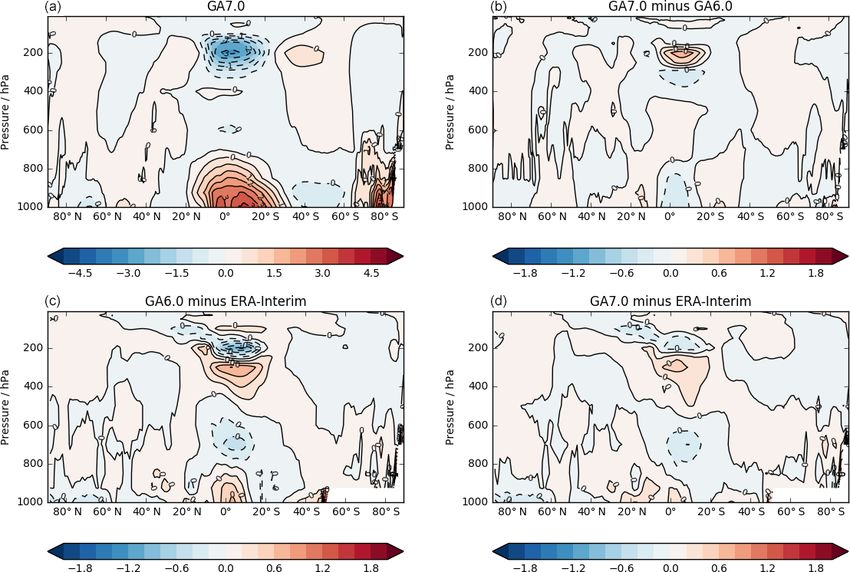
1918                                                                       D. Walters et al.: UM GA7.0/GA7.1 and JULES GL7.0 configurations

Table 3. Source datasets used to create standard ancillary files used in GA7.0/GL7.0.

   Ancillary field                                      Source data                                               Notes
   Land mask and fraction                               System dependent
   Mean and sub-grid orography                          GLOBE 3000 ; Hastings et al. (1999)                       Fields filtered before use
   Land usage                                           IGBP; Loveland et al. (2000)                              Mapped to nine tile types
   Soil properties                                      HWSD; Nachtergaele et al. (2008)                          Three datasets blended via optimal interpolation
                                                        STATSGO; Miller and White (1998)
                                                        ISRIC-WISE; Batjes (2009)
   Leaf area index                                      MODIS collection 5                                        4 km data (Samanta et al., 2012) mapped to five
                                                                                                                  plant types
   Plant canopy height                                  IGBP; Loveland et al. (2000)                              Derived from land usage and mapped to five plant
                                                                                                                  types
   Bare soil albedo                                     MODIS; Houldcroft et al. (2008)
   Snow-free surface albedo                             GlobAlbedo; Muller et al. (2012)                          Spatially complete white sky values
   TOPMODEL topographic index                           Marthews et al. (2015)
   SST and sea ice                                      System or experiment dependent
   Sea surface chlorophyll content                      GlobColour; Ford et al. (2012)
   Ozone                                                SPARC-II; Cionni et al. (2011)                            Zonal mean field useda
   GLOMAP-mode emissions and fields                                                                               Only required for
                                                                                                                  prognostic aerosol simulations
   Main primary emissions                               CMIP5; Lamarque et al. (2010)                             Includes SO2 , DMS (land), black carbon from
                                                                                                                  fossil fuel, organic carbon from fossil fuel
   Biomass burning                                      GFED3.1; van der Werf et al. (2010)                       10-year monthly means
   Volcanic SO2 emissions                               Andres and Kasgnoc (1998)
   Gas-phase aerosol precursors                         UKCA tropospheric chemistry simulations
                                                        O’Connor et al. (2014)
   Ocean DMS concentrations                             Kettle et al. (1999)
   CLASSIC aerosol climatologies                        System or experiment dependent                            Used when prognostic fields not available
   TRIP river paths                                     1◦ data from Oki and Sud (1998)                           Adjusted at coastlines to ensure correct outflow
 a This is expanded to a “zonally symmetric” 3-D field in limited-area simulations on a rotated pole grid.

the bias in lower-stratospheric water vapour by ≈ 50 %. This                                   3.1.2         Conservative advection of mass-weighted
change also improves the dynamical core’s internal consis-                                                   potential temperature (GA ticket #146)
tency as it means that we use the same three-dimensional
interpolation algorithms for temperature and moisture.                                         For an adiabatic flow, virtual dry potential temperature (θvd )
   For systems enforcing the mass conservation of moist                                        is constant within a fluid parcel moving with the flow. Ad-
prognostics (which we formally treat as a system-dependent                                     ditionally, the product of θvd and the density of dry air ρd is
option in the Global Atmosphere configuration) we change                                       also conserved, i.e.
the algorithm used from that described in Zerroukat (2010)
to the optimised conservative filter scheme (OCF; Zerroukat                                     ∂(ρd θvd )
                                                                                                           + ∇.(ρd θvd u) = 0.                                       (1)
and Allen, 2015). The OCF seeks to find a weighted con-                                            ∂t
servative solution between the high-order semi-Lagrangian
                                                                                               In the ENDGame formulation, however, the fluid flow is not
solution discussed above and a lower-order (trilinear) solu-
                                                                                               discretised in a conservative form; even in the absence of di-
tion, where the weights are optimised such that the conserva-
                                                                                               abatic sources and sinks, the semi-implicit semi-Lagrangian
tive solution stays as close as possible to the high-order one
                                                                                               time step does not satisfy the discrete form of Eq. (1),
whilst achieving conservation. This particular change has lit-
                                                                                               which leads to a spurious source of energy, as discussed in
tle impact on the moisture biases in the lower stratosphere
                                                                                               Sect. 5.4.3 of Walters et al. (2017).
but makes the conservation algorithm for moisture consis-
                                                                                                  In GA7, we address this by applying the same OCF
tent with that used for atmospheric composition fields (see
                                                                                               conservation-recovery algorithm discussed above in the con-
Sect. 3.8).
                                                                                               text of moist prognostics to the θvd field; unlike the con-
                                                                                               servation of moist prognostics, however, this is not treated
                                                                                               as a system-dependent option and is applied in all systems
                                                                                               using GA7. This improves the warm biases in the tropical
                                                                                               tropopause layer, as discussed in Hardiman et al. (2015). By
                                                                                               removing this spurious source of energy, it also reduces the

Geosci. Model Dev., 12, 1909–1963, 2019                                                                               www.geosci-model-dev.net/12/1909/2019/
D. Walters et al.: UM GA7.0/GA7.1 and JULES GL7.0 configurations 1919
size of (and resolution dependence in) the global energy cor- The resulting SW treatment improves the representation of
rection step used in long climate simulations, as described H2 O, CO2 , O3 , and O2 absorption compared to GA6 and also
in Sect. 2.13. now includes absorption from N2 O and CH4 . Changes re-
sult in increased atmospheric absorption and reduced surface
3.1.3 Reduction of solver tolerance in the iterative (clear-sky) fluxes reducing errors compared to reference re-
Helmholtz solver (GA ticket #153) sults from the Continual Intercomparison of Radiation Codes
(CIRC; Oreopoulos et al., 2012).
As discussed in Sect. 2.1 and 2.2, an important part of the The new LW treatment improves the representation of all
ENDGame time step is the iterative solution of the lin- gases resulting in reduced clear-sky outgoing LW radiation
ear Helmholtz problem to determine the model’s pressure (OLR) and increased downward surface flux. In particular,
field. The approach is said to have reached its solution when improvements to the treatment of the water vapour contin-
a global normalised residual term (the solver “norm”) is uum significantly improve the downward LW surface fluxes
smaller than a predetermined small value, or “tolerance”. The in regions of low humidity. The stratospheric heating rates, in
smaller the tolerance, the more accurate the solution, albeit particular the stratospheric water vapour forcing, are signif-
at the cost of requiring more iterations to reach it. In GA6, icantly improved, addressing errors described by Maycock
the solver tolerance was set to 1 × 10⁻³ , which was thought and Shine (2012). There is also a significant improvement
a suitable balance between accuracy and computational cost. in the CO2 forcing, especially for CO2 concentrations of 4
At horizontal resolutions at or above about N512 (≈ 25 km times the present-day value and above. Figure 1 compares the
in the mid-latitudes), however, global GA6 simulations suf- errors in LW fluxes for various CO2 concentrations based on
fered from numerical noise in the meridional wind near the the clear-sky atmospheric profiles used for CIRC. In both the
poles in the topmost few levels (i.e. at altitudes of 65 km and SW and LW regions there is a significant improvement in the
above). The underlying cause of this noise is not known, but band-by-band breakdown of absorption compared to GA6
it was noted that local calculations of the solver norms have where cancellation of errors between different bands was im-
shown that these are largest close to the poles. Although the portant. This should improve the interaction with band-by-
cause and effect is unclear, reducing the global solver toler- band aerosol, cloud, and surface properties such as the albedo
ance by 2 orders of magnitude makes the noise almost im- of the sea.
perceptible, but this is at the cost of increasing model run
time by over 50 %. Reducing by only a single order of mag- 3.2.2 Improved treatment of sub-grid-scale cloud
nitude, however, significantly reduces this noise, whilst only water content variability (GA ticket #15)
increasing run time by ≈ 15 %. For this reason, in GA7 we
have implemented this compromise and use a solver toler- In order to represent the radiative effects of sub-grid-scale
ance of 1 × 10⁻⁴ . water content variability, the radiation scheme uses the
McICA as described in Hill et al. (2011). In the McICA,
3.2 Solar and terrestrial radiation the variability of water content within a grid box is deter-
mined by a fractional standard deviation (f ), which is equal
3.2.1 Improved treatment of gaseous absorption (GA to the standard deviation of cloud water content in a grid
ticket #16) box divided by its mean value. The transmission of radiation
through a cloud is a convex function of the cloud water con-
GA7 includes an updated treatment of gas absorption with
tent such that increasing the value of f decreases the radia-
newly derived correlated-k coefficients for all gases as de-
tive effect of a cloud, whilst decreasing f has the opposite ef-
scribed in Sect. 2.3. Generation and validation of the gas
fect (e.g. Shonk and Hogan, 2010). In GA6, we used a glob-
absorption coefficients involved the creation of two con-
ally constant value of f = 0.75, but in reality, the water con-
figurations: a high wavelength resolution reference config-
tent variability itself is variable and the magnitude of f has
uration (for offline comparison and diagnostic use) and a
been linked to cloud type, cloud fraction, wind shear and do-
low-resolution broadband configuration for use in the full
main size (e.g. Hogan and Illingworth, 2003; Oreopoulos and
model. The reference configurations contain 300 bands in
Cahalan, 2005; Hill et al., 2012). At GA7, we include some
the LW and 260 bands in the SW (SOCRATES spectral
of these effects by determining f from the parametrisation
files: sp_lw_300_jm2, sp_sw_260_jm2) and are based on the
of P. G. Hill et al. (2015). In the interests of physical consis-
same data sources as the broadband files (primarily HITRAN
tency, this parametrisation is also used in the warm rain part
2012). These were validated against independent line-by-line
of the microphysics scheme. The implementation of the P.
codes and were subsequently used as a reference to verify the
G. Hill et al. (2015) parametrisation results in f that depends
performance of the broadband configurations (SOCRATES
on cloud fraction, vertical layer thickness, and whether or not
spectral files: sp_lw_ga7, sp_sw_ga7) over a range of atmo-
the cloud is convective, where convective cloud is identified
spheric conditions and greenhouse gas forcing scenarios.
based on the activation of the convection scheme.
www.geosci-model-dev.net/12/1909/2019/ Geosci. Model Dev., 12, 1909–1963, 2019You can also read