Pricing Characteristics in the German Diesel Retail Market after the Introduction of the Market Transparency Unit
←
→
Page content transcription
If your browser does not render page correctly, please read the page content below
Current and Future Challenges to Energy Security
           2nd AIEE Energy Symposium, Rome, Italy

          Pricing Characteristics in the
German Diesel Retail Market after the Introduction
       of the Market Transparency Unit

         Sebastian Kreuz, Chair of Energy Economics,
        University of Technology in Cottbus, Germany

                      Rome, 3rd November 2017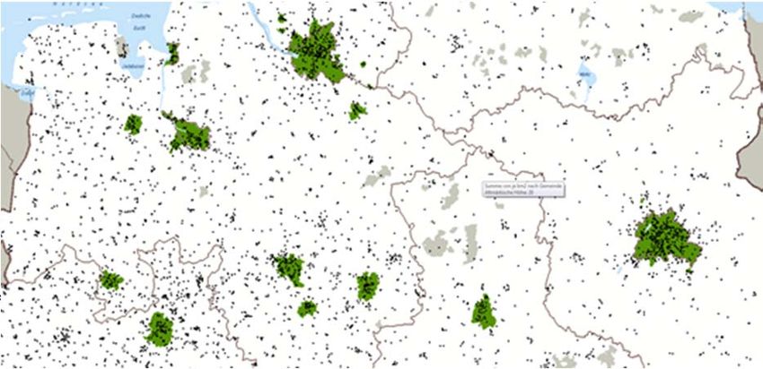
Agenda
Introduction
Data
Research Questions
Methods:
– Asymmetric Error Correction Model
– Semi‐Asymmetric Error Correction Model
Results
Further Research
2
Introduction
High public relevance of gasoline price
development
Long tradition of research concerning
relationship of gasoline and oil prices, e. g.
Rockets and Feathers (Asymmetric Price
Transmission) “Rockets and Feathers are
given when fuel prices increase faster than
they decrease after oil price changes. ”
Widely discussed questions:
– Do retailers increase prices faster with
increasing oil prices?
– Is market power given?
3
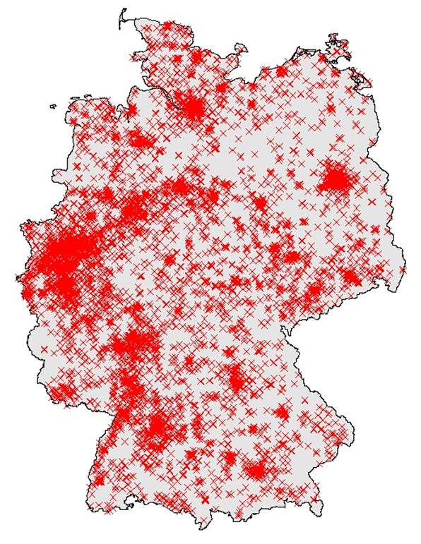
Data (1): Market Transparency Unit in Germany
Data set was gathered from an online platform via the market
transparency unit
Part of the german Federal Cartel Office;
established to increase market transparency on the retail market
“Since […] 2013 companies which operate public petrol stations […] are
obliged to report price changes […] of fuel […] in real time“
4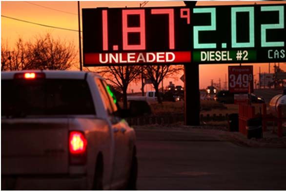
Data (2): Diesel Data
In total: More than 20 million prices for all german fuel stations
Daily prices for the period from June 2014 to May 2016 of about 6800 retail fuel
stations highly disaggregated data
The database enables to differentiate between brands and regions
5Research Questions
1. Do diesel prices follow oil prices in the long‐run (cointegration)?
2. Do major brands (Shell, Total, Jet, Esso, Aral) show different pricing
characteristics concerning asymmetry than all other stations?
3. Do independent petrol stations show different pricing characteristics
concerning asymmetry than all other stations?
4. Do petrol stations in lower populated regions (PopDens low) behave
differently concerning asymmetry from stations in more urban areas
(PopDens high)?
– Threshold: 1000 inhabitants/km²
6Methods (1a): Creating the Asymmetric Error Correction
Model following Engle/Granger
Test for stationarity (ADF‐Test) of fuel ∆ , , , ∆
and oil in levels and in first differences
Results need to show that the data is
integrated on the same scale of ∆ , , ∆
integration.
a) OLS: Estimate the cointegration relationship
: , , and testing residuals for stationarity
b) Using the residuals within the Error
Correction Model
,
Estimate asymmetric ∆ , ,, ∆ ,, ∆ ,, ∆ ,, ∆
error correction
model: threshold
variable for ∧ 0 0, ∧ 0 0;
decomposing , ∆ ∆ ∆ ∧∆ 0 ∆ 0, ∆ ∆ ∧∆ 0 ∆ 0; ∆ ∆ ∧∆
and ∆ is zero; 0 ∆ 0, ∆ ∆ ∧∆ 0 ∆ 0
7Methods (1b): Interpretation of model results
∆ , , , ∆ , , ∆ , , ∆ , , ∆
Testing for speed back into
the long-term equlibrium
Positive error term: real diesel price is higher than equilibrium price Rockets and
feathers: this reversion should be slower.
Negative error term: real diesel price is lower than equilibrium price Rockets and
feathers: this reversion should be faster.
Testing for difference between and (Wald‐test) H 0 : and
H1:
8Methods (2a): Creating the Semi‐Asymmetric Error Correction
Model following Engle/Granger
Test for stationarity (ADF‐Test) of fuel ∆ , , , ∆
and oil in levels and in first differences
Results need to show that the data is
integrated on the same scale of ∆ , , ∆
integration.
a) OLS: Estimate the cointegration relationship
: , , and testing residuals for stationarity
b) Using the residuals within the Error
Correction Model
,
∆ , ,, ∆ ,, ∆
Estimate semi‐asymmetric error
correction model: Threshold variable
for decomposing is sign of the mean where
of wholesale oil price changes ∆ 1 1
over lags (number of lags from ∧ 0, ∆ 0, ∧ 0, ∆ 0,
optimal OLS)
∆
9Methods (2b): Interpretation of model results
∆ , ,, ∆ ,, ∆
Testing for speed back into
the long-term equlibrium
But with different interpretation: Are coefficients ? faster
adjustment for increasing oil prices
Testing for difference between and (Wald‐test) H 0 : and
H1:
10Current Results
1. Test for order of cointegration
2. Cointegration
3. ECM
a. Asymmetric ECM (A‐ECM)
b. Semi‐Asymmetric ECM (SA‐ECM)
11Current Results (1): Cointegration
Share [%]; Share [%];
Cointegration-Model – lag
significance significance
selection by BIC
level 1 % level 5 %
OLS max. 7 lags 85 % 96 %
OLS max. 10 lags 79 % 94 %
OLS max. 14 lags 79 % 94%
12Current Results (2): Asymmetric and Semi‐Asymmetric ECM for
all cointegrated retail stations
Wald‐Test: 10 % Significance level
Cases/Scenarios/Data A‐ECM (BIC) SA‐ECM (BIC)
Rockets and Feathers Asymmetry 16.87% 10.74%
Brand Asymmetry 19.77% 14.27%
Non‐Brand Asymmetry 12.52% 5.43%
Independent Asymmetry 12.11% 4.41%
Non‐Independent Asymmetry 17.31% 11.32%
PopDens high Asymmetry 12.55% 9.64%
PopDens low Asymmetry 18.26% 11.09%
Comparable results for
– different significance levels of the Wald‐Test (5 % significance level),
– DOLS cointegration relationship instead of OLS and
– AIC as lag selection indicator instead of the BIC
13Further Research
Further models…
Model improvements…
Model testing…
Displaying results…
14“Pricing Characteristics in the German Diesel Retail Market
after the Introduction of the Market Transparency Unit”
Thank you very much for your attention.
Dipl.‐Vw. Sebastian Kreuz
Research Assistant, PhD candidate
Chair of Energy Economics, Brandenburg University of Technology Cottbus‐
Senftenberg
Sebastian.Kreuz@b‐tu.de
https://www.b‐tu.de/en/fg‐energiewirtschaft
15Test for Stationarity, Cointegration and Error Correction Model
In practical analytical work stationarity of a time series means
regression with lags
– no trend
– no systematic change of variance
– no strictly periodic fluctuations
– no systematically changing interdependencies between the elements of the time
series
Cointegration tries to investigate long-term relationships between non-
stationary variables
ECM (with non-stationary variables): tries to estimate the parameters of
the long-term and short-term relationship between both (cointegrated)
variables
16Conclusion
About 80 % of fuel station have very strong cointegration relationships
with wholesale oil prices
About 11 % to 16 % of these fuel stations show characteristics of
asymmetry like Rockets and Feathers
There seem to be higher shares of asymmetric price responses to oil price
changes for mayor brands, non‐independent fuel stations and fuel
stations in regions with lower population densities
17Current Results (1): Cointegration
Share [%]; Share [%];
Cointegration-Model – lag selection by BIC
significance level 1 % significance level 5 %
OLS max. 7 lags 85.20% 96.10%
OLS max. 10 lags 79.37% 93.49%
OLS max. 14 lags 79.41% 94.01%
DOLS max. 7 lags 85.67% 96.32%
DOLS max. 10 lags 82.08% 95.26%
DOLS max. 14 lags 80.28% 94.35%
1819
Methods (1a): Creating the Asymmetric Error Correction
Model following Engle/Granger
Test for stationarity (ADF‐Test) of fuel ∆ , , , , ∆
and oil in levels and in first differences
Results need to show that the data is
integrated on the same scale of ∆ , , ∆
integration.
: a) (D)OLS: Estimate the cointegration
, ,
relationship iesel ~ oil and testing residuals
for stationarity
: , , ,, ∆ b) Using the residuals within the Error
Correction Model
Estimate asymmetric ∆ , ,, ∆ ,, ∆ ,, ∆ ,, ∆
error correction
model: threshold
∧ 0 0, ∧ 0 0;
variable for ∆ ∆ ∧∆ 0 ∆ 0, ∆ ∆ ∧∆ 0 ∆ 0; ∆ ∆ ∧∆
decomposing , ∆ 0 ∆ 0, ∆ ∆ ∧∆ 0 ∆ 0
and ∆ is zero;
20Methods (2a): Creating the Semi‐Asymmetric Error Correction
Model following Engle/Granger
Test for stationarity (ADF‐Test) of fuel ∆ ∆
, , , ,
and oil in levels and in first differences
Results need to show that the data is
integrated on the same scale of ∆ , , ∆
integration.
: a) (D)OLS: Estimate the cointegration
, ,
relationship diesel ~ oil and testing
residuals for stationarity
: , , ,, ∆ b) Using the residuals within the Error
Correction Model
∆ , ,, ∆ ,, ∆
Estimate asymmetric error correction
model: Threshold variable for
decomposing is sign of the mean of where
wholesale oil price changes ∆ 1 1
over lags (number of lags from ∧ 0, ∆ 0, ∧ 0, ∆ 0,
optimal ((D)OLS) ∆
21You can also read