The Role of COVID-19 in Spatial Reorganization: Some Evidence from Germany - HWWI Research
←
→
Page content transcription
If your browser does not render page correctly, please read the page content below
The Role of COVID-19 in Spatial
                    Reorganization: Some Evidence
                    from Germany
                    Andree Ehlert, Jan Wedemeier, Tabea Zahlmann

HWWI Research
        Paper 195

                    Hamburg Institute of International Economics (HWWI) | 2021
                    ISSN 1861-504X
Contact:
Dr. Jan Wedemeier
Hamburg Institute of International Economics (HWWI)
Fahrenheitstr. 1 | 28359 Bremen | Germany
Phone: +49 (0)421 2208-243 | Fax: +49 (0)40 340576-150
wedemeier@hwwi.org

Prof. Dr. Andree Ehlert
Harz University of Applied Sciences
Faculty of Business Studies
Friedrichstr. 57 - 59 | 38855 Wernigerode | Germany
aehlert@hs-harz.de

HWWI Research Paper
Hamburg Institute of International Economics (HWWI)
Oberhafenstr. 1 | 20097 Hamburg, Germany
Telephone: +49 (0)40 340576-0 | Fax: +49 (0)40 340576-150
info@hwwi.org | www.hwwi.org
ISSN 1861-504X

Editorial board:
Prof. Dr. Henning Vöpel

© by the authors | May 2021
The authors are solely responsible for the contents which do not
necessarily represent the opinion of the HWWI.
HWWI Research Paper 195

The Role of COVID-19 in Spatial Reorgani-
zation: Some Evidence from Germany
Andree Ehlert, Jan Wedemeier, Tabea Zahlmann

Abstract This paper analyzes the role of regional demographic, socioeconomic and po-
litical factors on changes in mobility during the COVID-19 pandemic. It provides new
empirical evidence for the regional differentiation of lockdown measures and indicates
a possible reorganization of spatial economic and social activities beyond the course of
the pandemic. Spatial econometric models are analyzed using data from the 401 counties
in Germany. Our results show that, for example, current high caseloads are negatively
related to changes in mobility, whereas a region’s socioeconomic composition and rural
location have a positive effect. The political and economic implications of the findings
are discussed.

Key words Economic geography, COVID-19 pandemic, lockdown, regional interaction,
mobility, spatial econometrics

JEL R10, R11, R12

                                                                                       1
1 | Introduction
The COVID-19 pandemic is a major societal and economic challenge, with 152 million
infections and 3.2 million deaths worldwide (as of May 2, 2021). Policymakers are re-
sponding with a wide variety of instruments, including in Germany: temporary closures
of businesses, especially in the arts, entertainment and recreation, or hospitality sectors,
suspension of compulsory attendance at schools, and repeated requests to increase use
of home office options. In addition to restricting contacts, these measures also have the
simultaneous effect of limiting mobility. In Germany, measures to restrict contacts were
implemented for the first time in March 2020. Examples include direct mobility re-
strictions such as certain km radii around the place of residence, temporary entry re-
strictions to certain federal states or counties (Kreise), and (nighttime) curfews. Indirect
mobility restrictions consist of repeated appeals to the population to avoid private and
tourist travel, the closure of restaurants, cafés and leisure facilities and, eventually, self-
motivation (caution and insight) to refrain from contacts and travel. From an economic
point of view, therefore, a bundle of measures has increased the individual costs of mo-
bility and, at the same time, reduced its attractiveness (utility).
How does mobility change in response to high infection rates and corresponding po-
litical measures? And on what other factors besides these measures and (possibly deter-
rent) COVID-19 case and death rates does this change in mobility depend? While mobil-
ity changes in times of the COVID-19 pandemic have been extensively analyzed in the
literature at the individual, regional, or economy-wide level, this study asks two previ-
ously unanswered questions: First, what are the specific factors influencing mobility
change in a regional context? In other words: What socioeconomic, geographic, and
health factors are associated with changing mobility in the wake of the pandemic? Sec-
ond, the question of spatial spillover effects of the mobility change per se arises. From a
statistical perspective not considering these spatial interactions could bias the answer to
our first question. Further, the spillover effects themselves are also of economic interest.
This raises, for example, the question of learning effects from neighboring regions (pos-
itive spillover effects, "if mobility is reduced there, then we should reduce it here, too"),
but also the opposite question of possible spatial substitution of mobility, i.e., whether
the reduction of mobility in one county is replaced by an increase of mobility in the
neighboring counties (negative spillover effects, "if the kin do not come to me, then I will
just come to my kin").
2These questions have far-reaching economic and political relevance. On the one hand,
they can expand the still limited knowledge on the heterogeneous effectiveness of lock-
down measures. Related to this is the question of deriving, for example, region-specific
and thus more targeted measures than before, if it is known how which socioeconomic
factors constrain or promote mobility change in the wake of COVID-19. In addition, the
long-term, potentially spatially transformative effects are of particular interest (cf. Sec-
tion 2).
Demographic, socioeconomic, and meteorological data as well as data on political
COVID-19 measures (also at the county level) from various sources are used as covari-
ates. These are supplemented by the regional COVID-19 case numbers provided by the
Robert Koch Institute (RKI). Note that this study is based on the analysis of aggregated
data (ecological study) with the associated limitations in terms of interpretation of the
results, which also should be limited to the region level. A direct application of the re-
sults to the individual level can lead to so-called ecological fallacies, for which there are
numerous examples in the literature. However, this only conditionally limits the rele-
vance of our results, since the lockdown (and other policy) measures in question are also
discussed solely at the regional level. The data are analyzed using the spatial autoregres-
sive combined model (SAC). The location of the regions with respect to each other is
captured by a weighting matrix. Note that these spatial models can reduce potential bias
of ordinary least squares (OLS) estimation in the case of spatial spillovers and/or increase
estimation efficiency.
The paper expands the existing literature on the spatial impact of COVID-19 in rela-
tion to several aspects. Schlosser et al. (2020) study the influence of the pandemic on the
mobility of individuals. The authors stress that the pandemic has substantial influence
on the mobility. They find that especially long-distance travel has been reduced strongly.
Koenig and Dressler (2021) present results of a mixed-methods analysis of mobility
changes in a German rural area. Their study analyses mobility data and survey data on
the perceived changes of people based on a representative household survey. Linka et
al. (2021) investigate the dynamics between mobility and COVID-19 operationalized by
global air traffic and local mobility. Their study demonstrates different intensities of dis-
ease dynamics. For ten European countries there is a time lag between mobility and dis-
ease dynamics of around 14.6 days on average. Other examples of extant literature in-
clude Coven and Gupta (2020) or Bludau et al. (2020).
The paper is structured as follows. A brief overview of spatial theory is given in Sec-
tion 2. The data used and the statistical methodology are presented in Section 3. A dis-
cussion of the empirical results follows in Section 4. Section 5 then relates these results
to their spatial implications. Section 6 concludes.
32 | Theory of Spatial Structure
The spatial distribution of economic activities has been discussed in the principles of
the classical theory of location such as von Thünen (1826), Weber (1909), or Lösch (1944)
– just to mention a few. In general, economic and social development always have a
spatial dimension. This importance is reflected in regional peculiarities, in differences in
economic activities, or living conditions (Bröcker and Fritsch 2012). Spatial activity – and
thus prosperity and economic action – is unevenly distributed. Exogenous and endoge-
nous explanations can help to explain this fact.
The exogenous explanation takes the geographical conditions as given, companies
and households adapt their behavior accordingly. There are also other characteristics
that can be traced back to economic decisions, such as the locations of (supply) markets.
Moreover, the endogenous explanations are reasons for a differentiated, unevenly dis-
tributed spatial structure of economic activities in a homogeneous area (without geo-
graphical differences). In addition to many differentiated approaches, the spatial costs
are the basis of the geographic economy. Costs to overcome spatial distance must be
lower than the benefits of an interaction (taking complementarity and no alternative op-
portunity costs into account). It can be plausibly assumed that spatial costs during a
pandemic are higher for individuals (for a given technology). The benefits of home office
are possibly greater than that of the open shared office. Avoiding public transport or
other modes of transport increases benefits of organizing work at home.
The space overcoming costs arise when households and companies move goods, peo-
ple and information in space. In addition to transport costs, we refer to all costs for over-
coming space, including costs for transmitting communication. It is crucial that these
costs have fallen massively in recent years in order to move goods, people and infor-
mation through space over distances – sometimes around the globe. But these costs are
still relevant. However, it should also be noted that although the transaction costs are
steadily falling during the exchange, more information is exchanged – and this also over
greater distances – than ever before (Bröcker and Fritsch, 2012).
The triggers for spatial differentiation – the juxtaposition of growing cities, metropol-
itan regions, and shrinking regions – are the interdependent location decisions of work-
ers and companies. Ongoing globalization, the European integration process and tech-
nological progress – especially in the field of IT – have led to a continuous decline in
transport and communication costs. This development facilitates the mobility of labor
and capital, the dissemination of information, and the exchange of goods and services
between regions. But, it also helps to reduce the costs of communication between
4employees of the same company, customers, and clients (e.g. virtual conference and
meetings). The location ties of production factors and workers, but also families, have
decreased. On average, companies settle where they find the most attractive location
conditions. Workers and their families are migrating to regions that offer them attractive
working and living conditions. Regions are permanently in intense competition for com-
panies and qualified workers.
The question is how stable this equilibrium is and whether the framework will shift
as a result of the pandemic and thus massively reduce the costs to overcome space
through the intensively use of digital solutions.
3 | Data and Methods
3.1 | The Data
This analysis is a retrospective ecological study at the level of 401 counties (Kreise) in
Germany, whose populations range from about 34,000 (Zweibrücken) to about 3,664,000
(Berlin). As an outcome variable, the study uses the change in general mobility behavior
at the county level in January 2021 (average values are calculated separately for week-
days and weekends for the entire month from January 4 to exclude the influence of the
New Year's weekend) compared to the same period of the previous year. The mobility
data are provided by the Federal Statistical Office (2021). To map mobility at the district
level, anonymized mobile communications data from the network of the communica-
tions provider Telefónica (Germany-wide market share ≥ 30%) are used, which are pro-
cessed and made available by Teralytics. The data provides an overview of the number
of mobile devices performing a certain movement. Movements are recorded when a mo-
bile device changes the cell. The target region of a movement is reached when the mobile
remains in a cell for at least 30 minutes. Deviations in relation to the total population
may occur due to the provider's regional market shares, which are, however, partially
compensated for by the provider using an algorithm based on geographic differentiated
market shares. 1
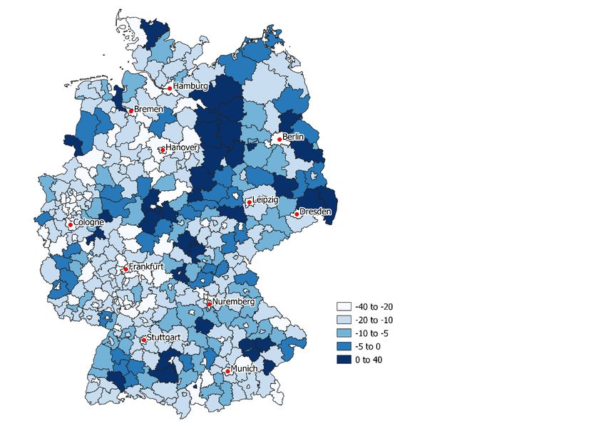
As a target variable for the analysis, data provided by the Federal Statistical Office on
mobility change between January 2021 and January 2020 are analyzed at the county level
(cf. Fig. 1). Note that a decline in mobility was observed in most of the regions. However,
1 See https://www.destatis.de/DE/Service/EXDAT/Datensaetze/mobilitaetsindikatoren-mobilfunkdaten.html for details.
5the former border areas between Lower Saxony on the one hand and Saxony-Anhalt and
Brandenburg on the other show increased mobility. The month of January 2021 was cho-
sen as the core period of the second COVID-19 wave in Germany. In addition, the same
month of the previous year, January 2020, was the month before the pandemic hit Ger-
many (and the rest of the global economy).
In addition to the COVID-19 case numbers provided by the RKI at the county level,
various socioeconomic, demographic, meteorological, political and health variables (in-
cluding government restrictions on mobility) at the county level are used as covariates
whose possible influence on (COVID-19-related) mobility change will be analyzed. An
overview is provided in Table 1.
Figure 1: Mobility change on working days (Jan 2021 vs. Jan 2020) at county level
Source: infas 360 (2021).
6Table 1: Basic sample characteristics
Variable Mean Median SD N
Change in mobility in %. -13.274 -13.250 10.953 401
Cases Jan 2021 (per 100,000 inhabitants) 590.342 512.592 281.252 401
Cases Dec 2020 (per 100,000 inhabitants) 822.709 750.256 414.382 401
Deaths Jan 2021 (per 100,000 inhabitants) 23.144 18.502 17.550 401
Deats Dec 2020 (per 100,000 inhabitants) 31.669 24.733 25.020 401
Unemployment rate 2020 5.487 5.200 2.198 401
Unemployment rate Jan. 2021 5.908 5.600 2.215 401
Household income 1,872.561 1,869.000 215.765 401
Nursing home employees 97.709 96.800 23.279 401
Share of employed academics 11.958 10.300 5.170 401
Industry share 18.254 17.200 8.724 401
Service share 39.243 33.900 14.842 401
Tourist beds 41.776 27.000 49.309 401
Mean age 44.539 44.300 1.965 401
Women 50.597 50.600 0.645 401
Heart failure 3.845 3.530 1.420 401
COPD 6.455 6.400 1.503 401
Physicians 14.587 12.900 4.409 401
Pharmacies 27.004 26.100 4.900 401
People in need of care 428.125 424.200 106.029 401
Population density 533.748 198.000 702.713 401
Car density 579.160 593.000 70.980 401
Commuter balance -10.362 -12.000 29.724 401
Share of foreigners 10.035 9.200 5.149 401
Rural (0/1) 0.339 0.000 0.474 401
Pupils 10.125 10.000 1.501 401
Childcare 32.269 28.800 12.077 401
Car travel time central city (Mittelzentrum) 6.786 8.000 5.548 401
Commute over 300km 2.402 2.200 0.892 401
In selecting the possible factors influencing mobility change, we largely followed the
existing literature and the following substantive arguments:
− Case numbers previous month: People remember infection events, align their
behavior accordingly with a time lag.
− Deaths: It can be assumed that the deterrent effect (also in the media) is partic-
ularly large.
− Unemployment rate: This has both direct (fewer trips to work) and indirect
effects (search activities, less financial scope for trips) on mobility.
− Household income: The level of income is correlated with job and place of res-
idence. When analyzing the modal shift, Koenig and Dressler (2021) showed
7that the number of car trips is significantly associated with a higher net house-
hold income.
− Nursing home employees: It is of particular interest whether there is leeway in
outpatient care to restrict mobility.
− Employment/industry structure: It is expected that home office will be more
feasible for employees in the service than in the industry sector. Therefore, re-
gions with a high industrial share will presumably be less affected by a decline
in mobility.
− Health variables: Several studies suggest that pre-existing conditions includ-
ing hypertension, lung diseases, respiratory diseases and heart failures signif-
icantly increase the risk of a severe course of a COVID-19 infection or death
(Guan et al. 2020; Guo et al. 2020; Ssentongo et al. 2020). Due to the wide dis-
closure of those research results people with such pre-existing conditions are
more likely to decrease their mobility.
− Demographic variables: Demographic variables (mean age, woman, share of
foreigners) are relevant in the context of employment and mobility. In Ger-
many, for example, due to the pandemic, the unemployment rate for men
(from 5.3% to 6.7%) increased slightly more than that of women (from 4.9% to
5.9%). At the same time, foreigners (from 12.1% to 15.5%) are much more af-
fected than Germans (from 4.1% to 5.1%) (reference month July 2019 and July
2020) (Nitt-Drießelmann et al. 2020). Due to the higher proportion of foreigners
among the low and medium-skilled employees, it may be expected that mo-
bility among this group will decrease less sharply.
3.2 | Methods
What influences the COVID-19-related change in mobility at the county level and how
can the influence of non-COVID-19-related circumstances be at least partially accounted
for? Since this research is forced to be a historically controlled study, the question of
changed concomitant circumstances that would have varied on an annual basis even in
the absence of the COVID-19 pandemic and thus cannot be attributed to the pandemic
must be carefully considered. The potential bias will be only partially avoidable from a
statistical perspective but will be mitigated by the comprehensive covariates (variance
in area, i.e., their possible influence on the changed accompanying and living circum-
stances). Conceivable biasing factors include general trends in regional mobility, holiday
effects, and the influence of weather on mobility (e.g., for excursions). The last point is
taken into account by the separate analysis of weekdays and weekends, as well as the
8inclusion of differences in sunshine duration and temperature between January 2021 vs.
2020 (whereby mobility in the month of January is certainly less influenced in this respect
than in the summer months, so that some general robustness can be assumed for the
study period). Furthermore, holiday effects are already taken into account in the data
preparation by the Federal Statistical Office (2021). General trends in mobility over time
are accounted for, at least indirectly, by its relation to socioeconomic variables and, of
course, by the inclusion of a constant term.
Taking the above constraints into account, our identification strategy works as fol-
lows. We assume that the mobility change is driven, on the one hand, directly by contact
and mobility restriction policies such as, in particular, contact restrictions in public
space, wholesale and retail restrictions, restrictions in the tourism sector, and curfews.
Our corresponding variables (see Table 1) reflect whether or not these restrictions were
in effect on a given day in January 2021. On the other hand, we assume that mobility
change is driven indirectly by the COVID-19 case numbers (e.g. people adjust their life-
style after being repeatedly encouraged to do so by policy makers) in addition to the
above policy measures. We thus assume that regional heterogeneity of case numbers
serves as a central COVID-19-related parameter influencing mobility. We also test the
additional hypothesis that not only COVID-19 case numbers have an impact on mobility,
but that this impact is moderated by socioeconomic covariates (interaction effects).
In contrast to a standard linear model (OLS), our analysis takes into account the spatial
distance of the observation units (counties) from each other. Spatial statistical models
(see below) are then able to reflect the fact that outcomes in one region may be influenced
by outcomes in neighboring regions (spatial spillover effects) and/or a spatial autocorre-
lation of the residuals. This proposition can be explained, e.g., via learning effects from
neighboring regions or, in contrast, spatial substitution of mobility. In the latter case re-
duced mobility in one region is quasi-substituted by increased mobility in neighboring
regions, see the discussion in Section 1.
The spatial statistical models capture the neighborhood relationships using a so-called
spatial weighting matrix (i.e., a symmetric N×N matrix). This is based here on the geo-
codes (longitude and latitude of the circle centers) provided by the provider
Opendatasoft (under the Creative Commons license). Specifically, the spmatrix com-
mand in Stata/MP 16.1 was used to create an inverse distance matrix from the coordi-
nates, in which regions closer to each other are given a higher weight. The technical de-
tails of the spatial statistical models shall be omitted here with reference to the detailed
discussion in Elhorst (2014).
94 | Results
The data analysis was performed using the spregress command in Stata/MP 16.1. Ta-
ble 2 shows the results for the SAC model, which we focus on here, because it includes
the spatial autoregressive and spatial error models as special cases. 2 Before discussing
the individual coefficient estimators, we briefly note the LR test vs. the OLS model at the
bottom of the table. This does not support the use of a spatial SAC model because the
null hypothesis of an OLS model cannot be rejected.
Table 2 contains results for the change in mobility on weekdays (January 2021 versus
January 2020) in the left-hand three-column block and results for weekends (in January
2021 versus January 2020, excluding the New Year's weekend) in the right-hand block.
In each case, the coefficient estimators, standard errors, and p-values are given. Dum-
mies for the 16 states were included (not shown) in the estimation to account for the
influences of state-specific COVID-19 measures (for which no reliable database is avail-
able).
Starting with the estimation results for weekdays, the significant negative association
between the average (population-standardized) case numbers in January 2021 and the
mobility change can be noted first. Both the previous month's caseload and death rates
show no significant association with changes in mobility behavior, disproving the (time-
lagged) deterrent effect hypothesis discussed in Section 3.1. The unemployment rate
shows a time-delayed effect reversal. The average unemployment rate in the previous
year has a significantly positive impact on mobility behavior, while the contemporane-
ous unemployment rate in January 2021 has a significantly negative impact. On the one
hand, a time-delayed higher mobility due to the search activities for a new job can be
discussed as an explanation. Note that with regard to the negative coefficient of January
2021 unemployment, endogeneity cannot be ruled out either, as (forced) reduced mobil-
ity can also have simultaneous negative effects on the labor market. The share of gradu-
ates and the share of service providers clearly show a significant negative association
with changes in mobility. This can be explained in particular by the higher home office
rates in service occupations, which often require a higher level of education.
2 The results for the latter two models are not reported, but are very similar to those in Table 2.
10Table 2: Estimation results
(Dummy variables for the federal states were included, results not shown).
Weekdays Weekends
Coefficient estimates Coef. Std. Err. P>|z| Coef. Std. Err. P>|z|
Cases Jan 2021 (per 100,000 inhabitants) -0.009 0.004 0.016 -0.009 0.004 0.028
Cases Dec 2020 (per 100,000 inhabitants) -0.003 0.002 0.268 -0.003 0.003 0.264
Deaths Jan 2021 (per 100,000 inhabitants) 0.062 0.040 0.127 0.059 0.047 0.212
Deats Dec 2020 (per 100,000 inhabitants) 0.024 0.032 0.447 0.022 0.037 0.561
Unemployment rate 2020 4.522 1.995 0.023 5.160 2.328 0.027
Unemployment rate Jan. 2021 -4.342 1.897 0.022 -4.643 2.213 0.036
Household income 0.005 0.003 0.127 0.007 0.004 0.067
Nursing home employees 0.027 0.026 0.308 0.033 0.031 0.278
Share of employed academics -0.512 0.164 0.002 -0.043 0.191 0.823
Industry share -0.017 0.068 0.805 0.034 0.079 0.671
Service share -0.206 0.075 0.006 -0.232 0.087 0.007
Tourist beds -0.002 0.011 0.868 -0.008 0.013 0.513
Mean age 1.033 0.545 0.058 1.213 0.638 0.057
Women -1.293 0.856 0.131 -1.801 0.992 0.069
Heart failure 0.201 0.483 0.678 0.423 0.569 0.457
COPD -0.937 0.401 0.019 -1.164 0.470 0.013
Physicians -0.166 0.233 0.477 0.110 0.271 0.686
Pharmacies -0.199 0.122 0.102 -0.276 0.142 0.052
People in need of care 0.020 0.008 0.014 0.031 0.009 0.001
Population density -0.001 0.001 0.387 -0.001 0.002 0.349
Car density -0.021 0.012 0.073 -0.028 0.013 0.039
Commuter balance 0.024 0.032 0.450 -0.004 0.038 0.924
Share of foreigners 0.461 0.186 0.013 0.276 0.218 0.206
Rural (0/1) 2.598 1.084 0.017 1.368 1.282 0.286
Pupils -0.366 0.380 0.335 0.041 0.435 0.924
Childcare 0.082 0.101 0.414 0.091 0.117 0.436
Car travel time central city (Mittelzentrum) -0.227 0.124 0.067 -0.129 0.144 0.372
Broadband coverage -0.082 0.043 0.059 -0.121 0.050 0.017
Commute over 300km -1.555 0.753 0.039 -1.855 0.882 0.035
Diff. hours of sunshine -0.032 0.041 0.438 -0.021 0.048 0.670
Diff. temperature 1.462 1.451 0.314 0.165 1.723 0.923
Contact restrictions in public space (0/1) 5.347 6.301 0.396 10.648 7.417 0.151
Wholesale & Retail Restrictions (0/1) 34.673 40.499 0.392 29.434 47.063 0.532
Restrictions in tourism sector (0/1) 4.361 6.518 0.503 10.100 7.640 0.186
Curfews (0/1) 0.117 5.205 0.982 -6.148 6.067 0.311
Cases Jan 21 x mean age 0.001 0.001 0.381 0.000 0.001 0.761
Cases Jan 21 x academics 0.000 0.001 0.908 0.000 0.001 0.624
Cases Jan 21 x pop. dens. 0.000 0.000 0.659 0.000 0.000 0.518
Cases Jan 21 x rural 0.003 0.003 0.259 0.002 0.003 0.593
spatial lag 0.318 0.196 0.104 0.040 0.254 0.875
spatial autoregressive error -0.268 0.595 0.652 0.079 0.594 0.894
LR chi2 (OLS) 2.480 0.290 0.070 0.966
Log likelihood -1,329.553 -1,390.221
The average age at the county level is significantly positively related to the mobility
change, which can be explained, among other things, by the lack of influence of home
office and homeschooling for older persons. The regional share of women shows a sig-
nificant negative association with mobility trends. One plausible reason may be the
higher share of home offices in the service professions, the majority of which are held by
women.
11Among the health variables, only the COPD proportion seems to have a significant
(negative) influence on the mobility change. Since this is a direct risk group in connection
with a potential COVID-19 infection, personal precautionary motives may serve as a
plausible explanation. In contrast, the number of persons in need of care has a significant
positive coefficient. Since the data do not differentiate between institutional and home
care, this result may simply reflect the lack of opportunity to substitute mobile outpa-
tient care.
Car density reveals a significantly negative coefficient. A high car density can also be
seen as an indicator for a high potential of mobility reduction (e.g. cars used for com-
muting to work). An analogous argument applies to the significant negative coefficient
of the share of commuters with more than 300km to work. In addition, the significant
positive coefficient of rural regions is to be discussed. Here, the argument of a higher
mobility requirement or higher costs of mobility avoidance for reasons of provision of
general interest (shopping, commuting to work, medical care) applies. As expected,
higher broadband coverage, which is a prerequisite for reliable remote work, for exam-
ple, will have a significant negative impact on the change in mobility.
The potential influence of temperature and sunshine duration on the change in mobil-
ity discussed in Section 3.2 remains insignificant for both weekdays and weekends.
However, it must be emphasized that these are monthly average values, whose distri-
bution on weekdays or weekends was not differentiated. Interestingly, direct political
restrictions on mobility have no significant effect on the change in mobility. In this con-
text, it should be noted that the regional heterogeneity of these restrictions (with the
exception of curfews) is rather low in the period under review (January 2021), see Table
1. Interactions (moderator effects) were included for the January 2021 case numbers with
average age, share of academics, population density, and rural location. They all turn
out to be insignificant.
It is interesting to compare the estimated coefficients between weekdays and week-
ends. For example, in contrast to weekdays, household income on weekends shows a
lower level of significance with respect to its positive relationship with mobility change.
This may reflect more diverse opportunities for mobile leisure activities with higher in-
come, which can be realized with some financial effort despite the COVID-19 restrictions
(day tourism, camping). The negative effect of the share of academics on mobility (on
weekdays) discussed above disappears when looking at weekends. This seems plausible
with reference to high home office shares among academics, which play a minor role in
leisure time on weekends. Looking at the share of foreigners, weekends (in contrast to
weekdays, where it is significantly positive) show no association with the change in mo-
bility. Here, too, the argument of reduced home office opportunities for foreign
12employees on weekdays may contribute to the explanation, but would have to be em-
pirically examined in greater detail in future analyses. The loss of significance of the
rural location with regard to mobility at weekends also seems very plausible, since com-
muting to work and shopping are no longer an argument.
In the lower part of the table, the estimated coefficient for the spatial lag of the mobility
change is also given, which indicates a positive significant correlation between neigh-
boring regions (on weekdays). This result also has a real interpretation, since higher mo-
bility does not halt at county borders and spills over into neighboring regions. The coef-
ficient for the spatial autoregressive error, on the other hand, is insignificant in both
models. However, since the LR test does not reject the OLS model, we refrain from in-
terpreting the coefficients (nonlinearly) in terms of direct and indirect effects in the fol-
lowing. See Elhorst (2014) for further details.
5 | How COVID-19 affects spatial development: a dis-
cussion.
In the light of the results presented in Section 4, the economic geography and eco-
nomic policy question arises as to whether the (regional) relationships for the change in
mobility also hold beyond COVID-19. Put differently, how does COVID-19 affect spatial
development in the long run? It is questionable, however, to what extent these changes
will endure the spatial development. No long-term trends can yet be derived from this
data analysis on the geography of location, but only individual indicative results which,
however, do not represent a causal direct connection to the research question. Another
difficulty is that the study is intended to be an ecological study. By definition ecological
studies are used to understand the relationship between an epidemic, for instance, and
a population impact with specific characteristic such as geography, or socio-economic
status.
Remote work and virtual conferencing are the most visible changes due to COVID-19,
see also the arguments related to home office discussed in Section 4. In our econometric
analysis, the share of graduates and the share of service providers clearly show a signif-
icant negative association with changes in mobility. This can be explained by the higher
home office rates in service occupations, which often require a higher level of education.
It should be pointed out that this observation cannot be applied across all professional
groups, so that the impact will also vary from region to region. For instance, before the
pandemic, 3 percent of professionals worked exclusively, and 15 percent of professionals
worked partially from home, according to a representative survey by Bitkom. During
13the pandemic, 20 percent (extrapolated around 8.3 million employees) of all profession-
als worked partially, and 25 percent (extrapolated around 10.5 million employees) of
respondents worked completely from home (Bitkom, 2020). There are also tentative in-
dications with regard to future work. For example, larger companies in particular are
planning long-term permanent changes with regard to remote office work, depending
on the sector of the economy. According to a representative survey of around 1,800 com-
panies in the manufacturing and information industries, long-term changes are to be
expected in these sectors (ZEW, 2020). On the opposite, according to Koenig and Dress-
ler (2021), the majority of people conducted in the interviews did not predict mobility
behavior changes due to long-term effects of the COVID-19 pandemic. The findings of
the article were mainly generated by a representative household survey. However, the
households were surveyed in spring 2020, so that the long-term effects could not yet be
foreseen. Moreover, the surveys can only provide an initial assessment without defining
the long-term effects on the reorganization of the area.
A permanent establishment of decentralized and mobile forms of work will change
the requirements for the choice of residential location and suggests to deal with this topic
in future research. For example, a shift in housing preferences can be seen in recent sur-
veys and data analyses (ImmoScout24, 2020). An analysis of the demand preferences of
real estate seekers based on anonymous search data from 14.8 million users of the portal
ImmoScout24-Analysis supports the assumption of increased demand beyond metro-
politan cities. For urban surroundings, the portal registered 51 percent more contact in-
quiries for condominiums and 48 percent more inquiries for houses in June 2020 com-
pared to the previous year. After a decline in inquiries at the beginning of the pandemic,
a sharp increase in demand for properties in rural regions was recorded (a 40 percent
increase for condominiums and 36 percent for houses compared to the previous year).
But, the significance of these trends is subject to two limitations. First, the increased
attractiveness of properties in rural areas did not occur at the expense of urban proper-
ties. These also experienced a year-on-year increase in demand in the wake of the lock-
down-related catch-up effects in June 2020, albeit at a slightly lower rate. Second, the
data do not depict a long-term trend. Beginning in August 2020, the catch-up effects di-
minished and demand values settled only slightly above year-ago levels (ImmoScout24,
2020). A persistent shift in demand from metropolitan to rural areas could therefore not
(yet) be observed.
14However, in a dynamic environment such as the accelerated structural change in
society and the economy as a result of the COVID-19 pandemic the potential of diverg-
ing effects by remote office, cultural distance, lack of advantages of urbanization in a
pandemic is striking. The development of cities and regions is the result of the respective
location factors and spatial structural requirements. The scope for location design at the
regional level is limited. In many places, the improvement of these location factors is
based on interregional cooperation between the growth centres and surrounding regions
in order to exploit the advantages of the division of labor between urban and rural areas.
This concept follows the realization that the development of a region does not proceed
in isolation from that of its neighboring regions. There are intensive interrelationships in
labor, service and real estate markets and pronounced development relationships be-
tween neighboring regions. In this respect, it remains critical whether the diverging ef-
fects resulting from the COVID-19 pandemic are stronger than the concentration ad-
vantages of economic, social, and cultural interaction.
6 | Conclusion
In the wake of the COVID-19 pandemic, mobility in general decreased by about 13%
in January 2021 compared to the previous year. Given that direct government re-
strictions on mobility have existed almost universally this month, the question arises:
what socioeconomic regional characteristics are influencing the degree of mobility
change in the wake of COVID-19? And from an economic perspective, we ask the com-
pelling follow-up question: what can be learned from the COVID-19 mobility shock ob-
served now for future requirements for changing mobility and regional planning?
First, the results show that regions with a high share of academics among the work-
force were more able to significantly reduce weekday mobility. This supports the theses
already discussed in the literature and daily press about the urban exodus to the rural
home office. But what will happen after COVID-19? Will there be a two-class society of
urban outmigration for highly vs. low-skilled employees? Some first studies from the
UK and the US are starting to discuss how COVID-19 possibly affects the economic ge-
ography. It might seem that the pandemic crisis is going to stabilize regional economic
divergence and that it has come to an end of booming cities and left-behind places (Hen-
drickson and Muro, 2020; Farmer and Zanetii, 2021). Moreover, will previously disad-
vantaged rural regions seize the opportunity and improve the living and working envi-
ronment for academics? The impact of broadband coverage (i.e., home office
opportunities for high-skilled professions) underscored this in our results. Farmer and
Zanetii (2021) assume as well that remote work will be performance-linked on broad-
band connections and localized digital infrastructure. With the discussion on rising real
15estate prices in metropolitan areas, we have taken up this trend from a different angle.
Whether and when rising prices will act as a corrective to the urban flight trend remains
an interesting research question in the medium term. Moreover, empirical studies on the
impact of exogenous shocks on mobility behavior and public transportation suggest that
the COVID-19 crisis could change social behavior permanently (Gutiérrez et al. 2020;
Wang, 2014). More empirical research analysis will be needed in the future to give an-
swers to these questions.
The fact that not all regions with their heterogeneous socioeconomic population pro-
files succeed in reducing population mobility to the same extent raises spatial policy is-
sues. Regions with high unemployment in the previous year seem to be at a disad-
vantage in this respect. The flexibility required to find a new job and possibly to accept
jobs with a high mobility requirement (delivery services) for lack of a better job options
could be two of the multiple causes. So, is there still an "export" of labor out of the region
when unemployment is high? How can this be addressed in the future, especially for
low-skilled jobs? How can home office opportunities increasingly be tapped for non-
academic occupations? In general, our results show that a rural location further reduces
the ability to restrict mobility. Not only in the context of demographic change, but also
in terms of education, health, and location policy, these are interesting questions that
will only be sharpened by an evaluation of the experience of the first COVID-19 year.
16Sources
Bitkom (eds.) (2020): Mehr als 10 Millionen arbeiten ausschließlich im Homeoffice.
Tuesday, December 8, https://www.bitkom.org/Presse/Presseinformation/Mehr-als-10-
Millionen-arbeiten-ausschliesslich-im-Homeoffice#item-7281-close [last retrieved
29.04.2021].
Bludau, J.; Ehlert, A.; Wedemeier, J. (2020): Die Entwicklung des Mobilitätsverhal-
tens in Bremen im Zuge der Corona-Pandemie, in Guenther, J; Wedemeier, J. (2020):
Struktureller Umbruch durch COVID-19: Implikationen für die Innovationspolitik im
Land Bremen, HWWI Policy Paper 128, Hamburg.
Bröcker, J.; Fritsch M. (2012), Regionalwirtschaft, Regionalökonomik, ökonomische
Geographie – eine Einführung, in Bröcker, J. und M. Fritsch (Hrsg.) (2012), Ökonomi-
sche Geographie, 1-2, Vahlen: München.
Bundesinstitut für Bau-, Stadt- und Raumforschung (BBSR) (2021): INKAR – Indika-
toren und Karten zur Raum- und Stadtentwicklung, Regional statistics,
https://www.inkar.de [last retrieved 27.04.2021].
Coven, J.; Gupta, A. (2020): Disparities in Mobility Responses to COVID-19, NYU
Stern School of Business Paper,
https://static1.squarespace.com/static/56086d00e4b0fb7874bc2d42/t/5ebf201183c6f016ca
3abd91/1589583893816/DemographicCovid.pdf [last retrieved 27.04.2021].
Elhorst, J. P. (2014): Spatial Econometrics – From Cross-Sectional Data to Spatial Pan-
els, Springer: Heidelberg, New York, Dordrecht, London.
Farmer, H.; Zanetti, O. (2021): Escaping the City?How COVID-19 might affect the
UK’s economic geography, Nesta Innovation Foundation, London.
Federal Employment Agency (2021): Data on employment and commuting,
https://statistik.arbeitsagentur.de/DE/Navigation/Statistiken/Fachstatistiken/Fachstatis-
tiken-Nav.html [last retrieved 28.04.2021].
Federal Statistical Office (2021): Mobility indicators based on cellular data
https://www.destatis.de/DE/Service/EXDAT/Datensaetze/mobilitaetsindikatoren-mo-
bilfunkdaten.html;jsessionid=61E842F3154BFA6DE5C14B11858DA5E1.inter-
net732#allgemeines%20Mobilit%C3%A4tsverhalten [last retrieved 24.04.2021].
17Guo, T.; Fan, Y.; Chen, M.; Wu, X.; Zhang, L.; He, T.; Wang, H.; Wan, J.; Wang, X.; Lu
Z. (2020): Cardiovascular Implications of Fatal Outcomes of Patients With Coronavirus
Disease 2019 (COVID-19). In: JAMA Cardiol 5 (7), S. 811–818. DOI: 10.1001/jamacar-
dio.2020.1017.
Gutiérrez, A.; Miravet, D.; Domènech, A. (2020): COVID-19 and urban public
transport services: emerging challenges and research agenda, Cities & Health, Special
Issue: COVID-19, https://doi.org/10.1080/23748834.2020.1804291
Hendrickson, C.; Muro M. (2020): Will COVID-19 rebalance America’s uneven eco-
nomic geography? Don’t bet on it. Monday, April 13, 2020 Brookings,
https://www.brookings.edu/blog/the-avenue/2020/04/13/will-covid-19-rearrange-amer-
icas-uneven-economic-geography-dont-bet-on-it/ [last retrieved 28.04.2021].
ImmoScout24 (2020): Wachsende Nachfrage nach Häusern auf dem Land. Tuesday,
June 16, Immobilien Scout GmbH, https://www.immobilienscout24.de/wis-
sen/verkaufen/wachsende-nachfrage-nach-haeusern-auf-dem-land.html [last retrieved
29.04.2021].
infas 360 (2021): Corona Daten-Plattform, https://www.corona-datenplattform.de/
[last retrieved 27.04.2021].
Koenig, A.; Dressler, A. (2021): A mixed-methods analysis of mobility behavior
changes in the COVID-19 era in a rural case study, European Transport Research Re-
view, 2021, 1-13, https://doi.org/10.1186/s12544-021-00472-8
Linka, K.; Goriely, A.; Kuhl, E. (2021): Global and local mobility as a barometer for
COVID‑19 dynamics, Biomechanics and Modeling in Mechanobiology (2021)20, 651–
669, https://doi.org/10.1007/s10237-020-01408-2
Nitt-Drießelmann, D.; Lagemann, A.; Nau, K., Wolf, A. (2020): Arbeitslosigkeit bei
Gering- und Mittelqualifizierten im Zuge der COVID-19-Pandemie: Eine Analyse für
ausgewählte Berufsgruppen, HWWI Policy Paper 129, Hamburg.
Robert Koch-Institut (RKI) (2021): COVID-19-Dashboard, https://experi-
ence.arcgis.com/experience/478220a4c454480e823b17327b2bf1d4 [last re-
trieved27.04.2021].
Schlosser, F.; Maier, B. F.; Jack, O.; Hinrichs, D.; Zachariae, A.; Brockmann, D. (2020):
COVID-19 lockdown induces disease-mitigating structural changes in mobility net-
works, Physics and Society, 18 Dec 2020, arXiv:2007.01583v4 [physics.soc-ph].
18Ssentongo, Paddy; Ssentongo, Anna E.; Heilbrunn, Emily S.; Ba, Djibril M.; Chin-
chilli, Vernon M. (2020): Association of cardiovascular disease and 10 other pre-existing
comorbidities with COVID-19 mortality: A systematic review and meta-analysis. In:
PloS one 15 (8), e0238215. DOI: 10.1371/journal.pone.0238215.
Wang, K. (2014): How Change of Public Transportation Usage Reveals Fear of the
SARS Virus in a City, PLOS ONE, 9 (3), https://doi.org/10.1371/journal.pone.0089405
Zentralinstitut für die kassenärztliche Versorgung in der Bundesrepublik Deutsch-
land (ZI) (2021): Versorgungsatlas, https://www.versorgungsatlas.de/ [last retrieved
27.04.2021].
ZEW – Leibniz Centre for European Economic Research (eds.) (2020): Companies
Plan to Keep Remote Work Arrangements After Crisis. Thursday, August 6,
https://www.zew.de/presse/pressearchiv/unternehmen-wollen-auch-nach-der-krise-
an-homeoffice-festhalten [last retrieved 29.04.2021].
19The Hamburg Institute of International Economics (HWWI) is an independent economic research institute that carries out basic and applied research and pro- vides impulses for business, politics and society. The Hamburg Chamber of Com- merce is shareholder in the Institute whereas the Helmut Schmidt University / University of the Federal Armed Forces Hamburg is its scientific partner. The Insti- tute also cooperates closely with the HSBA Hamburg School of Business Adminis- tration. The HWWI’s main goals are to: • Promote economic sciences in research and teaching; • Conduct high-quality economic research; • Transfer and disseminate economic knowledge to policy makers, stakeholders and the general public. The HWWI carries out interdisciplinary research activities in the context of the fol- lowing research areas: • Digital Economics • Labour, Education & Demography • International Economics and Trade • Energy & Environmental Economics • Urban and Regional Economics
Hamburg Institute of International Economics (HWWI)

Oberhafenstr. 1 | 20097 Hamburg | Germany
Telephone: +49 (0)40 340576-0 | Fax: +49 (0)40 340576-150
info@hwwi.org | www.hwwi.org
You can also read