Tomographic reconstruction from planar thermal imaging using convolutional neural network
←
→
Page content transcription
If your browser does not render page correctly, please read the page content below
www.nature.com/scientificreports
OPEN Tomographic reconstruction
from planar thermal imaging using
convolutional neural network
Daniel Ledwon*, Agata Sage, Jan Juszczyk, Marcin Rudzki & Pawel Badura
In this study, we investigate perspectives for thermal tomography based on planar infrared thermal
images. Volumetric reconstruction of temperature distribution inside an object is hardly applicable in
a way similar to ionizing-radiation-based modalities due to its non-penetrating character. Here, we
aim at employing the autoencoder deep neural network to collect knowledge on the single-source
heat transfer model. For that purpose, we prepare a series of synthetic 3D models of a cylindrical
phantom with assumed thermal properties with various heat source locations, captured at different
times. A set of planar thermal images taken around the model is subjected to initial backprojection
reconstruction, then passed to the deep model. This paper reports the training and testing results in
terms of five metrics assessing spatial similarity between volumetric models, signal-to-noise ratio,
or heat source location accuracy. We also evaluate the assumptions of the synthetic model with an
experiment involving thermal imaging of a real object (pork) and a single heat source. For validation,
we investigate objects with multiple heat sources of a random location and temperature. Our results
show the capability of a deep model to reconstruct the temperature distribution inside the object.
The local imbalances in body temperature frequently indicate various medical disorders. Changes observed in
skin surface temperature may signal physiological mechanisms leading to deviations from homeostasis, including
tumors, injuries, inflammations in underlying tissues, or abnormalities in blood circulation1. Infrared thermal
(IR) images can reflect abnormal heat distribution related to pathologies. So far, the most popular form of medi-
cal thermal imaging is the two-dimensional approach2. The images reflect the temperature distribution on a
surface, hence only rough localization of the heat source is possible. The effects observable in thermal imaging
result from complex metabolic processes associated with heat generation, so the 2D approach brings only limited
information. Extending the conventional thermal imaging with the information related to internal and spatial
heat distribution can support the medical diagnosis. That leads us to the concept of 3D thermal tomography for
the development of non-invasive imaging.
Heat transfer within living tissues constitutes a complex process. The intricacy comes from considering vari-
ous biological aspects (blood perfusion, metabolism, etc.) required to describe the issue accurately. Researchers
proposed several bioheat transfer m odels3,4. The Pennes bioheat equation is one of the best known and most
common approaches to present the temperature distribution of a tissue as a function of metabolic and blood
perfusion rate4–6. It considers multiple parameters, e.g., the mass density, thermal conductivity of the tissue, blood
density, specific heat, or perfusion rate. Various types of testing phantoms have been employed by heat distribu-
tion research. Depending on the scientific purposes, they differ in materials, dimensions, and shapes. Researchers
willingly use cylindrical models, especially for preliminary studies, due to their noncomplex structure7–9. Sadeghi
et al.7 reported the use of a cylindrical container filled with temperature-controllable gel placed on a heating plate.
However, the authors presented only practical experiments, while they ignored mathematical modeling. Lim
et al.8 also employed the cylinder-shaped model, and the mathematical calculations involved the Pennes equa-
tion. They used temperature distribution to demonstrate thermal treatment effects of electromagnetic focusing
gained with a phase compensation technique for microwave hyperthermia systems. The cylindrical phantom
and Pennes bioheat equation were also used by Kim et al.9. The authors proposed a dual-purpose patch antenna
for MRI imaging and RF heating hyperthermia and evaluated the temperature distribution during their setup.
3D thermal imaging techniques described in the literature generally embrace three categories: (1) combina-
tion of 2D IR imaging and depth data10–14, (2) reconstruction based on sensors attached to the object surface15,
and (3) reconstruction from a series of 2D IR images (thermal tomography)16,17. The first group returns the
spatial shape and surface temperature distribution, while the other two address the temperature distribution
Faculty of Biomedical Engineering, Silesian University of Technology, Roosevelta 40, 41‑800 Zabrze, Poland. *email:
daniel.ledwon@polsl.pl
Scientific Reports | (2022) 12:2347 | https://doi.org/10.1038/s41598-022-06076-z 1
Vol.:(0123456789)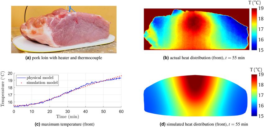
www.nature.com/scientificreports/
within the object. Landmann et al.10 reported a method that combined 2D IR data and depth data in the form of
a high-speed acquisition tool constructed of the light sensor and long-wave IR camera. The system returns a 3D
model with temperature data on its surface. A similar approach, merging thermal and depth data, was described
by Chromy and Z alud11. The proposed RoScan consisted of an IR camera, a color camera, and a laser scanner.
Schollemann et al.12 involved a similar idea, yet 3D computed tomography volume constituted the depth data.
Chen et al.13 proposed a 3D IR imaging approach for power systems evaluation using a series of 2D IR images
acquired around the enclosed heat source. The technique employed the intersection method to reconstruct
volumetric temperature data of an object.
A significant advantage of the third group of studies can be found in employing only the data generated
by IR cameras. This paper falls into this category, in which only individual studies have been reported so far.
Koutsantonis et al.16 presented a tomographic image reconstruction method in IR tomography, called RISE
(Reconstructed Image from Simulations Ensemble), combining statistical physics concepts and Monte Carlo
methods. The goal was to extract the physical parameters of an object and simulate a pack of image configura-
tions corresponding to a tomographic problem solution. The process was evaluated using a simulated dataset and
experimental data obtained from a thermal phantom. The method showed increased quality than two reference
reconstruction methods: algebraic reconstruction technique (ART)18 and maximum-likelihood expectation-
maximization (MLEM)19. However, the phantom medium employed in this study differs from the human body
tissue in terms of absorbance. Sage et al.17 reported preliminary results on 3D thermal reconstruction from a
series of 2D IR images for medical purposes. The reconstruction involved a backprojection method over an aga-
rose phantom. The initial effects indicated the ability to distinguish areas of abnormal temperature distribution
that correspond to the actual location of the heat source.
This study is a development of our research from Sage et al.17. For thermal tomography purposes, we employed
deep learning. The capability of deep learning applied to different kinds of medical image processing and analysis
has been a major issue in the last decade in terms of, e.g., image classification, object detection, semantic seg-
mentation, or registration20. A review by Ben Yedder et al.21 lists several methods designed for medical image
reconstruction using deep neural networks, yet none of them addresses IR imaging. The convolutional neural
networks (CNN) application scope broadens rapidly, also in terms of the input image shape and size. The original
works and models were designed for 2D images. Yet, with the consistent development of both hardware resources
and implementation concepts also the analysis of 3D structures became applicable in a reasonable time. CNNs
have increased attention in the field of medical image processing as the models constitute a fusion of deep learn-
ing and image processing methods22. The presence of convolutional layers enables the extraction of features from
the image. The spatial relations are crucial for complete image understanding, and the CNN preserves them.
Additionally, pooling layers guarantee the elimination of irrelevant features, hence the number of trainable
parameters and computation power requirements decrease. CNNs support the control of possible overfitting
and secure invariance to local translation22–24. For all those reasons, CNN appears as a suitable approach for
infrared image p rocessing25. Several studies reported the employment of recurrent neural networks (RNN) for
image operations, including segmentation and classification26–28. However, their main application fields are text
and audio processing. In contrast to CNN, the RNN primarily operates on sequential (time-domain) data. It is
also considered sensitive to the exploding or vanishing gradient problems, and the extraction of image features is
more robust in C NNs26,28. Here, we design and train a deep model (CNN) analyzing an input volume containing
initial tomographic reconstruction from planar thermal images.
This paper concisely presents the novel concept of CNN-based thermal tomography and the experimental
setup in both synthetic and real data with single or multiple heat sources. The original contribution brought by
the study can be found in: (1) the employment of deep learning into the field of thermal tomography, (2) inves-
tigating the ability to reconstruct the heat distribution from planar thermal images, and (3) supporting synthetic
design and validation of the model with the experimental setup involving a real object (pork) heated from a single
source. We also assess reconstruction performance using benchmark metrics. Our results prove the capability of
a deep model to reflect the temperature distribution inside the object and set the starting point for further devel-
opment of the method. We expect the knowledge-based model designed and trained for thermal tomography to
make an essential contribution to artificial intelligence-based computer-aided diagnosis and decision-making.
The materials and methods are described in “Materials and methods” section, including generation and
validation of the synthetic data and specification of our deep model for thermal reconstruction. “Results” sec-
tion presents a series of experiments over both synthetic and real data. The results and perspectives for artificial
intelligence-based thermal tomography are discussed in “Discussion” section. “Conclusion” section concludes
the study.
Materials and methods
Synthetic dataset. The synthetic dataset was prepared using a computer simulation using MATLAB Par-
tial Differential Equation Toolbox with the general formula:
dT
ρCp − ∇ · (k∇T) = f , (1)
dt
where T is the temperature, k—the thermal conductivity, ρ—the mass density, Cp denotes the specific heat, and f
is the heat generated inside the object ( f = 0 in our case). We created a 3D cylindrical phantom with a diameter
of 10 cm and a height of 5 cm using B lender29 software (V2.93 Blender Foundation, https://www.blender.org/)
and exported it to the .stl file (Fig. 1a). The heat source was a 0.5 cm diameter sphere with a variable location
inside the phantom. The distance d of the heat source center from the phantom axis toward the side wall varied
Scientific Reports | (2022) 12:2347 | https://doi.org/10.1038/s41598-022-06076-z 2
Vol:.(1234567890)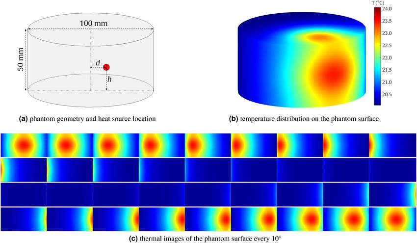
www.nature.com/scientificreports/
Figure 1. Illustration of the synthetic dataset generation from a cylindrical phantom.
Parameter Symbol Value Unit
Thermal conductivity k 0.49 W/(m ◦C)
Mass density ̺ 1103 kg/m 3
Specific heat Cp 3322 J/(kg ◦C)
Table 1. Thermal properties of muscle tissue used in phantom heat transfer simulation.
from 0.5 to 4.5 cm with a step of 0.5 cm. The same range was used to change the height h at which the heat source
was placed. This allowed for 81 unique combinations of object locations within the phantom.
Prepared models of the phantom and source geometry were used in heat transfer a nalysis30. For the phantom
interior, we set the thermal properties comparable to muscle tissue31. The exact values are given in Table 1. Instead
of providing the heat source explicitly, we used the Dirichlet boundary condition with a constant temperature
of 50◦ C on the source surface during the transient analysis. In each case, the initial temperature of the phantom
was 20◦ C. The same value of ambient temperature and the radiation emissivity coefficient of 0.95 served as the
boundary conditions for the phantom surface. Minkina and Dudzik32 have shown that two main quantities can
significantly influence temperature measurement errors: object emissivity and ambient temperature, while other
parameters under consideration: relative humidity, camera-to-object distance, and atmospheric temperature, do
not contribute to the error. We treated the initial temperature as a reference and modeled the heat distribution
in a differential manner ( T in relation to 20◦C). For high thermal contrast, the source temperature during the
simulation was 50◦ C ( T = 30◦C). We prepared several states of the model that resemble the heat distribu-
tion. The states were captured in 5-minute intervals from the 15th to the 60th minute from the beginning of the
simulation (Fig. 1b, c). Hence, the synthetic database contained a total of 810 unique thermal models.
For the mesh independence study, we verified a sequence of maximum mesh edge lengths from 5 cm down to
4 mm (descending order). The assumed model geometry produced meshes consisting of ca. 500 to 75,000 nodes.
To assess the mesh, we measured the maximum temperature Tmax in the object surface nodes in the 60th minute.
Figure 2 presents the results of two experiments with various heat source locations (d = 0.5 and 2.5 cm; h = 2.5
cm in both cases). Since the 0.1% change is considered a reliable indicator of the mesh i ndependence33,34, we set
the maximum mesh edge length to 0.5 cm in our study, obtaining ca. 40,000 nodes. That gave us sufficient reso-
lution to produce projections of acceptable quality, comparable to the actual measurements with an IR camera.
Denser mesh significantly increased the time consumption with a negligible impact on the quality of the model.
We also validated the simulation for conformity with the theoretical heat transfer. We used the general heat
conduction equation (1) for transient problems in a 3D space to calculate the analytical solution. Like in our
Scientific Reports | (2022) 12:2347 | https://doi.org/10.1038/s41598-022-06076-z 3
Vol.:(0123456789)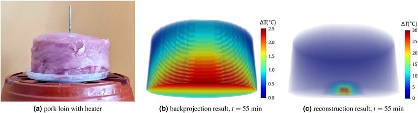
www.nature.com/scientificreports/
Figure 2. Maximum temperature of the model surface Tmax vs. the number of nodes in the mesh independence
study. (a) shows the absolute relative changes of Tmax from (b) in subsequent mesh sizes. The dashed line shows
the 0.1% level in (a).
Figure 3. Validation of the model: illustration of the setup in the cylindrical coordinate system (a) and
temperature distribution on the cylinder radius originating in the heat source center (red profile in (b),
z = h = 2.5 cm) (b).
simulation, we assumed a homogeneous and isotropic object with a constant thermal conductivity k. Considering
our phantom geometry, we used the heat conduction equation in a 3D cylindrical coordinate system35:
∂ 2T 1 ∂T 1 ∂ 2T ∂ 2T f 1 dT
2
+ + 2 2
+ 2 + = , (2)
∂r r ∂r r ∂φ ∂z k α dt
where r, z, φ are cylindrical coordinates (Fig. 3a), and α = ρCk p is the thermal diffusivity. For simplicity, we placed
our spherical heat source in the middle of the cylinder (d = 0, h = 2.5 cm), so the temperature distribution does
not depend on the φ angle. Moreover, f = 0, as we model the heat source surface by the Dirichlet boundary
condition. Therefore, Eq. (2) takes the form:
∂ 2T 1 ∂T ∂ 2T 1 dT
2
+ + 2 = , (3)
∂r r ∂r ∂z α dt
The outer boundary condition on the cylinder surface is defined in the radiation terms:
∂T
= εσ T 4 − T∞
4
(4)
−k − ,
∂→n
where ε denotes the radiation emissivity coefficient, σ —the Stefan–Boltzmann constant, − →
n is a vector normal to
the surface, and T∞ is the ambient temperature. We solved Eq. (3) using a forward-time central-space (FTCS)
scheme36 with appropriate space and time resolution to secure stability. Then, we compared the result with the
corresponding simulation obtained from the finite element method using Matlab PDE T oolbox37,38. Figure 3b
presents the temperature distribution on the cylinder radius on the heat source height (z = h = 2.5 cm, red pro-
file in Fig. 3a). The results are compliant, and the temperature differences decrease when nearing the surface. We
also measured the maximum temperature on the cylinder surface after 1 hour of heating, obtaining the 0.07◦ C
difference between the simulation and theoretical calculations.
Scientific Reports | (2022) 12:2347 | https://doi.org/10.1038/s41598-022-06076-z 4
Vol:.(1234567890)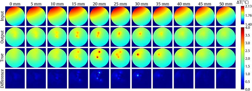
www.nature.com/scientificreports/
Figure 4. General scheme of the CNN model for thermal model reconstruction.
Planar thermal images and initial tomographic reconstruction. The initial reconstruction process
employed a series of 2D thermal images composed of synthetically generated data (Fig. 1c). The camera rotat-
ing around the object allows for observing temperature distribution on the surface at various angles (360 views
with a 1 ◦ resolution). To obtain individual reconstructions of 2D sections, we employed the backprojection
algorithm39. In the backprojection reconstruction, each pixel placed at the orientation of a given projection takes
a measured projection value. The process repeats for the entire set of angles, and values of corresponding pixels
are summed. Finally, the result is divided by the total number of projections. A stack of properly arranged 2D
slices finally constructs a 3D volume.
Due to the specifics of infrared radiation, 3D thermal volumes generated using the considered method require
further processing to achieve final reconstruction. Areas of increased temperature are located close to the edges
of the phantom, so volumetric temperature data is not reliable. Hence, the next stage employs deep learning to
improve the accuracy of heat distribution reconstruction within a given medium.
Convolutional neural network for thermal model reconstruction. To reconstruct the temperature
distribution, we designed a deep convolutional network of an autoencoder architecture (Fig. 4). The input layer
accepts a 100×100×50 volume, padded with zeros to fit the 128×128×50 size. The encoder path consists of four
processing blocks. Each involves a 2D convolutional layer (32, 64, 128, 256 filters, 3×3 kernel) followed by batch
normalization, leaky rectified linear unit (ReLU), and max pooling (2×2 stride). The decoder path involves four
segments, each performing transposed convolutions (256, 128, 64, and 32 filters, respectively, 3×3 kernel, 2×2
stride), batch normalization, and leaky ReLU activation. The reconstruction produces a 100×100×50 volume of
thermal tomography data.
The network was trained using the adaptive moment estimation (Adam) optimizer. We randomly partitioned
the database of 810 original volumes into the training, validation, and test subsets with an 80%:10%:10% ratio.
To extend the database and increase generalization capabilities, we applied data augmentation in each training
epoch by rotating every 3D volume by ten random angles in the axial plane. Hence, a single training sample
yielded ten rotated images per epoch. The batch size was set to 32, and the maximum number of epochs to 500.
We set both parameters experimentally to gain the highest efficiency and maintain low computational time.
Evaluation metrics. To assess our framework, we employed several well established metrics. Three were
taken from Koutsantonis et al.16: normalized mean square error (NMSE), correlation coefficient (CC), being a
spatial similarity measure between two images, and peak signal-to-noise ratio (PSNR). From Wang et al.40, we
adopted the structural similarity index (SSIM).
Finally, we propose a measure for heat source location error (HSLE). It is defined as a distance in millimeters
between the reference and the reconstructed heat source midpoint.
Scientific Reports | (2022) 12:2347 | https://doi.org/10.1038/s41598-022-06076-z 5
Vol.:(0123456789)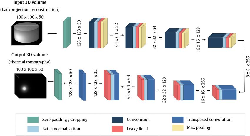
www.nature.com/scientificreports/
Metrics Mean ± std. dev. Median (25–75 percentile)
NMSE 0.036 ± 0.049 0.021 (0.013–0.035)
CC 0.981 ± 0.026 0.989 (0.981–0.993)
PSNR 43.135 ± 3.386 43.239 (40.856–45.556)
SSIM 0.748 ± 0.114 0.790 (0.697–0.826)
HSLE 1.398 ± 1.146 0.967 (0.689–1.592)
Table 2. Summary of testing the method over a synthetic dataset.
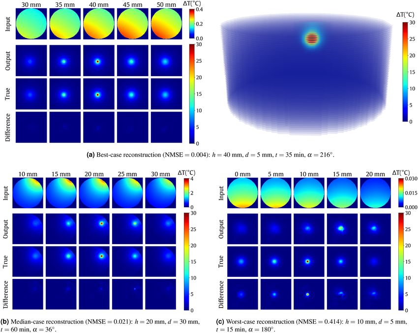
Figure 5. Visualization of the reconstruction results. Top to bottom in each subplot with projections:
backprojection slices, final tomographic reconstruction slices, ground-truth slices, the difference between the
reconstruction and ground truth (reconstruction error). In each case, the central column contains the heat
source center. The location (height) of each slice is given above the column. Volumetric visualization of the
reconstruction outcome is given in (a) (see Supplementary Video S1).
Results
Tests over a synthetic dataset. The original test set coming from a partition described in “Materials
and methods” section consisted of 81 unique cases. To extend the testing experiment, we rotated each volume
nine times around the main axis with a 36◦ increment (the α angle). This yielded a set of 810 unique test cases.
Full testing results are given in Table 2. Figure 5 presents selected visualizations, including the worst-case and
best-case reconstructions in terms of NMSE. For best-case recostruction visualization see also Supplementary
Video S1.
We also estimated the reconstruction time. Most of the time was consumed by the backprojection (113 s per
case). The thermal reconstruction using a trained deep model took 0.015 s per case. The tests were performed on
Scientific Reports | (2022) 12:2347 | https://doi.org/10.1038/s41598-022-06076-z 6
Vol:.(1234567890)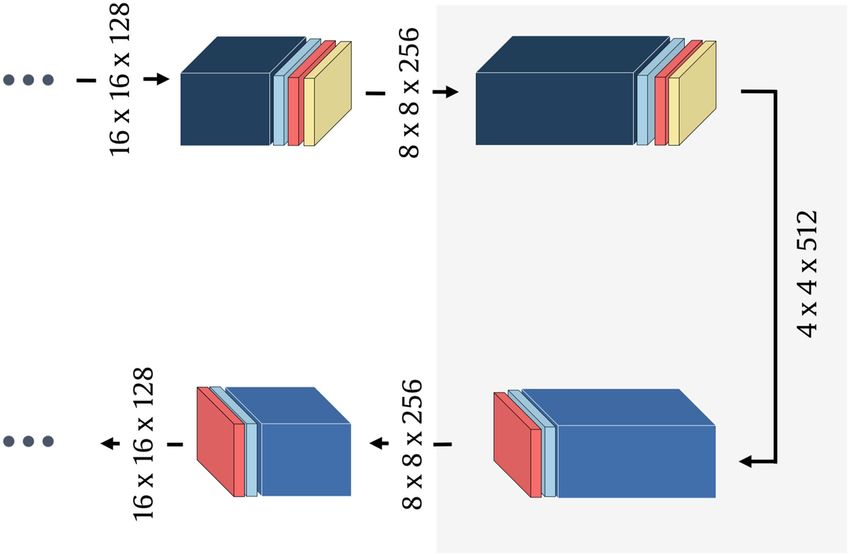
www.nature.com/scientificreports/

                                  Figure 6.  Model evaluation (experiment #1) using a pork loin (a), the obtained heat map (b), and heat map
                                  from the numerical model (d) on the front of the loin. The chart (c) shows the actual an simulated maximum
                                  temperature (front of the loin).

                                  Figure 7.  Model evaluation (experiment #2): the cylindrical pork object (a), backprojection (b) and
                                  reconstruction results (c).

                                  a workstation running a 64-bit Windows 10 operating system with an Intel Core i7-8750H CPU, 16 GB DDR4
                                  RAM, and GeForce GTX 1060 GPU with 1280 CUDA cores and 6 GB GDDR5 RAM.

                                  Experimental validation of the model. We numerically evaluated the assumptions for our model in two
                                  experiments involving pork meat of approximately known thermal properties (Table 1). The meat used in the
                                  experiments was in no way related to the animal experiments and did not require the approval of the bioethics
                                  committee.
                                      In the first experiment, we used a ca. 0.6 kg pork loin with a resistive heater placed inside (Fig. 6a) at about 3
                                  cm distance from the front (flat side). The measurement stand was surrounded by foam to limit the influence of
                                  the surroundings. The heater (a cement 39 , 10 W resistor with external package dimensions of 10 × 12 × 32
                                  mm) was supplied using a regulated power source. A thermocouple-based digital thermometer controlled its
                                  temperature to be 50◦ C. During heating, we acquired multiple static thermal images of the front of the loin.
                                  Figure 6b presents the thermal map obtained at the front after 55 min of the experiment. The corresponding heat
                                  map from our numerical model is shown in Fig. 6d. Figure 6c compares the simulated (red) and actual (blue)
                                  maximum temperature on the front of the loin.
                                      The second experiment involved pork cut in a cylinder with a ca. 10 cm diameter and 5 cm height (Fig. 7a).
                                  The meat was placed on a rotary table with markings every 10◦ . The same resistive heater was controlled by an
                                  Arduino-based temperature controller, battery-powered, and placed under the model to enable a free rotation of
                                  the stand. The heater temperature was first stabilized at 50◦ C and then inserted from the bottom into the meat
                                  cylinder about d = 15 mm from the central axis. Then, after 15, 25, 35, 45, and 55 minwe rotated the table and
                                  captured a full set of 2D thermal images every 10◦ . Figure 7b and c present the example reconstruction in the

Scientific Reports |   (2022) 12:2347 |                https://doi.org/10.1038/s41598-022-06076-z                                                     7

                                                                                                                                                 Vol.:(0123456789)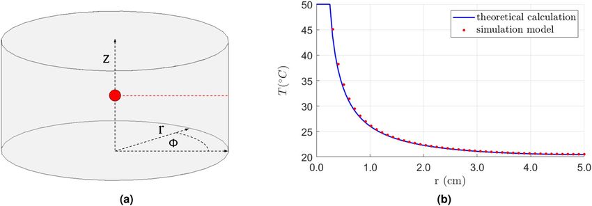
www.nature.com/scientificreports/
Metrics Mean ± std. dev. Median (25–75 percentile)
NMSE 0.019 ± 0.010 0.016 (0.012–0.023)
CC 0.978 ± 0.011 0.981 (0.971–0.987)
PSNR 37.354 ± 1.633 37.562 (36.408–38.521)
SSIM 0.952 ± 0.016 0.957 (0.948–0.963)
HSLE 3.597 ± 2.053 3.196 (2.064–4.722)
Table 3. Summary of testing the method over a synthetic dataset with a single low-temperature heat source.
Original model (four-block CNN) Extended model (five-block CNN)
Metrics Mean ± std. dev. Median (25–75 percentile) Mean ± std. dev. Median (25–75 percentile)
NMSE 0.022 ± 0.017 0.016 (0.012–0.025) 0.014 ± 0.017 0.008 (0.007–0.012)
CC 0.971 ± 0.020 0.977 (0.968–0.981) 0.980 ± 0.021 0.987 (0.982–0.989)
PSNR 29.579 ± 2.005 29.314 (28.545–30.649) 32.082 ± 2.852 31.834 (30.487–33.661)
SSIM 0.841 ± 0.074 0.849 (0.786–0.900) 0.904 ± 0.040 0.910 (0.879–0.938)
Table 4. Summary of testing the method over a synthetic dataset with multiple low-temperature heat sources.
55th minute through backprojection and by our trained model, respectively. In the simulation, the maximum
temperature T = 48.31◦C ( T = 30.31◦C) was detected d = 5 mm from the axis, at h = 5 mm.
Experiments with low‑temperature heat sources. After verifying our original assumptions over a
synthetic dataset and a real object, we prepared additional experiments to check the method’s capability to
handle lower temperature differences. The experiments refer to the original setup described in “Materials and
methods” section and “Tests over a synthetic dataset” section in terms of both materials and methods. All modi-
fications are depicted in the following sections.
Single heat source. First, we took synthetic phantoms with all 81 unique locations of the heat source (“Synthetic
dataset” section) and set five different temperatures to produce T = 1, 2, 3, 4, 5◦C (405 cases). Those relative
temperatures can be considered low compared to the original value of T = 30◦C. During training, we again
additionally rotated the phantoms with a 36◦ increment to produce 4050 unique cases. This time, we generated
a single thermal state per case in terms of heating time. Moreover, since the temperature difference was low, the
heat distribution was prepared after 300 min of heating. The validation results are shown in Table 3 using the
same metrics as before.
Multiple heat sources. Finally, we extended the low-teperature heat distribution investigation by involving mul-
tiple heat sources per phantom. For that purpose, we produced 1000 phantoms with random arrangements of
1–5 heat sources, each of a random 1–5◦ C temperature. In each case, the minimum distance between the centers
of any two sources was 10 mm (5 mm between their surfaces). Again, we captured a single heat distribution per
phantom after 300 min. The validation results of our deep model are presented in the left part of Table 4. We did
not determine the HSLE in this case, as it is a metrics designed for single-source setups.
We also verified the multi-source setup using the extended deep model. One processing block was added
to both encoder and decoder in the rightmost part form Fig. 4. The five-block encoder produces the 4×4×512
volume (Fig. 8). The results in the right part of Table 4 show the improvement brought by deepening the network.
Figure 9 presents the visualization of the best-case reconstructions in terms of NMSE (see also Supplementary
Video S2).
Discussion
The employment of deep learning to 3D tomographic reconstruction from planar thermal images has been the
central concept of our study. The results we present support this idea. We started our research in17 with the use
of backprojection reconstruction over a heated phantom and 2D IR images of a relatively low resolution (36
images with a 10◦ step). Since the IR radiation is not as penetrating as the ionizing one used in, e.g., computed
tomography or SPECT, the backprojection has a limited utility. That brought the idea of training a deep model
over a series of synthetic data of known properties and heat distributions. Evaluation of the trained model over
a synthetic dataset produced at least satisfactory results with low error measures and high spatial similarity
between the ground truth and the reconstructed heat distributions.
In all previous studies on thermal tomography, the shape of an object was simplified to a cylindrical form13,15,16.
We used the same approach here, but the proposed method itself does not have to be limited to one shape. We
can prepare synthetic data from any model with specific thermal properties for the training process. Compared
to Koutsantonis et al.16, our original idea involves a single heat source with a sphere geometry. Contrary to
RISE16, our results take into account distinct thermal contrast resulting from simulation with varying heating
Scientific Reports | (2022) 12:2347 | https://doi.org/10.1038/s41598-022-06076-z 8
Vol:.(1234567890)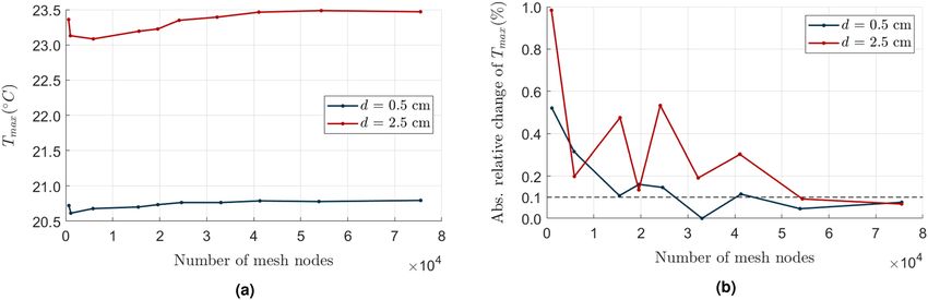
www.nature.com/scientificreports/
Figure 8. Illustration of the extension of the CNN model from Fig. 4. Added blocks are highlighted with a gray
background.
Figure 9. Visualization of the best-case reconstruction (NMSE = 0.004) in the multiple-heat-source
experiment with a five-block CNN. Top to bottom: backprojection slices, final tomographic reconstruction
slices, ground-truth slices, the difference between the reconstruction and ground truth (reconstruction error).
The location (height) of each slice is given above the column. For volumetric visualization of the reconstruction
outcome, see Supplementary Video S2.
times. Moreover, Koutsantonis’s study addressed semi-transparent medium; we do not set such constraints. Our
method allows for a better representation of the temperature distribution in the vicinity of the source compared
to the most simplified cases in16 (two identical heat sources). We obtained a higher SSIM index, reflecting the
visual similarity of the reconstruction and the original image. Our reconstruction is less noisy with higher PSNR
values: 43.135 on average than the best-case 33.25 in RISE. Both approaches reliably map the source temperature
and location with comparable NMSE and CC levels. We also prove the location mapping correctness using the
proposed HSLE metrics with the median below 1 mm.
Scientific Reports | (2022) 12:2347 | https://doi.org/10.1038/s41598-022-06076-z 9
Vol.:(0123456789)www.nature.com/scientificreports/
The most significant errors appeared when the source was d = 0.5 cm from the central axis of the object, h = 1
cm from the bottom, after 15 min of heating. Two other cases from the test set with d = 0.5 cm and after 15 min
were reconstructed well (with h = 2.5 and 3 cm), so the error does not come from the proximity of the source
to the central axis. We find the other reasons in a short time to spread the heat towards the external surface and
specific temperature distribution at the object edge.
Our thermographic reconstruction simulation was verified in some aspects based on the actual measurements
of the physical model. We are fully aware of the limitations of this double experiment (“Experimental validation
of the model” section): the location (depth) and dimensions of the object and the heat source (inside the resistor),
which are difficult to reproduce in a simplified model accurately, tissue inhomogeneity, or non-insulated base.
We are also aware of the limitations of the model: the simplified geometry, homogeneous internal structure, no
base. Figures 6b and d show that tissue heterogeneity and shape imperfections contribute to the reconstruction
inaccuracy. Moreover, we found some errors in the heat source height estimation. These may result from the
influence of the bed on the heat dissipation process, not considered in the simulations. Additional disturbing
factors were the ca. 3 min time needed to perform the complete IR acquisition cycle or possible extra heat from
the electronic circuitry supplying the heater (under the object). However, taking into account the obtained results
and their compliance with the model (Figs. 6c, 7c), despite all the limitations and simplifications, we believe that
the method is promising for the appropriate reconstruction of real-object volumetric temperature distribution.
In this pilot study on CNN-based reconstruction, we mainly focused on simulating a single heat source of a
basic shape (a spherical heat source). Except for the physical model experiment, we did not investigate models
different from cylindrical. The natural further development direction is to investigate more complex forms and
shapes through model training and validation. We believe that the deep model can follow such structures, per-
haps through some superposition of learned patterns. Diversification of the training and test sets by introducing
rotations of the original data supported this assumption: the network performed equally well regardless of the
rotation angle. In “Experiments with low-temperature heat sources” section, we aimed at verifying more complex
tasks in terms of heater temperature and the number of heat sources. Lowering the relative source temperature
T from 30 to 5 ◦ C and less did not result in a decreased performance. Hence, the model can produce robust
reconstruction regardless of T with the applied assumptions. We also made another step forward by randomly
placing up to five low-temperature heat sources in a single phantom. The obtained results are promising (Table 4,
Fig. 8). The network trained with multi-source phantoms reconstructs the temperature distribution affected by
the mutual influence of several sources. The exact temperature of particular sources themselves remains an issue.
However, in single-source testing cases, both the heater temperature and location are estimated correctly, so the
properties of the two previous models are retained. Extending the model with additional convolution blocks
increased its capacity, thanks to which it was possible to obtain better results while increasing the complexity of
the data set. The reconstructions are visually smoother, which is also reflected in improved PSNR values.
So far, our framework involves the backprojection algorithm as an intermediate step between IR image
acquisition and thermal reconstruction. However, we consider avoiding it in our future research, also due to
significant time consumption. That would enable reconstructing the heat distribution based directly on a series
of planar IR images of the object. However, such an approach will require studies on the optimal arrangement
of IR images in the deep model input in terms of spatial relationships.
Conclusion
Our study introduces the artificial intelligence concept into a relatively poorly explored field of thermal tomogra-
phy. Our results show the capability of a deep model to reconstruct the volumetric temperature distribution from
a sequence of planar thermal images of an object containing variable number of heat sources. We find the idea
promising and share it with the scientific community with some plans for developing the method and models.
Received: 26 August 2021; Accepted: 24 January 2022
References
1. Lahiri, B., Bagavathiappan, S., Jayakumar, T. & Philip, J. Medical applications of infrared thermography: A review. Infrared Phys.
Technol. 55, 221–235. https://doi.org/10.1016/j.infrared.2012.03.007 (2012).
2. Roslidar, R. et al. A review on recent progress in thermal imaging and deep learning approaches for breast cancer detection. IEEE
Access 8, 116176–116194. https://doi.org/10.1109/ACCESS.2020.3004056 (2020).
3. Hristov, J. Bio-heat models revisited: Concepts, derivations, nondimensalization and fractionalization approaches. Front. Phys. 7,
189. https://doi.org/10.3389/fphy.2019.00189 (2019).
4. Kabiri, A. & Talaee, M. R. Analysis of hyperbolic Pennes bioheat equation in perfused homogeneous biological tissue subject to
the instantaneous moving heat source. SN Appl. Sci. 3, 1–8. https://doi.org/10.1007/s42452-021-04379-w (2021).
5. Pennes, H. H. Analysis of tissue and arterial blood temperatures in the resting human forearm. J. Appl. Physiol. 85, 5–34. https://
doi.org/10.1152/jappl.1998.85.1.5 (1998).
6. Levy, A., Dayan, A., Ben-David, M. & Gannot, I. A new thermography-based approach to early detection of cancer utilizing
magnetic nanoparticles theory simulation and in vitro validation. Nanomed. Nanotechnol. Biol. Med. 6, 786–796, https://doi.org/
10.1016/j.nano.2010.06.007 (2010).
7. Sadeghi, M. et al. Feasibility test of dynamic cooling for detection of small tumors in IR thermographic breast imaging. Curr.
Direct. Biomed. Eng. 5, 397–399. https://doi.org/10.1515/cdbme-2019-0100 (2019).
8. Lim, S. & Yoon, Y. J. Phase compensation technique for effective heat focusing in microwave hyperthermia systems. Appl. Sci..
https://doi.org/10.3390/app11135972 (2021).
9. Kim, D., Hernandez, D. & Kim, K.-N. Design of a dual-purpose patch antenna for magnetic resonance imaging and induced RF
heating for small animal hyperthermia. Appl. Sci.https://doi.org/10.3390/app11167290 (2021).
Scientific Reports | (2022) 12:2347 | https://doi.org/10.1038/s41598-022-06076-z 10
Vol:.(1234567890)www.nature.com/scientificreports/
10. Landmann, M. et al. High-speed 3D thermography. Opt. Lasers Eng. 121, 448–455. https://doi.org/10.1016/j.optlaseng.2019.05.
009 (2019).
11. Chromy, A. & Zalud, L. The roscan thermal 3d body scanning system: Medical applicability and benefits for unobtrusive sensing
and objective diagnosis. Sensors. https://doi.org/10.3390/s20226656 (2020).
12. Schollemann, F. et al. An anatomical thermal 3D model in preclinical research: Combining CT and thermal images. Sensors. https://
doi.org/10.3390/s21041200 (2021).
13. Chen, C.-Y., Yeh, C.-H., Chang, B. & Pan, J.-M. 3D reconstruction from IR thermal images and reprojective evaluations. Math.
Probl. Eng. 1–8, 2015. https://doi.org/10.1155/2015/520534 (2015).
14. Krȩcichwost, M. et al. Chronic wounds multimodal image database. Comput. Med. Imaging Graph.https://doi.o rg/1 0.1 016/j.c ompm
edimag.2020.101844 (2021).
15. Toivanen, J. et al. Thermal tomography utilizing truncated Fourier series approximation of the heat diffusion equation. Int. J. Heat
Mass Transf. 108, 860–867. https://doi.org/10.1016/j.ijheatmasstransfer.2016.12.060 (2017).
16. Koutsantonis, L., Rapsomanikis, A.-N., Stiliaris, E. & Papanicolas, C. N. Examining an image reconstruction method in infrared
emission tomography. Infrared Phys. Technol. 98, 266–277. https://doi.org/10.1016/j.infrared.2019.03.015 (2019).
17. Sage, A., Ledwoń, D., Juszczyk, J. & Badura, P. 3D thermal volume reconstruction from 2D infrared images—a preliminary study.
In booktitleInnovations in Biomedical Engineering, vol. 1223 of seriesAdvances in Intelligent Systems and Computing, 371–379.
(Springer, Cham, 2021). https://doi.org/10.1007/978-3-030-52180-6_38.
18. Gordon, R., Bender, R. & Herman, G. T. Algebraic reconstruction techniques (ART) for three-dimensional electron microscopy
and X-ray photography. J. Theor. Biol. 29, 471–481. https://doi.org/10.1016/0022-5193(70)90109-8 (1970).
19. Shepp, L. A. & Vardi, Y. Maximum likelihood reconstruction for emission tomography. IEEE Trans. Med. Imaging 1, 113–122.
https://doi.org/10.1109/TMI.1982.4307558 (1982).
20. Litjens, G. et al. A survey on deep learning in medical image analysis. Med. Image Anal. 42, 60–88. https://d oi.o rg/1 0.1 016/j.m edia.
2017.07.005 (2017).
21. Ben Yedder, H., Cardoen, B. & Hamarneh, G. Deep learning for biomedical image reconstruction: A survey. Artif. Intell. Rev. 54,
215–251. https://doi.org/10.1007/s10462-020-09861-2 (2021).
22. Liu, X., Song, L., Liu, S. & Zhang, Y. A review of deep-learning-based medical image segmentation methods. Sustainability. https://
doi.org/10.3390/su13031224 (2021).
23. Sarvamangala, D. & Kulkarni, R. Convolutional neural networks in medical image understanding: A survey. Evol. Intell. 1–22.
https://doi.org/10.1007/s12065-020-00540-3 (2021).
24. Singh, S. P. et al. 3D deep learning on medical images: A review. Sensors. https://doi.org/10.3390/s20185097 (2020).
25. He, Y. et al. Infrared machine vision and infrared thermography with deep learning: A review. Infrared Phys. Technol. 116, 103754.
https://doi.org/10.1016/j.infrared.2021.103754 (2021).
26. Alzubaidi, L. et al. Review of deep learning: Concepts, CNN architectures, challenges, applications, future directions. J. Big Data.
https://doi.org/10.1186/s40537-021-00444-8 (2021).
27. Chakravarty, A. & Sivaswamy, J. Race-net: A recurrent neural network for biomedical image segmentation. IEEE J. Biomed. Health
Inform. 23, 1151–1162. https://doi.org/10.1109/JBHI.2018.2852635 (2019).
28. Hesamian, M. H., Jia, W., He, X. & Kennedy, P. Deep learning techniques for medical image segmentation: Achievements and
challenges. J. Digit. Imaging 32, 582–596. https://doi.org/10.1007/s10278-019-00227-x (2019).
29. organizationBlender Foundation, addressStichting Blender Foundation, Amsterdam. Blender - a 3D modelling and rendering
package (2018).
30. The MathWorks, Inc. Partial Differential Equation Toolbox. addressNatick, MA, United States (2021).
31. Mcintosh, R. L. & Anderson, V. A comprehensive tissue properties database provided for the thermal assessment of a human at
rest. Biophys. Rev. Lett. 5, 129–151. https://doi.org/10.1142/S1793048010001184 (2010).
32. Minkina, W. & Dudzik, S. Infrared thermography: Errors and uncertainties (Wiley, 2009).
33. Subramaniam, V., Dbouk, T. & Harion, J.-L. Topology optimization of conductive heat transfer devices: An experimental investiga-
tion. Appl. Therm. Eng. 131, 390–411. https://doi.org/10.1016/j.applthermaleng.2017.12.026 (2018).
34. Turgay, M. B. & Yazıcıoğlu, A. G. Numerical simulation of fluid flow and heat transfer in a trapezoidal microchannel with comsol
multiphysics: A case study. Numer. Heat Transf. Part A Appl. 73, 332–346. https://doi.org/10.1080/10407782.2017.1420302 (2018).
35. Han, J.-C. Analytical Heat Transfer (Taylor & Francis, 2012).
36. Balaji, C., Srinivasan, B. & Gedupudi, S. Heat Transfer Engineering: Fundamentals and Techniques (Academic Press, 2020).
37. Ali, N. et al. Numerical simulation of time-dependent non-Newtonian nanopharmacodynamic transport phenomena in a tapered
overlapping stenosed artery. Nanosci. Technol. Int. J. 9, 247–282. https://doi.org/10.1615/NanoSciTechnolIntJ.2018027297 (2018).
38. Beg, O. A., Zaman, A., Ali, N., Gaffar, S. A. & Beg, E. T. Numerical computation of nonlinear oscillatory two-immiscible magne-
tohydrodynamic flow in dual porous media system: FTCS and FEM study. Heat Transfer-Asian Res. 48, 1245–1263. https://doi.
org/10.1002/htj.21429 (2019).
39. Bruyant, P. Analytic and iterative reconstruction algorithms in spect. J. Nucl. Med. Off. Publ. Soc. Nucl. Med. 43, 1343–58 (2002).
40. Wang, Z., Bovik, A. C., Sheikh, H. R. & Simoncelli, E. P. Image quality assessment: From error visibility to structural similarity.
IEEE Trans. Image Process. 13, 600–612. https://doi.org/10.1109/TIP.2003.819861 (2004).
Acknowledgements
This research was supported by the Polish Ministry of Science and Silesian University of Technology statutory
financial support No. 07/010/BK_22/1011 (BK-231/RIB1/2022).
Author contributions
All authors are justifiably credited with authorship. The detailed contribution is as follows: D.L. - conceptual-
ization, methodology, software, validation, formal analysis, investigation, data curation, original draft writing,
manuscript review & editing, visualization; A.S. - conceptualization, methodology, software, resources, data
curation, original draft writing; J.J. - conceptualization, investigation, funding acquisition, project administration;
M.R. - investigation, resources, original draft writing, manuscript review & editing; P.B. - original draft writing,
manuscript review & editing, supervision.
Competing interests
The authors declare no competing interests.
Additional information
Supplementary Information The online version contains supplementary material available at https://doi.org/
10.1038/s41598-022-06076-z.
Scientific Reports | (2022) 12:2347 | https://doi.org/10.1038/s41598-022-06076-z 11
Vol.:(0123456789)www.nature.com/scientificreports/
Correspondence and requests for materials should be addressed to D.L.
Reprints and permissions information is available at www.nature.com/reprints.
Publisher’s note Springer Nature remains neutral with regard to jurisdictional claims in published maps and
institutional affiliations.
Open Access This article is licensed under a Creative Commons Attribution 4.0 International
License, which permits use, sharing, adaptation, distribution and reproduction in any medium or
format, as long as you give appropriate credit to the original author(s) and the source, provide a link to the
Creative Commons licence, and indicate if changes were made. The images or other third party material in this
article are included in the article’s Creative Commons licence, unless indicated otherwise in a credit line to the
material. If material is not included in the article’s Creative Commons licence and your intended use is not
permitted by statutory regulation or exceeds the permitted use, you will need to obtain permission directly from
the copyright holder. To view a copy of this licence, visit http://creativecommons.org/licenses/by/4.0/.
© The Author(s) 2022
Scientific Reports | (2022) 12:2347 | https://doi.org/10.1038/s41598-022-06076-z 12
Vol:.(1234567890)You can also read