Tracing Versus Freehand for Evaluating Computer-Generated Drawings
←
→
Page content transcription
If your browser does not render page correctly, please read the page content below
Tracing Versus Freehand for Evaluating Computer-Generated Drawings
ZEYU WANG, Yale University
SHERRY QIU, Yale University
NICOLE FENG, Carnegie Mellon University
HOLLY RUSHMEIER, Yale University
LEONARD MCMILLAN, University of North Carolina at Chapel Hill and Mental Canvas, Inc.
JULIE DORSEY, Yale University and Mental Canvas, Inc.

Fig. 1. Progression of drawings. (a) One of 100 image prompts in our dataset. (b) Apparent ridges rendered from the geometry. (c) Progression of density map
of tracings binned into temporal quintiles. (d) Progression of density map of registered freehand drawings binned into temporal quintiles. All drawings of the
prompt are superimposed. Note the spatio-temporal similarities between tracing and freehand drawing. Contours are drawn early and tone details later. Fossil
model by Digital Atlas of Ancient Life on Sketchfab (CC0 1.0).

Non-photorealistic rendering (NPR) and image processing algorithms are                        is no quantitative evaluation of tracing as a proxy for freehand drawing. In
widely assumed as a proxy for drawing. However, this assumption is not                        this paper, we compare tracing, freehand drawing, and computer-generated
well assessed due to the difficulty in collecting and registering freehand                    drawing approximation (CGDA) to understand their similarities and differ-
drawings. Alternatively, tracings are easier to collect and register, but there               ences. We collected a dataset of 1,498 tracings and freehand drawings by
                                                                                              110 participants for 100 image prompts. Our drawings are registered to the
Authors’ addresses: Zeyu Wang, Yale University, 51 Prospect St, New Haven, CT, 06511,         prompts and include vector-based timestamped strokes collected via stylus
zeyu.wang@yale.edu; Sherry Qiu, Yale University, 51 Prospect St, New Haven, CT,
06511, sherry.qiu@yale.edu; Nicole Feng, Carnegie Mellon University, 500 Forbes Ave,          input. Comparing tracing and freehand drawing, we found a high degree
Pittsburgh, PA, 15213, nfeng@andrew.cmu.edu; Holly Rushmeier, Yale University, 51             of similarity in stroke placement and types of strokes used over time. We
Prospect St, New Haven, CT, 06511, holly.rushmeier@yale.edu; Leonard McMillan,                show that tracing can serve as a viable proxy for freehand drawing because
University of North Carolina at Chapel Hill and Mental Canvas, Inc. 201 S Columbia            of similar correlations between spatio-temporal stroke features and labeled
St, Chapel Hill, NC, 27599, mcmillan@cs.unc.edu; Julie Dorsey, Yale University and
Mental Canvas, Inc. 51 Prospect St, New Haven, CT, 06511, julie.dorsey@yale.edu.              stroke types. Comparing hand-drawn content and current CGDA output, we
                                                                                              found that 60% of drawn pixels corresponded to computer-generated pixels
Permission to make digital or hard copies of all or part of this work for personal or         on average. The overlap tended to be commonly drawn content, but people’s
classroom use is granted without fee provided that copies are not made or distributed         artistic choices and temporal tendencies remained largely uncaptured. We
for profit or commercial advantage and that copies bear this notice and the full citation
on the first page. Copyrights for components of this work owned by others than ACM
                                                                                              present an initial analysis to inform new CGDA algorithms and drawing
must be honored. Abstracting with credit is permitted. To copy otherwise, or republish,       applications, and provide the dataset for use by the community.
to post on servers or to redistribute to lists, requires prior specific permission and/or a
fee. Request permissions from permissions@acm.org.
© 2021 Association for Computing Machinery.
                                                                                              CCS Concepts: • Applied computing → Arts and humanities; • Human-
0730-0301/2021/8-ART52 $15.00                                                                 centered computing → User studies; • Computing methodologies →
https://doi.org/10.1145/3450626.3459819                                                       Non-photorealistic rendering; Perception.

                                                                                                     ACM Trans. Graph., Vol. 40, No. 4, Article 52. Publication date: August 2021.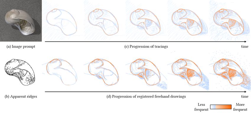
52:2 • Zeyu Wang, Sherry Qiu, Nicole Feng, Holly Rushmeier, Leonard McMillan, and Julie Dorsey

Additional Key Words and Phrases: sketch dataset, drawing process, stroke             • A comparison between tracing and freehand drawing through
analysis                                                                                a spatio-temporal analysis, in which we demonstrate their
                                                                                        similarities in stroke placement and drawing progression.
ACM Reference Format:                                                                 • A comparison of CGDA results with hand-drawn data, in
Zeyu Wang, Sherry Qiu, Nicole Feng, Holly Rushmeier, Leonard McMillan,                  which we show that current CGDA methods capture about
and Julie Dorsey. 2021. Tracing Versus Freehand for Evaluating Computer-
                                                                                        60% of pixels drawn and suggest areas for improvement.
Generated Drawings. ACM Trans. Graph. 40, 4, Article 52 (August 2021),
12 pages. https://doi.org/10.1145/3450626.3459819
                                                                                2 RELATED WORK
                                                                                2.1 A Taxonomy of Hand-Drawn Datasets
1    INTRODUCTION                                                               There has been enormous work on datasets and algorithms for vari-
The computer graphics and image processing communities have                     ous drawing applications. As shown in Table 1, large-scale datasets
long been interested in developing methods that resemble free-                  like TU-Berlin [Eitz et al. 2012], Sketchy [Sangkloy et al. 2016],
hand drawing. These computer-generated drawing approximations                   and QuickDraw [Ha and Eck 2018] are intended for sketch recogni-
(CGDA) are often used as a proxy for hand drawings. For example,                tion and image retrieval. The use of text prompts in these datasets
several recent deep learning-based applications [Isola et al. 2017;             leaves room for participants’ interpretations and encourages sym-
Li et al. 2018; Su et al. 2018] have relied exclusively on CGDA for             bolic sketches. While valuable for machine learning applications,
training data. However, the extent to which current CGDA results                many of these sketches do not reflect the complexity of observa-
actually resemble real drawings remains unclear. In particular, most            tional drawing. In addition to freehand sketches, tracings, which
CGDA methods only approximate the end result of drawing, ne-                    are directly registered to the prompt, have been collected to study
glecting the drawing process which includes stroke and temporal                 image segmentation and contour extraction. Tracing datasets like
information. In this paper, we compare current CGDA methods with                BSDS500 [Arbeláez et al. 2011] and PhotoSketch [Li et al. 2019] illus-
both freehand drawing and tracing, in order to better model the                 trate people’s perception of edges and contours, which is essential
process and content of drawing and inform new algorithms.                       to creating a good drawing [Suwa and Tversky 1997].
   Tracing is a form of hand drawing commonly used in art and                      More related to our motivation are the drawing datasets used
design that has not been compared with freehand drawing or CGDA                 to understand how artists and designers draw, including Prince-
output. Tracings are easier to obtain than freehand drawings and are            ton [Cole et al. 2008], Portrait [Berger et al. 2013], OpenSketch [Grya-
registered to image prompts by definition. Like freehand drawing,               ditskaya et al. 2019], and GMU [Yan et al. 2020]. The Portrait and
tracing can also provide temporal information and stroke demarca-               OpenSketch datasets include temporal information to analyze the
tion. Comparisons of tracing to freehand drawing have been long                 process of portrait drawing and technical drafting. The OpenSketch
discussed in the art community [Jamieson 2019], but there is a lack             and GMU datasets include contours and additional types of strokes
of quantitative analysis. Therefore, we consider tracing as a proxy             that reveal people’s drawing intention. Because it is hard to col-
for freehand drawing and also compare it to CGDA, thus enabling                 lect high-quality data, these datasets are relatively small in scope
new paradigms for data collection and algorithm evaluation.                     (portrait photos or diffuse renderings) and size (one or two dozen
   This study compares tracing, freehand drawing, and CGDA out-                 prompts and usually at most ten artists per prompt). Therefore, it
put based on a collection of tracings and freehand drawings. Our                remains necessary to create a dataset of timestamped representa-
data have vector and temporal information and are registered to                 tional drawings with a wider variety of prompts, artists, and stroke
image prompts. We observed that in both freehand drawing and                    types in order to further understand how people trace and draw.
tracing, the types of strokes drawn over time are similar; common
contours are drawn early and tone details occur later in the drawing            2.2    Computer-Generated Drawing Approximation
process (Fig. 1). We found that in both forms of drawing, similar
                                                                                The computer graphics community has been interested in creating
correlations exist between stroke features and time as well as be-
                                                                                NPR techniques to render various artistic styles. Different algo-
tween stroke features and drawing intention. This suggests that
                                                                                rithms for generating lines have been proposed in order to imitate
tracing can serve as a viable proxy for freehand drawing and jus-
                                                                                human-drawn strokes. Suggestive contours [DeCarlo et al. 2003] ex-
tifies this efficient method of drawing data collection. In addition,
                                                                                tend true contours of shapes; ridges and valleys [Ohtake et al. 2004]
we evaluated current CGDA methods by comparing their output to
                                                                                and apparent ridges [Judd et al. 2007] depict salient surface features;
both freehand drawing and tracing and found a 60% overlap. This
                                                                                neural contours incorporate multiple line extractors [Liu et al. 2020];
reveals aspects of CGDA methods that require more attention, such
                                                                                and hatching strokes [Kalogerakis et al. 2012; Praun et al. 2001] con-
as the drawing process and different types of strokes. We expect
                                                                                vey material, tone, and form. These NPR techniques take a 3D model
our dataset and analysis to be useful for many applications, includ-
                                                                                as input, examine differential properties such as surface curvatures,
ing data-driven CGDA, stroke type classification, drawing process
                                                                                and produce lines in the form of static bitmaps. In the image domain,
simulation, sketch-based modeling, and sketch beautification.
                                                                                edge detection can generate lines at the boundary of high-contrast
   This paper makes the following contributions:
                                                                                regions. Various image processing techniques produce edge maps to
     • A dataset of 1,498 tracings and freehand drawings of 100                 imitate drawing, such as the extended difference-of-Gaussians [Win-
       image prompts by 110 participants, with temporal, vector,                nemöller et al. 2012], holistically-nested edge detection [Xie and Tu
       and pressure information that are registered to the prompts.             2015], and contour extraction from images [Li et al. 2019].

ACM Trans. Graph., Vol. 40, No. 4, Article 52. Publication date: August 2021.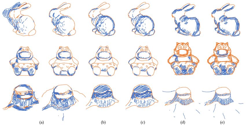
Tracing Versus Freehand for Evaluating Computer-Generated Drawings •                          52:3

Table 1. A taxonomy of drawing datasets. Our dataset includes both tracings and registered freehand drawings composed of vector-based timestamped
strokes. The wide variety of prompts, participants, and stroke types presented in our dataset allows us to study general tendencies in drawing.

                                              Temporal                    Shading &                          People                            Freehand
                  Dataset                                  Registration                   Prompts                            Tracings
                                                data                       texture                          /prompt                            drawings
     TU-Berlin [Eitz et al. 2012]                ✓              ✗             ✗              250              ∼80                 0               20k
    Sketchy [Sangkloy et al. 2016]               ✓              ✗             ✗              125              ∼600                0               75k
    QuickDraw [Ha and Eck 2018]                  ✓              ✗             ✗              345             ∼145k                0              50m
    BSDS500 [Arbeláez et al. 2011]               ✗              ✓             ✗              500              4–9               2,696              0
     PhotoSketch [Li et al. 2019]                ✓              ✓             ✗             1,000              5                5,000              0
     Princeton [Cole et al. 2008]                ✗              ✓             ✗               12              1–11               208              208
     Portrait [Berger et al. 2013]               ✓              ✓             ✓               24               7                  0               672
 OpenSketch [Gryaditskaya et al. 2019]           ✓              ✓             ✓               12              7–15                0               417
        GMU [Yan et al. 2020]                    ✗              ✓             ✓              141              3–5                526              281
         SpeedTracer (ours)                      ✓              ✓             ✓              100             11–21              1,210             288

   Recently, CGDA techniques have become widely used to generate           the study of general consistency and variation between tracing and
training data for sketching applications based on deep learning. For       freehand drawing. Our detailed analysis provides insight into the
example, many use convolutional neural networks (CNN) to learn             drawing process and informs future drawing applications.
the inverse mapping from NPR to shape, such as reconstructing
normal maps [Su et al. 2018] and dense 3D point clouds [Lun et al.
2017], predicting parameters for procedural modeling [Huang et al.         3 DATA COLLECTION
2017], and creating caricature face models [Han et al. 2017] and           3.1 Study Design
other freeform surfaces [Delanoy et al. 2018; Li et al. 2018] from
drawings. While CGDA is commonly used as a proxy for drawing,              3.1.1 Prompt selection. Past studies have used text prompts to col-
this assumption lacks evaluation. In particular, although some CGDA        lect sketches for recognition and image retrieval. Text prompts are
techniques simulate the process of observational drawing [Liu et al.       less specific and encourage varying interpretations. As a result,
2014], most of them neglect the order in which people draw and             sketches are often symbolic or caricatured. To encourage more real-
artists’ drawing intention. Our work aims to understand the process        ism and to support registration, we used visual prompts in a similar
of tracing and freehand drawing, which could inform new methods            manner to the analysis of portrait drawing [Berger et al. 2013]. The
that better emulate drawing.                                               image prompt was visible throughout a drawing session, so that the
                                                                           artist could observe and make various drawing decisions.
                                                                              We included a total of 100 photorealistic images from various
2.3   Tracing vs. Freehand Drawing
                                                                           sources, with wide variations in appearance (unicolor diffuse vs. tex-
Tracing is a common tool and practice in art and design. Art stu-          tured and specular) and content (single objects vs. complex scenes).
dents learn to observe proportions by looking at an object through         We chose diverse shapes with abundant geometric and visual fea-
a glass viewfinder with grids and drawing over it [Edwards 2012].          tures rather than simple uniform shapes. Specifically, there were
Architects also trace and selectively reuse lines for communicat-          33 rendered images from publicly available 3D models with appear-
ing and iterating design ideas [Johannessen and Van Leeuwen                ance assets, 21 images from photometric stereo datasets [Shi et al.
2017]. Drawing interfaces such as ShadowDraw [Lee et al. 2011],            2016; Toler-Franklin et al. 2007; Xiong et al. 2015; Zhang 2012] with
DrawAFriend [Limpaecher et al. 2013], ShadowModel [Fan et al.              associated normal maps, 30 images used for raster pencil drawing
2013], and EZ-Sketching [Su et al. 2014] leverage a tracing metaphor       production [Lu et al. 2012], 9 images of 3D-printed objects from
to help users create more realistically proportioned drawings and          multiple viewpoints [Slavcheva et al. 2018], and 7 photographs of
models. Although tracing is easier to produce than freehand draw-          sculptures. The image content ranged from clay animals to furniture
ing, the art community has long discussed the distinction between          pieces to landscapes. Overall, this collection covers a wide range of
these two forms. While tracing helps artists understand structure          shapes and scenes with diverse reflectance properties.
and perspective, it can also discourage detailed analysis of the work
and become a crutch [Jamieson 2019]. Quantitative comparisons
between tracing and freehand drawing mainly take place in psy-             3.1.2 Constraints. Many previous studies instructed participants to
chology, focusing on eye-hand interactions, brain activities, and          draw only contour strokes. However, drawings typically employ a
drawing skills using simple shapes [Gowen and Miall 2006, 2007;            wider range of strokes including those that represent tone, shadows,
Ostrofsky et al. 2012]. However, they are not readily applicable to        textures, and those accentuating important details. In order to cap-
observational drawing and computer graphics.                               ture these different types of strokes, we did not limit the types that
   This paper aims to advance understanding of how people trace            participants could draw. On the other hand, we found time limits
and draw by collecting timestamped drawings and including a wider          used in previous studies helpful for encouraging participants to
variety of prompts, participants, and stroke types. Our dataset allows     prioritize strokes and for collecting normalized data. We imposed a

                                                                                  ACM Trans. Graph., Vol. 40, No. 4, Article 52. Publication date: August 2021.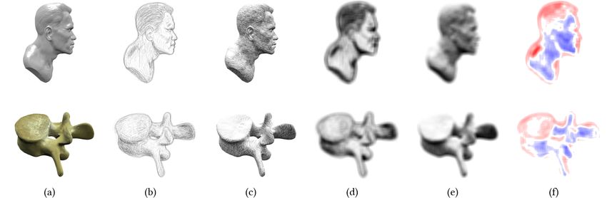
52:4 • Zeyu Wang, Sherry Qiu, Nicole Feng, Holly Rushmeier, Leonard McMillan, and Julie Dorsey

time limit of two minutes based on observations from a pilot study—
most people could complete the overall content within two minutes
and still had time to add details such as shading and texture.

3.2    Implementation
3.2.1 Drawing interface. We implemented SpeedTracer, a web-based
drawing interface using Vue.js [You 2020]. Our drawing interface is
composed of a square canvas with an image prompt and an optional
blank canvas with user options on the sides of the webpage. We
use square canvases with images scaled and padded to 800×800 as
this is close to the prompts’ original resolutions. Participants were
instructed to trace over the image or draw on the blank canvas using
a digital stylus. The interface provides the ability to select stroke
width, color, and opacity, undo or redo a stroke, and clear the canvas.
Stroke width is determined by multiplying user-specified width and
pen pressure, allowing varying widths and tapering. Participants
could change stroke color for artistic purposes and better tracing
visibility. Strokes were stored in vector format in a database with             Fig. 2. Registration of freehand drawings using a composite of collected
timestamps, pressure, and appearance properties. Each participant               tracings as a guide. (a) Image prompt. (b) Composite of tracings. (c) Sample
traced or drew a prompt only once but could trace or draw multiple              freehand drawings. (d) Same freehand drawings after registration.
prompts. The prompts were ordered such that each prompt would
be completed by a similar number of participants.
                                                                                3.3    Drawing Registration
3.2.2 Participants. A total of 110 participants contributed to our
                                                                                In order to compare freehand drawings to tracings and CGDA re-
dataset. Among them, 85 were professional illustrators, experienced
                                                                                sults, we need to first register them to the image prompt. We use
students from art and architecture schools, students enrolled in a
                                                                                tracings to aid in registration by maximizing the correlation be-
college drawing class, or amateur drawing enthusiasts. To enrich the
                                                                                tween each freehand drawing and a composite of all tracings of the
dataset with easier-to-collect crowdsourced data used in machine
                                                                                same prompt over a displacement field. We implemented a coarse-to-
learning research, the remaining 25 participants were recruited
                                                                                fine optimization framework using ImageRegistrationMethod()
from Amazon Mechanical Turk for the tracing task. 39 participants
                                                                                in the Insight Segmentation and Registration Toolkit (ITK) [Kitware
contributed tracings using a 28-inch Microsoft Surface Studio with
                                                                                2020]. The first step was to initialize a reasonable displacement field
the Surface Pen in our lab. Others used their own tablets with stylus
                                                                                at full resolution. Our automatic initialization used a global affine
support such as an iPad with the Apple Pencil and Wacom tablets.
                                                                                transformation, followed by B-spline transformations at three scales
All freehand drawings were collected remotely.
                                                                                from an image pyramid. Freehand drawings that included many
   In all, there were 46 males, 62 females, and two who identified as
                                                                                background strokes occasionally led to a bad initialization. To ad-
non-binary gender. Their ages ranged from 18 to 61 years, with an
                                                                                dress these cases, we manually labeled 18 to 42 fiducials in both the
average age of 27. Of these, 59 had two or more years of art training,
                                                                                freehand drawing and the image prompt, and initialized the displace-
20 had one year, and 31 had none. Participants reported an average
                                                                                ment field by fitting a thin plate spline model. The second step was to
of four years of art training with the most experienced reporting
                                                                                maximize the correlation between the freehand drawing and the trac-
38 years. Each participant contributed 1–50 tracings or freehand
                                                                                ing composite using gradient descent to obtain the optimal displace-
drawings, with an average of 14. 13 participants were left-handed.
                                                                                ment field. We used the following parameters: 256×256 resolution,
Most participants were volunteers and not compensated. We paid
                                                                                SetMetricAsANTSNeighborhoodCorrelation(radius=16), and
each of the 25 turkers $0.50 for 10 tracings, and each of the seven
                                                                                SetOptimizerAsGradientDescent(learningRate=1, numberOf-
artists recruited from mihuashi.com $7.68 for 15 freehand drawings.
                                                                                Iterations=300, estimateLearningRate=EachIteration).
3.2.3 Dataset. We excluded 187 tracings mostly by turkers because               Overall, the registered drawings share contours at nearby pixel loca-
they included only an outline or content unrelated to the prompt. We            tions (Fig. 2), which allows us to perform a spatio-temporal analysis
also excluded all 15 freehand drawings by one participant who had               on tracings and freehand drawings simultaneously.
no art training and drew only partial outlines. The resulting dataset
contains a total of 1,210 tracings from 96 participants and 288 free-           4     DRAWING ANALYSIS
hand drawings from 19 participants. Five artists contributed both               To compare tracing and freehand drawing, we examine similarity in
tracings and freehand drawings. We collected fewer freehand draw-               content drawn, stroke usage, and progression of drawing over time.
ings because they required more skill. We did not collect freehand              We then evaluate CGDA methods by finding the overlap between
drawings for 30 prompts of complex scenes because they would be                 their output and both tracing and freehand drawing. Our analysis
hard to register. Each of the remaining 70 prompts of single objects            includes 70 prompts of single objects with 851 tracings and 288
has about 12 tracings and 4 freehand drawings.                                  freehand drawings.

ACM Trans. Graph., Vol. 40, No. 4, Article 52. Publication date: August 2021.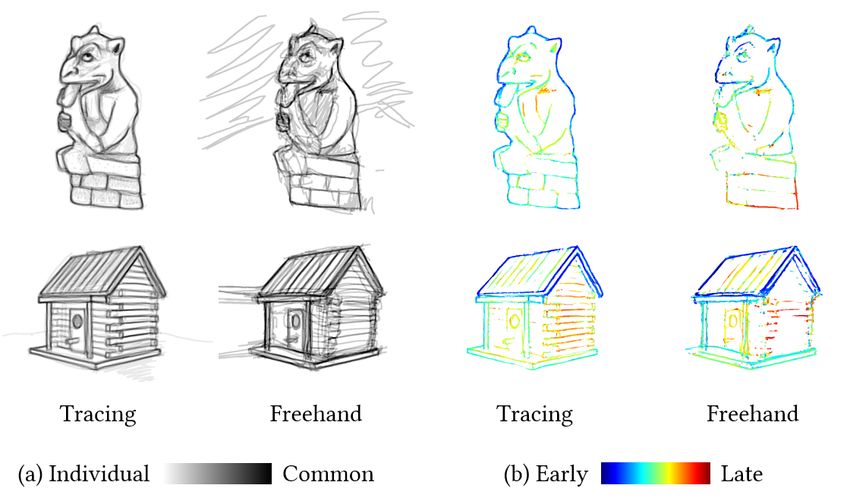
Tracing Versus Freehand for Evaluating Computer-Generated Drawings •                                                         52:5

4.1   Do People Draw Similar Content?
Our analysis begins with an exploration of the content and the way
people trace and draw. We rasterized collected tracings and regis-
tered freehand drawings to enable pixelwise comparisons across
drawings. We also leveraged temporal information to understand
the order pixels are covered during the drawing process.

4.1.1 What people draw in common. Inspired by previous analy-
sis [Cole et al. 2008], we explore common content within tracings,
within freehand drawings, and between tracings and freehand draw-
ings. We computed a histogram of pairwise distances between draw-
ings for both tracing and registered freehand drawing (Fig. 3c). For
every pixel in each drawing rasterized using one pixel-wide strokes,                        20%                                                      10%                           Tracing

                                                                          Pair percentage

                                                                                                                                  Pixel percentage
we recorded its closest chessboard distance in pixels to every other                        15%                                                       8%                           Freehand
drawing of the same prompt. For both forms of drawing across all                            10%                                                       6%
prompts, over 50% of the distances are close to a pixel in another                                                                                    4%
                                                                                            5%
                                                                                                                                                      2%
drawing (within four pixels) and about 15% of the distances are far                         0%                                                        0%

                                                                                                    0
                                                                                                    2
                                                                                                    4
                                                                                                    6
                                                                                                    8

                                                                                                  ≥20
                                                                                                   10
                                                                                                   12
                                                                                                   14
                                                                                                   16
                                                                                                   18
from any other drawing (more than 20 pixels).                                                                                                              1 3 5 7 9 11 13 15 17 19 21 23 25
   To demonstrate similarities between tracing and freehand draw-                                      Distance in pixels                                       Temporal bin index
                                                                                                     (c) Distance in pixels                                   (d) Temporal bin index
ing, we first generated density maps and quantified their overlap
(Fig. 3a). We superimposed all tracings of the same image prompt
                                                                         Fig. 3. Similarities between tracing and freehand drawing. (a) Density maps
to create a density map for tracing, and similarly with all registered   of two sample prompts. (b) Commonly drawn regions (CDR) colored by the
freehand drawings of the same prompt. To compensate for imperfect        average time at which each pixel is drawn. (c) Histograms of pairwise closest
registration, we dilated the raster drawings for two iterations before   distances between pixels for all prompts. (d) Histograms of the number of
superimposition so two strokes four pixels apart can overlap. We         CDR pixels over time for all prompts. Note the decreasing trend.
thresholded the density map using half the number of participants
to obtain a binary commonly drawn region (CDR). We computed
a histogram of pairwise distances between CDR pixels in tracing
and freehand drawing, and found that over 80% of the distances are          Findings: In both tracing and freehand drawing, the number of
within four pixels.                                                      all pixels drawn is mostly uncorrelated with time. However, people
   Findings: In both tracing and freehand drawing, over half of the      tended to draw more common pixels early, and this tendency is
pixels are common content. People also draw similar common con-          stronger in tracing.
tent between tracing and freehand drawing, and we observed that          4.1.3 Where people draw over time. After exploring when the com-
this mostly occurs at silhouettes and interior contours of objects.      mon content is drawn, we examine changes in focus over time as
                                                                         it relates to spatial locality. For CDR pixels of each prompt, we
4.1.2 When people draw common pixels. Drawing analysis should            recorded their (x, y) coordinates relative to the top left corner and
encompass both the end result and the drawing process. After ex-         their distance to the barycenter of the drawing (distc). We then com-
ploring what people draw in common, we examine when they draw            puted the Pearson correlation coefficient with a p-value between
the common content. We used the interpolated timestamps for each         these properties and time (Fig. 4a). We found that among all prompts
pixel to analyze how many pixels people draw over time. For each         90% in tracing have a significantly negative correlation between
drawing, we equally divided the temporal span into 25 bins and           distc and time, and 84% in freehand drawing have a significantly
counted the number of all pixels drawn within each temporal bin.         positive correlation between y and time.
We also counted the number of CDR pixels based on their average             To understand this tendency at a finer level, we divided the tem-
timestamp for each prompt (Fig. 3d). We computed the Pearson             poral span of each drawing into ten equal bins and took snapshots of
correlation coefficient with a p-value between the number of pixels      the drawing in progress. We then computed the convex hull area of
and the temporal bin index to understand how it changes over time.       each snapshot relative to that of the final drawing (Fig. 4b). The dif-
All analyses in this paper use a significance level of p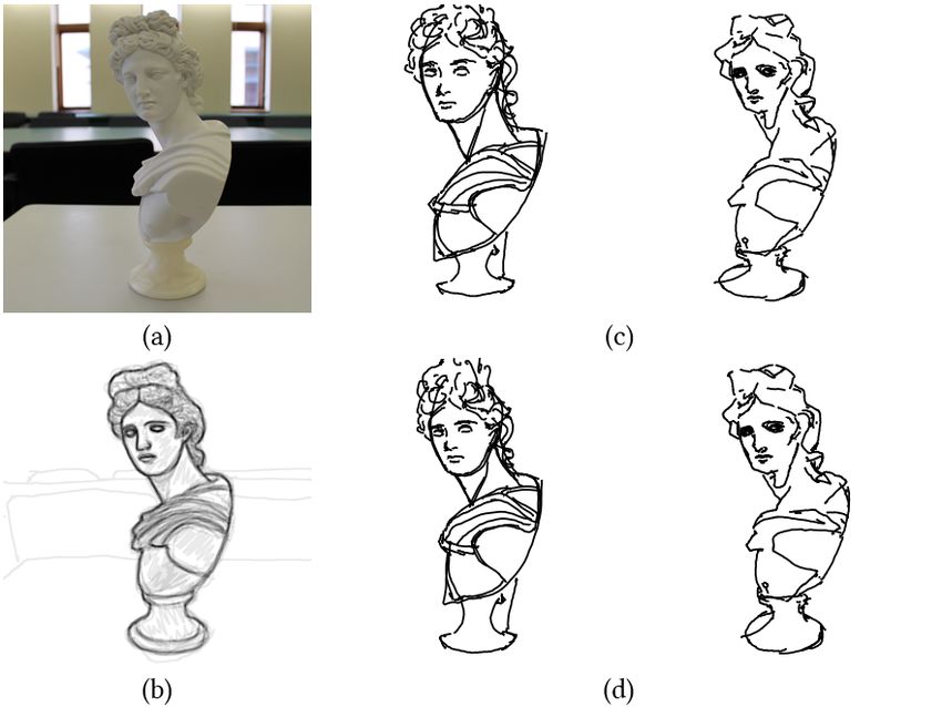
52:6 • Zeyu Wang, Sherry Qiu, Nicole Feng, Holly Rushmeier, Leonard McMillan, and Julie Dorsey
Percentage of drawings
x 57% 33% 10% 100% 15% Tracing 20%
y 59% 34% 7% 90% Freehand 15%
10%
80%
Convex hull area
distc 4% 90% 6% 10%
70% 5%
5%
Tracing
60% Tracing 0% 0%
x 66% 24% 10% 50% 0 100 200 0% 50% 100%
y 84% 14%2% 40% Freehand (a) Number of strokes (b) Pause in percentage of duration
distc 31% 66% 3% 30%
Percentage of drawings
20% 15%
Freehand drawing 20%
1 2 3 4 5 6 7 8 9 10 10%
(a) SigPos SigNeg Insig (b) Temporal bin index 10%
5%
Fig. 4. Stroke placement over time. (a) Percentage of prompts with correla- 0% 0%
0 20000 40000 0 20000 40000
tions between pixel location (x, y) in the CDR and time. distc: distance to the
(c) Number of pixels (d) Accumulated stroke lengths in pixels
barycenter of the drawing. SigPos: significant positive correlation, SigNeg:
significant negative correlation, Insig: insignificant correlation. (b) Convex 15%
Percentage of strokes
20%
hull area over time. In tracing, a larger area is covered earlier due to a
10%
stronger tendency to draw outside-to-inside than in freehand drawing. 10%
5%
0% 0%
0 250 500 0 1000 2000
ANOVA shows that the temporal difference of commonly drawn con-
tent between tracing and freehand drawing is significantly smaller (e) Stroke length in pixels () Stroke speed in pixels per second
if the prompt does not contain any facial features (p = 0.0099).
Fig. 5. Distributions across all drawings: (a) the number of strokes in each
4.2 Do People Use Similar Strokes? drawing, (b) total duration of pauses in each drawing, as percentage of time
While a raster representation shows the consistency across draw- used for entire drawing, (c) the number of pixels in each rasterized drawing,
(d) accumulated stroke lengths in each drawing, (e) the arc length of each
ings, information about individual strokes is lost. To understand
stroke, and (f) the speed of each stroke. The dashed vertical line represents
whether people use similar strokes in tracing and freehand draw- the median. The last point is an overflow bin except in (b).
ing, we analyze the distribution of vector stroke statistics, stroke
ordering, and how stroke features change over time.
4.2.1 Distribution of basic statistics. We computed four statistics energy function using heuristics such as simplicity, proximity, and
for each tracing and each registered freehand drawing: number of collinearity [Fu et al. 2011]. The energy function captures unary
strokes, pauses as percentage of total drawing duration, number and binary costs and is defined as
of pixels, and accumulated stroke lengths. We also computed two
statistics for each stroke: arc length and speed. Fig. 5 shows their n−1
Õ n−2
Õ
distributions in tracing and freehand drawing. In tracing, the number E =w c ind (li )θ (i) + c tra (li , li+1 ),
of strokes has a median of 61, pause duration 49%, number of pixels i=0 i=0
8382, accumulated stroke lengths 13105, stroke length 96, and stroke
where li is the i th stroke after ordering. c ind (l) = ηc str (l) + c cir (l)
speed 323. The corresponding statistics in freehand drawing are 78,
captures the complexity of an individual stroke, where c str (l) =
59%, 9246, 15769, 140, and 483. Since each prompt has a comparable
1 − straightness captures the deviation from a straight line and
number of collected drawings, these distributions can reflect general
c cir (l) = std(κ) captures the deviation from a constant-curvature
trends in tracing and freehand drawing.
circle. θ (i) = 1 − i/n is used to enforce the heuristic of simplicity,
Findings: We observed more flexible drawing behaviors in free-
i.e., simple strokes should be drawn first. c tra (li , l j ) = w pc pro (li , l j ) +
hand drawing than tracing. In freehand drawing, people tended to
(1 − w p )c col (li , l j ) captures the transition cost from stroke li to l j ,
draw more strokes and overdrawing is more common. People also
where the proximity term c pro (li , l j ) is the distance between the
tended to pause more possibly because they needed more time to
closest points on two strokes, and the collinearity term c col (li , l j ) is
consider the next part and its proportions when working with a
the positive angular difference between two endpoint tangents. We
blank canvas. Stroke length is more evenly distributed in freehand
used the exact definitions and weights w = 1, η = 0.1, w p = 1/9 by
drawing than in tracing. This agrees with our observation—when
Fu et al., and we refer the reader to their paper for more details.
tracing, people tended to draw long strokes at silhouettes followed
To understand if these heuristics play a similar role in tracing
by much shorter shading strokes, whereas people tended to use
and freehand drawing, we performed a Monte Carlo sampling of
many connecting strokes at silhouettes in freehand drawing.
all possible orderings of common strokes (defined in Section 4.4)
4.2.2 Comparing stroke ordering. To examine trends in the draw- in each drawing. For each ordering, we computed each term of the
ing process, we compare stroke ordering in tracing and freehand energy function using strokes before registration. A heuristic is
drawing by evaluating a list of heuristics used to assign order to considered important if the energy function takes a low value at
vector strokes. Specifically, finding a Hamiltonian path in a graph the ground-truth ordering compared to other random orderings. As
of strokes can generate a plausible drawing order by minimizing an shown in the inset table, we computed a score for each heuristic
ACM Trans. Graph., Vol. 40, No. 4, Article 52. Publication date: August 2021.Tracing Versus Freehand for Evaluating Computer-Generated Drawings • 52:7
and their combination as the percent of random orderings whose length 5% 47% 48% 16% 32% 52%
energy was above that of the ground-truth ordering.
Findings: Overall, these heuristics characterize stroke ordering dist 5% 47% 48% 9% 38% 53%
better in freehand drawing than tracing. Proximity is most im- duration 2% 59% 39% 13% 26% 61%
portant for both, suggesting that temporally neighboring strokes speed 50% 8% 42% 27% 17% 56%
tend to be spatially close. Collinearity comes second and is less
pressure 7% 56% 37% 39% 22% 39%
important in tracings, which Tracing Freehand
could be due to single long width 49% 38% 13% 78% 11%11%
c pro (li , l j ) 97.89% 99.81%
strokes in tracings versus opacity 13%
c col (li , l j ) 90.55% 97.62% 69% 18% 17% 74% 9%
shorter connecting strokes
E 81.35% 93.04%
in freehand drawings. Sim- (a) Tracing (b) Freehand drawing
c str (l) 44.16% 66.68%
plicity does not characterize SigPos SigNeg Insig
c cir (l) 31.42% 51.33%
stroke ordering effectively.
4.2.3 Stroke features over time. To further understand similarities Fig. 6. Percentage of drawings with a significantly positive, significantly
negative, or insignificant correlation between stroke features and time.
between strokes used in tracing and freehand drawing, we examine
how stroke features evolved throughout the drawing process. We
extracted features [Mahoney 2018] from each stroke before registra- 100% 100%
Percentage of strokes
tion and found their correlation to the time the stroke was completed.
80% 80%
Stroke features included arc length, distance between two endpoints
(dist), duration, speed, average pressure, stroke width, opacity, the 60% 60%
number of points, screen-space angle of the vector connecting the 40% 40%
two endpoints, average distance to image center, bounding box
coordinates, positions of two endpoints, curvature approximated 20% 20%
by nine uniformly sampled points on the stroke, and straightness 0% 0%
defined as dist/length. For every drawing, we computed the Pearson 0 1 0 1
correlation coefficient between each feature and time with a p-value. Normalized stroke order
We excluded drawings in which the correlation coefficient could not (a) Tracing (b) Freehand drawing
be computed, e.g., missing pressure or strokes of a fixed width. For
each feature, we computed the percentage of drawings with a signif- Silhouee Interior contour Ridge/valley
icantly positive, significantly negative, or insignificant correlation. Hatching Stipple Texture
We reported all correlation results to avoid data dredging.
As shown in Fig. 6, in both tracing and freehand drawing, opacity,
Fig. 7. Distribution of stroke types over time. Note the percentage of silhou-
duration, dist, and length tended to decrease over time, whereas
ettes at the beginning and hatching strokes towards the end.
width and speed tended to increase over time. An inconsistency was
pressure, as it mainly decreased over time only in tracing—people
tended to apply more pressure when they started tracing contours
for shading), stipple (dots for shading), and texture (color difference).
than drawing them on a blank canvas.
Fig. 7 shows the percentage of strokes for each type over time.
Findings: In both tracing and freehand drawing, early strokes such
Findings: Overall, we observed that drawings progressed similarly
as silhouettes tended to be long and drawn slowly using opaque
in tracing and freehand drawing. Silhouettes were dominant at the
colors. In contrast, late strokes such as hatching tended to be short
beginning and hatching strokes became more prominent towards
and drawn quickly using translucent colors and wider strokes.
the end. Interior contours and ridges and valleys appeared mainly in
the middle of the drawing process. Stipple and texture strokes were
4.3 How Do Drawings Develop Over Time? drawn infrequently. People drew more hatching in tracing than
Changes in stroke features over time indicate that people might in freehand drawing, possibly because freehand drawing required
employ multiple types of strokes with different drawing intention. more skill and people had less time to depict shading.
Therefore, it is important to understand if drawing intention evolves
similarly in tracing and freehand drawing. 4.3.2 Building stroke classifiers. Trends in how stroke features and
labels change over time suggest the possibility of stroke classifica-
4.3.1 Labeling drawing intention. The first author manually labeled tion. We built random forest classifiers to predict stroke type using
10,832 strokes in 130 tracings and 3,400 strokes in 42 freehand draw- features from Section 4.2 with 80% data for training and 20% for test-
ings for 10 prompts. All strokes fall into two main categories: geo- ing. We first performed robust standardization on the features using
metric contours and tone details. We further divided geometric the 5th and 95th percentiles of each feature. During training, we
contours into silhouettes (foreground-background separation), inte- used four-fold cross-validation to select optimal hyperparameters.
rior contours (depth discontinuity), and ridges and valleys (normal We split data in three different ways—splitting prompts, drawings,
discontinuity). We also divided tone details into hatching (strokes or strokes. Table 2 summarizes the ten-time average test accuracy
ACM Trans. Graph., Vol. 40, No. 4, Article 52. Publication date: August 2021.52:8 • Zeyu Wang, Sherry Qiu, Nicole Feng, Holly Rushmeier, Leonard McMillan, and Julie Dorsey
Fig. 8. Sample results of two stroke classifiers both predicting geometric contours (orange) and tone details (blue). The first classifier used 80% tracings as
training data and 20% tracings as test data. The second classifier used all tracings as training data and all freehand drawings as test data. (a) Labeled tracings
used in training for both classifiers. (b) Labeled test tracings for the first classifier. (c) Predicted labels by the first classifier. (d) Labeled test freehand drawings
for the second classifier. (e) Predicted labels by the second classifier, which shows models learned from tracings can be transferred to freehand drawings.
Table 2. Average test accuracy of random forest classifiers for predicting 4.4 How Much Do CGDA and Drawing Overlap?
stroke labels. The classifiers were trained using two labels and six labels,
and with different splits of data. After comparing tracing and freehand drawing, we revisit current
methods for computer-generated drawing approximation as they
Tracing Freehand drawing are commonly used as a proxy for hand drawings. CGDA methods
2 labels 6 labels 2 labels 6 labels fall into two classes: NPR methods that assume an underlying 3D
representation, and image processing methods that operate directly
Split prompts 75.57% 59.49% 84.24% 48.96%
on images. We compare both tracings and freehand drawings to
Split drawings 80.16% 66.67% 78.30% 53.52%
CGDA results to quantitatively establish whether their use is a
Split strokes 90.11% 82.99% 89.06% 69.40%
reasonable approximation to either form of drawing.
4.4.1 Precision and recall. Inspired by the analysis approach of
Cole et al. [2008], we start with a pixelwise comparison between
rasterized hand-drawn data and CGDA output. We computed preci-
sion and recall, where precision is the fraction of pixels in a CGDA
using two (contours, details) or six (silhouettes, interior contours, output that fall in a neighborhood of any pixel in the drawing. We
ridges and valleys, hatching, stipple, texture) labels. rasterized each stroke in the drawing and considered it to be cap-
The classifiers distinguished geometric contours from tone details tured by CGDA output if over half of its pixels fall in a neighborhood
with an accuracy of about 80% on splits of prompts and drawings, of any pixel in the CGDA image. We then measured recall as the
and an accuracy of about 90% on splits of strokes. The most im- fraction of pixels on such strokes captured by the CGDA output.
portant features for classification were time, length, duration, speed, We generated one-pixel wide CGDA output using five widely used
and straightness. Fig. 8 shows sample training data, ground truth for methods: suggestive contours (SC) [DeCarlo et al. 2003], ridges and
testing, and predictions using the classifier with 80% drawings as valleys (RV) [Ohtake et al. 2004], and apparent ridges (AR) [Judd
training data. In another experiment, we trained a classifier using et al. 2007] for 33 prompts rendered from 3D models as well as
all tracings and tested it on freehand drawings, which achieved an Canny edges [Canny 1986] and holistically-nested edges (HED) [Xie
average accuracy of 76.32% over all prompts. and Tu 2015] for all 70 prompts (Fig. 10). We chose thresholds for
Findings: A stroke’s temporal features can effectively characterize the algorithms such that the number of output pixels was closest
drawing intention in both tracing and freehand drawing. Further- to the median number of pixels in all tracings and freehand draw-
more, the high accuracy of classifying strokes in a freehand drawing ings of the same prompt. We used a 9×9 neighborhood based on
with a classifier trained on tracings suggests that models learned observations from the pairwise distances and a hybrid raster-vector
from tracings can be transferred to freehand drawings. representation to compensate for imperfect registration.
ACM Trans. Graph., Vol. 40, No. 4, Article 52. Publication date: August 2021.Tracing Versus Freehand for Evaluating Computer-Generated Drawings • 52:9
Precision (tracing) Precision (freehand) Recall (tracing) Recall (freehand)
100% 100% 100%
80% 80% 80%
60% 60% 60%
40% 40% 40%
20% 20% 20%
0% 0% 0%
SC RV AR Canny HED Geo Geo Img Img Geo Geo Img Img
(a) (b) (c)
Fig. 9. Precision and recall of NPR and image processing output compared with tracing and freehand drawing. (a) Average precision and recall for five types of
computer-generated output. (b) Average precision and recall on images with (gray) and without background. (c) Average precision and recall on images with
(gray) and without texture. Obj: object-space NPR output, i.e., SC+RV+AR. Img: image processing output, i.e., Canny+HED.
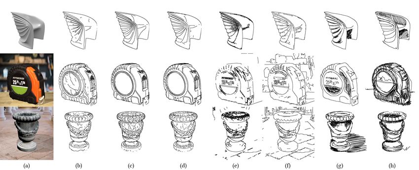
Fig. 10. Computer-generated results and drawings. (a) Image prompts. (b) Suggestive contours (SC). (c) Ridges and valleys (RV). (d) Apparent ridges (AR).
(e) Canny edges. (f) Thinned holistically-nested edges (HED). (g) Sample tracings. (h) Sample registered freehand drawings. A 3D model is required for (b)–(d).
Chair model by KarloBalboa on TurboSquid (royalty-free). Tape model by Artec Group, Inc. (CC BY 3.0). Vase model by 3dhdscan on Sketchfab (CC BY 4.0).
Findings: As shown in Fig. 9a, all CGDA methods used in our 45 contain texture. Using one way ANOVA, we found that for both
analysis achieved comparable precision and recall on tracing and tracing and freehand drawing, NPR output achieved lower precision
freehand drawing—about 60% of drawn content is consistent with and recall on image prompts containing background or texture. This
computer-generated output. A one-way ANOVA suggests that NPR agrees with our intuition because NPR typically does not consider
algorithms achieved higher precision than image processing al- image background or object texture. Image processing-based CGDA
gorithms although the difference in recall was not as significant. output achieved lower precision and recall on prompts with back-
SC and RV achieved comparable precision whereas AR achieved ground or texture for both forms of drawing, although the difference
higher precision. RV and AR achieved comparable recall whereas in recall is not as prominent. This can be explained by the fact that
SC achieved lower recall. Canny and HED achieved comparable image processing methods often include extraneous edges from
precision but Canny achieved higher recall than HED. AR is the background and texture areas that people do not necessarily draw.
best proxy for drawing among these methods. Findings: The disparity between precision and recall on different
prompts shows a gap between drawings and computer-generated
4.4.2 Image attributes. We observed that CGDA algorithms achieved results, and reveals that people employ diverse drawing strategies
different performance on different images. To better understand the when depicting complex prompts, e.g., non-diffuse and textured
disparity, we analyze how image attributes relate to the performance objects. Such prompts are lacking in previous drawing studies, and
of CGDA algorithms. We divided the image prompts based on their therefore the richness of hand-drawn data was not captured. This
attributes and computed the average precision and recall for CGDA analysis shows our dataset’s value for identifying extensions to NPR
results (Fig. 9bc). Among all 70 prompts, 39 have a background and and image processing algorithms that better approximate drawing.
ACM Trans. Graph., Vol. 40, No. 4, Article 52. Publication date: August 2021.52:10 • Zeyu Wang, Sherry Qiu, Nicole Feng, Holly Rushmeier, Leonard McMillan, and Julie Dorsey
4.4.3 Correlation with common strokes. In Section 4.1 (Fig. 3), we
discovered that people tended to depict a common set of contours,
and here we examine how these common strokes correspond to
computer-generated output. We used three density maps (tracing,
freehand drawing, CGDA) to compute two per-stroke metrics: com-
mon score and CGDA score. We rasterized each stroke, recorded
the maximum tracing or freehand drawing density in a 5×5 neigh- Tracing
borhood of each pixel along the stroke, and averaged the density
values over the entire stroke to compute the common score. Simi-
larly, we computed the CGDA score with a density map generated
by combining computer-generated results of all NPR and image
processing algorithms. Then, we computed the Pearson correlation
coefficients with a p-value between both scores and stroke order, as
well as between the two scores for all strokes in each drawing. Freehand drawing
As shown in Fig. 11d, the common score and the CGDA score (a) (b) (c)
tend to decrease over time. This decrease is more pronounced in
tracing. There is a significantly positive correlation between the common~order 3% 64%common~order
33% 5% 43% 52%
common score and the CGDA score in 85% or more of the tracings CGDA~order 5% 50% CGDA~order
45% 4% 36% 60%
and freehand drawings. On average, strokes captured by CGDA
CGDA~common CGDA~common
85% 15% 88% 12%
(score≥0.5) account for 62% pixels in tracing and 60% pixels in
freehand drawing, suggesting that about 40% of hand-drawn content Tracing Freehand drawing
remains uncaptured. (d) SigPos SigNeg Insig
Findings: CGDA methods can capture content that people com-
monly draw, but not the diverse artistic choices that people employ. Fig. 11. Correlation between stroke order, common score, and CGDA score.
4.4.4 Comparison with NPR hatching. We observed that in addi- (a) A drawing pseudocolored by stroke order. Warmer color represents later
tion to contours, people often depicted tone details using hatching. drawn strokes. (b) A drawing pseudocolored by common score. Warmer
color represents more commonly drawn strokes. (c) A drawing pseudocol-
Therefore, we compare drawing with NPR hatching [Praun et al.
ored by CGDA score. Warmer color represents strokes better captured by
2001] to determine how well NPR captures drawn shading. We first
CGDA. (d) Percentage of drawings with a significantly positive, significantly
created a composite of all drawings for each prompt and blurred negative, or insignificant correlation between common score, CGDA score,
the composite using a 25×25 box filter to get areas of dense stroke and stroke order. Note that common strokes tend to be captured by CGDA.
coverage. Then, we generated NPR hatching using the same config-
urations as the prompts and varied the light intensity so that the
hatching image blurred with the same box filter had a similar level of
overall response as the blurred drawing composite (Fig. 12). Similar
We computed the dot product between normal and view vectors
to the previous definition of precision and recall, we computed the
(N · V ) for 21 photometric stereo and 33 rendered prompts. We also
fraction of pixels in the blurred NPR hatching whose response was
computed nine object-space properties for the rendered prompts,
within 10% of total response range at the same pixel in the blurred
including the maximum, minimum, mean, and Gaussian curvatures,
drawing composite and vice versa.
the derivative of the maximum curvature in the corresponding direc-
In both tracing and freehand drawing, less than half of drawn
tion, the largest view-dependent principal curvature (ViewDepCurv)
shading is consistent with the hatching algorithm. For example,
and its derivative in the corresponding direction, the radial curva-
the algorithm generates uniform hatching in the hair and the face,
ture and its derivative in the radial direction. We used a random
whereas people place strokes primarily in the hair to demonstrate
forest regressor to construct a hierarchy of conditionals on local
texture. Furthermore, people tend to emphasize the contrast near
properties to predict the probability of stroke placement for each
highlights, whereas the hatching algorithm tends to avoid them.
prompt and understand feature importance of each local property.
Findings: The hatching algorithm does not understand the se-
The six local properties most important for predicting stroke
mantics of the prompt, resulting in hatching patterns different from
placement are shown in the inset table. ImgGradMag, N · V , and
what people draw. The diversity of shading techniques presented in
ImgLuminance are most important; ImgGradMag is not dominantly
our dataset can inform new NPR hatching algorithms.
important. ViewDepCurv Tracing Freehand
4.4.5 Local properties. Since computer-generated output is derived is the fourth important
ImgGradMag 33.92% 29.36%
from local properties, it is necessary to examine which ones con- local property, which
N ·V 30.10% 33.15%
tribute most to stroke placement. Following notations in previous agrees with our obser-
ImgLuminance 21.86% 25.50%
analysis [Cole et al. 2008], we computed four image-space proper- vation that apparent
ViewDepCurv 17.53% 14.07%
ties for all prompts, including image luminance (ImgLuminance), ridges better approx-
ImgMinCurv 4.76% 4.39%
gradient magnitude (ImgGradMag), and maximum and minimum imate drawing than
ImgMaxCurv 4.38% 3.75%
eigenvalues of the image Hessian (ImgMaxCurv and ImgMinCurv). other CGDA methods.
ACM Trans. Graph., Vol. 40, No. 4, Article 52. Publication date: August 2021.Tracing Versus Freehand for Evaluating Computer-Generated Drawings • 52:11
Tracing Freehand
80%
60%
40%
20%
0%
Precision Recall
(g)
Fig. 12. Comparison between drawn and computer-generated hatching. (a) Image prompts. (b) Composites of all tracings of the prompt. (c) Results of the
hatching algorithm. (d) Blurred version of (b). (e) Blurred version of (c). (f) Differences between (d) and (e). White indicates the difference is within 10% of the
response range. Blue indicates a stronger response in the NPR hatching. Red indicates a stronger response in the drawing composite. (g) Average precision and
recall of the hatching algorithm on all 33 rendered images. Bust model by atanazy on TurboSquid (royalty-free). Bone model by Artec Group, Inc. (CC BY 3.0).
Findings: Each local property has comparable importance when shading strokes from our dataset can be used to learn order assign-
used to predict stroke placement in tracing and freehand drawing, ment and drawing density through image translation networks. Our
indicating similarity between the two forms. The high importance stroke classifiers are also useful for understanding drawing inten-
of N · V and ImgLuminance shows the value of strokes for shading tion, making it possible to infer shape from strokes of different styles.
in our dataset compared to those containing only contours. Other interesting future work includes analyzing construction lines
and junctions, comparing artists of varied expertise, and understand-
ing distortion in freehand drawing. The dataset and analysis code are
available at https://github.com/zachzeyuwang/tracing-vs-freehand.
5 CONCLUSION
In this paper, we present an analysis of a new dataset that reveals
ACKNOWLEDGMENTS
the similarities and differences between freehand drawing, tracing,
and computer-generated drawing approximation. Our wide range This work was partially supported by National Science Foundation
of image prompts and different types of strokes provide a valuable award #1942257. We thank Justine Luo for her help in rendering
supplement to previous sketch datasets and informs new areas of image prompts. We thank Theodore Kim and Benedict Brown for
drawing research. From our analysis, we find that tracing is similar their valuable feedback. We also thank the reviewers for their helpful
to freehand drawing in terms of temporal tendencies and represen- suggestions and all the participants who contributed to this dataset.
tation choices, and thus can serve as a viable proxy for drawing. An
examination of both tracing and freehand drawing suggests that REFERENCES
people’s intention evolves over time, which can be characterized by Pablo Arbeláez, Michael Maire, Charless Fowlkes, and Jitendra Malik. 2011. Contour
Detection and Hierarchical Image Segmentation. IEEE Transactions on Pattern
similar spatio-temporal stroke features. By comparing hand-drawn Analysis and Machine Intelligence 33, 5 (May 2011), 898–916.
data with computer-generated output, we find that current NPR Itamar Berger, Ariel Shamir, Moshe Mahler, Elizabeth Carter, and Jessica Hodgins. 2013.
and image processing methods only capture 60% of drawn pixels on Style and Abstraction in Portrait Sketching. ACM Trans. Graph. 32, 4, Article 55
(July 2013), 12 pages.
average, highlighting the great value of collecting hand-drawn data. John Canny. 1986. A Computational Approach to Edge Detection. IEEE Transactions
Our study has several limitations. There might exist potential on Pattern Analysis and Machine Intelligence 8, 6 (Nov 1986), 679–698.
Forrester Cole, Aleksey Golovinskiy, Alex Limpaecher, Heather Stoddart Barros, Adam
bias due to our setup of data collection—drawing habits may differ Finkelstein, Thomas Funkhouser, and Szymon Rusinkiewicz. 2008. Where Do People
between digitized strokes from stylus input versus pen on paper, as Draw Lines? ACM Trans. Graph. 27, 3, Article 88 (Aug 2008), 11 pages.
well as when no time limit is imposed. Our registration of freehand Richard D. De Veaux, Paul F. Velleman, and David E. Bock. 2020. Stats: Data and Models,
5th Edition. Pearson.
drawings to tracings may introduce registration errors and this form Doug DeCarlo, Adam Finkelstein, Szymon Rusinkiewicz, and Anthony Santella. 2003.
of normalization might mask artistic styles. We did not consider Suggestive Contours for Conveying Shape. ACM Trans. Graph. 22, 3 (July 2003),
undo operations that might reveal useful information about revision 848–855.
Johanna Delanoy, Mathieu Aubry, Phillip Isola, Alexei A. Efros, and Adrien Bousseau.
and refinement. Our findings in comparing drawing to CGDA are 2018. 3D Sketching Using Multi-View Deep Volumetric Prediction. Proc. ACM
specific to the commonly-used algorithms that we considered. Comput. Graph. Interact. Tech. 1, 1, Article 21 (July 2018), 22 pages.
Betty Edwards. 2012. Drawing on the Right Side of the Brain. Penguin Group.
Our dataset and analysis are useful and have implications in a Mathias Eitz, James Hays, and Marc Alexa. 2012. How Do Humans Sketch Objects?
variety of applications, such as training data for data-driven NPR ACM Trans. Graph. 31, 4, Article 44 (July 2012), 10 pages.
methods that better emulate the drawing process, as well as cus- Lubin Fan, Ruimin Wang, Linlin Xu, Jiansong Deng, and Ligang Liu. 2013. Modeling by
Drawing with Shadow Guidance. Computer Graphics Forum 32, 7 (2013), 157–166.
tomized treatment and recognition of different types of strokes in Hongbo Fu, Shizhe Zhou, Ligang Liu, and Niloy J. Mitra. 2011. Animated Construction
sketching interfaces. For example, the temporal information and of Line Drawings. ACM Trans. Graph. 30, 6, Article 133 (Dec 2011), 10 pages.
ACM Trans. Graph., Vol. 40, No. 4, Article 52. Publication date: August 2021.52:12 • Zeyu Wang, Sherry Qiu, Nicole Feng, Holly Rushmeier, Leonard McMillan, and Julie Dorsey Emma Gowen and R. Chris Miall. 2006. Eye-Hand Interactions in Tracing and Drawing Wanchao Su, Dong Du, Xin Yang, Shizhe Zhou, and Hongbo Fu. 2018. Interactive Tasks. Human Movement Science 25, 4 (2006), 568–585. Sketch-Based Normal Map Generation with Deep Neural Networks. Proc. ACM Emma Gowen and R. Chris Miall. 2007. Differentiation Between External and Internal Comput. Graph. Interact. Tech. 1, 1, Article 22 (July 2018), 17 pages. Cuing: An fMRI Study Comparing Tracing with Drawing. NeuroImage 36, 2 (2007), Masaki Suwa and Barbara Tversky. 1997. What Do Architects and Students Perceive in 396–410. Their Design Sketches? A Protocol Analysis. Design Studies 18, 4 (1997), 385–403. Yulia Gryaditskaya, Mark Sypesteyn, Jan Willem Hoftijzer, Sylvia Pont, Frédo Durand, Corey Toler-Franklin, Adam Finkelstein, and Szymon Rusinkiewicz. 2007. Illustration and Adrien Bousseau. 2019. OpenSketch: A Richly-Annotated Dataset of Product of Complex Real-World Objects Using Images with Normals. In Proceedings of the Design Sketches. ACM Trans. Graph. 38, 6, Article 232 (Nov 2019), 16 pages. International Symposium on Non-Photorealistic Animation and Rendering. ACM, New David Ha and Douglas Eck. 2018. A Neural Representation of Sketch Drawings. In York, NY, USA, 111–119. Proceedings of the International Conference on Learning Representations. Holger Winnemöller, Jan Eric Kyprianidis, and Sven C. Olsen. 2012. XDoG: An EX- Xiaoguang Han, Chang Gao, and Yizhou Yu. 2017. DeepSketch2Face: A Deep Learning tended Difference-of-Gaussians Compendium Including Advanced Image Stylization. Based Sketching System for 3D Face and Caricature Modeling. ACM Trans. Graph. Computers & Graphics 36, 6 (2012), 740–753. 36, 4, Article 126 (July 2017), 12 pages. Saining Xie and Zhuowen Tu. 2015. Holistically-Nested Edge Detection. In Proceedings Haibin Huang, Evangelos Kalogerakis, Ersin Yumer, and Radomir Mech. 2017. Shape of the IEEE International Conference on Computer Vision. 1395–1403. Synthesis from Sketches via Procedural Models and Convolutional Networks. IEEE Ying Xiong, Ayan Chakrabarti, Ronen Basri, Steven J. Gortler, David W. Jacobs, and Transactions on Visualization and Computer Graphics 23, 8 (Aug 2017), 2003–2013. Todd Zickler. 2015. From Shading to Local Shape. IEEE Transactions on Pattern Phillip Isola, Jun-Yan Zhu, Tinghui Zhou, and Alexei A. Efros. 2017. Image-To-Image Analysis and Machine Intelligence 37, 1 (Jan 2015), 67–79. Translation with Conditional Adversarial Networks. In Proceedings of the IEEE Chuan Yan, David Vanderhaeghe, and Yotam Gingold. 2020. A Benchmark for Rough Conference on Computer Vision and Pattern Recognition (CVPR). Sketch Cleanup. ACM Trans. Graph. 39, 6, Article 163 (Nov 2020), 14 pages. David Jamieson. 2019. Why Learn to Draw When You Can Trace? https://vitruvianstu Evan You. 2020. Vue.js. https://vuejs.org/. Accessed Oct 20, 2020. dio.com/why-learn-to-draw-when-you-can-trace/. Accessed Aug 9, 2020. Li Zhang. 2012. Photometric Stereo. http://pages.cs.wisc.edu/~lizhang/courses/cs766-2 Christian Mosbæk Johannessen and Theo Van Leeuwen. 2017. The Materiality of 012f/projects/phs/index.htm. Accessed Apr 12, 2019. Writing: A Trace Making Perspective. Routledge. Tilke Judd, Frédo Durand, and Edward Adelson. 2007. Apparent Ridges for Line Drawing. ACM Trans. Graph. 26, 3, Article 19 (July 2007), 8 pages. Evangelos Kalogerakis, Derek Nowrouzezahrai, Simon Breslav, and Aaron Hertzmann. 2012. Learning Hatching for Pen-and-Ink Illustration of Surfaces. ACM Trans. Graph. 31, 1, Article 1 (Feb 2012), 17 pages. Kitware. 2020. Insight Toolkit. https://itk.org/. Accessed Oct 20, 2020. Yong Jae Lee, C. Lawrence Zitnick, and Michael F. Cohen. 2011. ShadowDraw: Real- Time User Guidance for Freehand Drawing. ACM Trans. Graph. 30, 4, Article 27 (July 2011), 10 pages. Changjian Li, Hao Pan, Yang Liu, Xin Tong, Alla Sheffer, and Wenping Wang. 2018. Robust Flow-Guided Neural Prediction for Sketch-Based Freeform Surface Modeling. ACM Trans. Graph. 37, 6, Article 238 (Dec 2018), 12 pages. Mengtian Li, Zhe Lin, Radomir Mech, Ersin Yumer, and Deva Ramanan. 2019. Photo- Sketching: Inferring Contour Drawings from Images. In Proceedings of the IEEE Winter Conference on Applications of Computer Vision. 1403–1412. Alex Limpaecher, Nicolas Feltman, Adrien Treuille, and Michael Cohen. 2013. Real-Time Drawing Assistance through Crowdsourcing. ACM Trans. Graph. 32, 4, Article 54 (July 2013), 8 pages. Difan Liu, Mohamed Nabail, Aaron Hertzmann, and Evangelos Kalogerakis. 2020. Neural Contours: Learning to Draw Lines from 3D Shapes. In Proceedings of the IEEE/CVF Conference on Computer Vision and Pattern Recognition (CVPR). Jingbo Liu, Hongbo Fu, and Chiew-Lan Tai. 2014. Dynamic Sketching: Simulating the Process of Observational Drawing. In Proceedings of the Workshop on Computational Aesthetics. ACM, New York, NY, USA, 15–22. Cewu Lu, Li Xu, and Jiaya Jia. 2012. Combining Sketch and Tone for Pencil Drawing Production. In Proceedings of the International Symposium on Non-Photorealistic Animation and Rendering. Eurographics Association, Goslar, Germany, 65–73. Zhaoliang Lun, Matheus Gadelha, Evangelos Kalogerakis, Subhransu Maji, and Rui Wang. 2017. 3D Shape Reconstruction from Sketches via Multi-view Convolutional Networks. In Proceedings of the International Conference on 3D Vision. 67–77. James M Mahoney. 2018. The V-Sketch System: Machine Assisted Design Exploration in Virtual Reality. Master’s thesis. Cornell University. Yutaka Ohtake, Alexander Belyaev, and Hans-Peter Seidel. 2004. Ridge-Valley Lines on Meshes via Implicit Surface Fitting. ACM Trans. Graph. 23, 3 (Aug 2004), 609–612. Justin Ostrofsky, Aaron Kozbelt, and Angelika Seidel. 2012. Perceptual Constancies and Visual Selection as Predictors of Realistic Drawing Skill. Psychology of Aesthetics, Creativity, and the Arts 6, 2 (2012), 124. Emil Praun, Hugues Hoppe, Matthew Webb, and Adam Finkelstein. 2001. Real-time Hatching. In Proceedings of the Annual Conference on Computer Graphics and Inter- active Techniques. ACM, New York, NY, USA, 579–584. Patsorn Sangkloy, Nathan Burnell, Cusuh Ham, and James Hays. 2016. The Sketchy Database: Learning to Retrieve Badly Drawn Bunnies. ACM Trans. Graph. 35, 4, Article 119 (July 2016), 12 pages. Boxin Shi, Zhe Wu, Zhipeng Mo, Dinglong Duan, Sai-Kit Yeung, and Ping Tan. 2016. A Benchmark Dataset and Evaluation for Non-Lambertian and Uncalibrated Photo- metric Stereo. In Proceedings of the IEEE Conference on Computer Vision and Pattern Recognition. 3707–3716. Miroslava Slavcheva, Wadim Kehl, Nassir Navab, and Slobodan Ilic. 2018. SDF-2-SDF Registration for Real-Time 3D Reconstruction from RGB-D Data. International Journal of Computer Vision 126, 6 (June 2018), 615–636. Qingkun Su, Wing Ho Andy Li, Jue Wang, and Hongbo Fu. 2014. EZ-Sketching: Three- Level Optimization for Error-Tolerant Image Tracing. ACM Trans. Graph. 33, 4, Article 54 (July 2014), 9 pages. ACM Trans. Graph., Vol. 40, No. 4, Article 52. Publication date: August 2021.
You can also read