Urban Matanuska Flood Prediction using Deep Learning with Sentinel-2 Images

Urban Matanuska Flood Prediction using Deep
Learning with Sentinel-2 Images
Ramasamy Sankar Ram Chellapa
 Anna University Chennai
Santhana Krishnan Rajan
 SCAD College of Engineering and Technology
Golden Julie Eanoch
 Anna University Chennai
Harold Robinson Yesudhas
 VIT University
Lakshminarayanan Kumaragurubaran
 Francis Xavier Engineering College
Hoang Viet Long (  Hoangvietlong@tdtu.edu.vn )
 Ton Duc Thang University https://orcid.org/0000-0001-9883-9506
Raghvendra Kumar
 GIET: Gandhi Institute of Engineering and Technology

Research Article

Keywords: Gradient Boosting Model, Sentinel-2 satellite, geo-referenced images, Deep Learning

Posted Date: September 7th, 2021

DOI: https://doi.org/10.21203/rs.3.rs-815510/v1

License:   This work is licensed under a Creative Commons Attribution 4.0 International License.
Read Full License

Urban Matanuska Flood Prediction using Deep
 Learning with Sentinel-2 Images
 Ramasamy Sankar Ram Chellapa1, Santhana Krishnan Rajan2, Golden Julie Eanoch3,
 Harold Robinson Yesudhas4, Lakshminarayanan Kumaragurubaran5, Hoang Viet
 Long6,7,*, Raghvendra Kumar8
1
 Department of Computer Science and Engineering, Anna University, Tiruchirappalli, India,
sankarram@aubit.edu.in
2
 Department of Electronics and Communication Engineering, SCAD College of Engineering and Technology,
Cheranmahadevi, India, santhanakrishnan@scadengineering.ac.in
3
 Department of Computer Science and Engineering, Anna University Regional Campus, Tirunelveli, India,
goldenjulie.e@auttvl.ac.in
4
 School of Information Technology and Engineering, Vellore Institute of Technology, Vellore, India,
haroldrobinson.y@vit.ac.in
5
 Department of Electronics and Communication Engineering, Francis Xavier Engineering College, Tirunelveli,
India, klnarayanan@francisxavier.ac.in
6
 Division of Computational Mathematics and Engineering, Institute for Computational Science, Ton Duc
Thang University, Ho Chi Minh City, Viet Nam.
7
 Faculty of Mathematics and Statistics, Ton Duc Thang University, Ho Chi Minh City, Viet Nam.
hoangvietlong@tdtu.edu.vn
8
 Department of Computer Science and Engineering, GIET University, India raghvendra@giet.edu

* Corresponding author (Tel: +84 988107432)

Abstract: In this paper, we produce a novel raster dataset depending upon the Sentinel-2
satellite. They envelop over thirteen spectral bands. Our novel data set consists of ten classes
within a total of 27000 Geo-referenced and labelled images. Gradient Boosting Model
(GBM) used to explore this novel dataset in which the overall prediction and accuracy of
97% is obtained from the support of Graphics Processing Unit (GPU) afforded from Google
Colaboratory (Colab). The obtained classification result can provide a gateway for numerous
earth observation applications. Here, in this paper, we also elaborate on how this
classification model might be applied for a conspicuous change in land cover and how it
plays an important role in improving the graphical maps.

Keywords: Gradient Boosting Model; Sentinel-2 satellite; geo-referenced images; Deep
Learning.

1. Introduction

 Currently, we are able to access the Earth’s satellite image data using which we are
monitoring the geographical changes. There are many government programs like NASA’s

Landsat and ESA’s Copernicus, which are involved in the huge task of providing satellite
image data affordable for both commercial and non-commercial usages. The main objective
behind such a move is to ignite the fire inside the people to get developed in the field of
entrepreneurship and innovation. Using these data, we can easily explore the future in the
domains of agriculture, urban development, disaster recovery and environmental monitoring.
[1], [2], [3], [4]. In order to utilize data in these interesting domains, the satellite images
could be pre-processed and changed into prearranged semantics first [5]. Fundamental
semantics for these types of domain applications is land cover classification [6], [7]. The
objective of land cover classification may possibly issue labels repeatedly which helps in
relating the land areas and they are also used for representing a land type [20].

 Google Colab is ideal for everything from improving machine learning and deep
learning knowledge. Instead of setting up all the software and hardware requirements in the
personal computer, running with deep learning libraries Keras and TensorFlow, and OpenCV
is super easy. Notebooks could be created in Colab and uploaded, be mounted for further
work done. The Novel data set in our work has been uploaded onto a notebook, and does
some deep learning for excellent and thrilling tasks about everything else that might want to
be able to do. Also free GPU has been afforded for revealing the multiple epochs processed
by GBM.

 In supervised learning most of the classification depends solely on the accessibility of
superior quality datasets by a satisfactory and appropriate set of classes [8]. While
considering the recent success of random forest algorithms, it is critical to have a huge quality
of the given data for the purpose of training. The current land cover datasets frequently are
neither small scale nor they mostly depend upon the data source which do not authorize the
referred area of geographical applications. In addition to this we also outline how the
classification model is handled out to detect land cover charges and we also insist on how our
system helps in assisting in enhancing the geographical maps. The major contribution in this
work is

  We introduce a large-scale patch based hand cover classification which is based on
 Sentinel-2 satellite image.
  Every image of the dataset is Geo-referenced and labelled. We also generate the RGB
 and multi-spectral description of the high-resolution data.

 Benchmark for is predicted dataset gathered for Matanuska-Susitna Borough from
 opendata.arcgis.com
  The performance evaluation of each and every spectral band of the satellite is done for
 the accomplishment of patch-related and expected land cover classification.
  Deep learning model executed on Colab and yields scoring history, variable
 importance, gain lifts and other necessary features.
 Estimated and detected flooded areas in events with low cloud cover by predicting
 models.

 The article is organized after the introduction as follows: Section 2 presents related
work. In Section 3, pre-processing and flood prediction are given followed by results as
predicted images and conclusion.

2. Related works

 Here the various geographical applications belonging to the satellite image
acquisition, raster handling, raster analysis, image pre-processing are included to relate the
article gathered by various researchers. Zhiqiang et. al proposed PBL (preserve &
background learning) algorithm using which automated surface water extraction is carried
out. In order to find out automated surface water extraction the authors used both sentinel
imaginary and OSM (Open Street Map) data [9]. As a result of which they predict water
presence probability. ASWE- PBL method effectively suppresses the noise which is created
by the shadows and builds areas. The enhanced technique has monitored the changes in
global surface water bodies using Landsat satellite images [10]. Another technique [11] is
used Landsat ETMT satellite images as develop a 30-m inland water body dataset. The
surface water accuracy extracted using Sentinal-2 images is higher compared Landsat
imagery in Landset 7 [12] and Landset 8 [13].

 The geographical applications are not often in the field of climate change, disaster
recovery, urban development or ecological monitoring can be realized with the flexible
contact of data [14]. However, in the previously mentioned domains, images downloaded
from satellites must be transformed into planned semantics to completely utilize the data [22].
At this point the fundamental semantics is Land Use and Land Cover Classification according
to the observation [23].

 Yao et al. projected a new water index related on pixel-wise coefficient computation
and produced a support vector machine to classify related parameters with Zi Yuan-3 multi-

spectral images [15]; An automated way for mapping is used in which the suppression of
unwanted background is carried over whenever the water bodies at urban areas are
encountered. In addition to it noise prediction is also carried out through CEM (Constrained
Energy Minimization) target detection process [16] and a method is implemented in which
water body classification is carried over by combining two boost random forest classifiers. It
provides better classification results regardless of the background environment and river
properties [17].

 A WSBDA (Water Surface Boundary Detection Algorithm) has been performed to
extract the water surface boundary even in extreme shallow wetland conditions in an easy
way [18]. The proposed ASWM (Automated Sub pixel Water Mapping) method has a
quantitative accuracy assessment technique used which produces much better mean user's
accuracy compared to other methods for a given test data. [19]. The method which could
improve the accuracy in extracting the urban water bodies from satellite imagery
automatically when compared to SVM classification method and Normalized Difference
Water Index (NDWI) based threshold method [21]. similarly various methods are used to
analyse the water flood level variations for Land cover data [24, 25].

 AERONET has been identified as the federated instrument network to produce the
better prediction model based on the aerosol characterization for utilizing the remote sensing
based environment in an efficient manner [26]. The spectral aero based optical inversion
predicted the water level in the regions with AERONET based database preparation [27]. The
SOLSPEC spectrometer has measured the solar spectral irradiance up to 2400 nm from the
view of ATLAS and EURUCA missions [28]. The columnar water vapour has been measured
by the irradiative transfer model to obtain the elements from the solar radiometer with high
speed [29]. The surface solar radiation technique for METEOSAT second generation geo
satellite is used to maintain the global horizontal irradiance for minimized errors [30]. The
Hyper ton data is gathered from the hyper spectral satellite imaginary as the operation land
imager and improving the spectral resolution [31].

 The remote sensing related satellite images have a large amount of coverage area with
a huge data repository. The swarm intelligence method is used to analyse the optimized
remote sensing information [32]. The Hyperion sensor satellite images are classified using
the standard classification algorithm for obtaining the highest accuracy and also accessing the
land cover related classification with hyper spectral images [33]. Crowd source

OpenStreetMap strategy has been implemented for producing the high-resolution image
classification [34]. The accurate map for surface water is the needed component for several
environmental issues. The limitations of the sensors, complexity in land covers and severe
atmospheric conditions are the common issues of producing the high-resolution based surface
water masks. OpenStreetMap mask has been implemented to identify the positions of the
rivers with overall performance [35].

 The feature extraction and classification has been completed for the high-resolution
satellite images in the road centre line which is connected through the component related
mechanism [36]. The geo-stationary meteorological satellites are normally utilized to obtain
the data related to the earth’s environment. The Himawari-8 satellite images have real-time
resolution, the data visualization is capable of utilizing the temporal based image
classification [37]. The spectral and spatial data utilizing the kernel function produces the
stochastic spectral energy. The hyper spectral datasets have been used for providing the
homogenous region classification [38]. The normalized dissimilar build-up index has been
computed to extract the features of the land surface. The water bodies have produced
significant utilization of the efficient surface temperature levels [39]. The accurate water
bodies are monitored and it can be extracted from the multi-spectral images. The sentinel-2
satellite images have been used to compute the principle component analysis with high pass
filter values [40].

 Conversely, the high-resolution and near band images are conspicuously utilized
based on severity of the research. Also images downloaded from satellites were structures for
transformation uniquely for the land use and land cover purpose. Then intentionally no
research could cover the major areas for flood prediction like our proposed work. This
proposed method covered a major area of Matanuska River which is located at 121 km long
in south central Alaska, United States. The river drains a broad valley south of the Alaska
Range usually known as Matanuska valley. The river is an admired objective for its major
coverage to the living premises. At this point the flood occurrence is hugely to be predicted
for preventing the damages and losses of living things. In order to achieve this novel, deep
learning prediction is used to analyse the Sentinel-2 images.

3. Land Cover classification for flood prediction

The overall workflow from gathered data from the Sentinel-2 Copernicus hub to
prediction is explicitly given in the Figure 1 for the sake of clarity that the acquisition of
Sentinel -2 Raster images are used for Sentinel-2 Band Selection then this Raster image is
undergoing pre-processing stage to compute the deep learning prediction.

 Figure 1 Work flow of classification and prediction

3.1 Acquisition of Sentinel-2 Raster images

 Sentinel-2 B of Copernicus mission also comprises a collection of two polar-orbiting
satellites phased almost at 180 degrees to each other. The Copernicus Open Access Hub
(previously known as the Sentinels Scientific Data Hub) provides complete, free and open
access to Sentinel-1, Sentinel-2, Sentinel-3 and Sentinel-5P user products, starting from the
In-Orbit Commissioning Review (IOCR). It has the following characteristics and features
 1. Free and open data policy
 2. High-resolution near band raster images
 3. Level 1-C processing

4. Multi-spectral instrument
 5. Extraordinary sensor quality
 6. Geometry quality
 The data extracted from for this work in the Sentinel-2 Mission Guide which
evidently affords mission objective descriptive. The data could be freely downloaded from
Copernicus data hub with the appropriate authentication. Platform and other necessary
information for this work fetched and addressed in Table 1.

 Table 1. Features of extracted Sentinel-2 data

 Sl. No Feature Description
 1 Summary
 Instrument MSI
 Satellite Sentinel-2
 Size 417.42 MB
 2 Product
 Cloud cover percentage 54.4717
 Orbit number (start) 16843
 Processing baseline 2.09
 Processing level Level-1 C
 Relative orbit (start) 86
 3 Instrument
 Instrument abbreviation MSI
 Instrument mode INS-NOBS
 Instrument name Multi-Spectral Instrument
 4 Platform
 NSSDC identifier 2017-013A
 Satellite name Sentinel-2
 Satellite number B

3.2 Sentinel-2 Band selection

 There are thirteen Sentinel-2 bands available and each band is exactly 10, 20 or 60
meters (pixel size). The infrared band combination highlights healthy classification of
vegetation. Green and Near Infrared (NIR) of Sentinel -2 bands could be consumed for this

process fall in the 10 meters category typically. Blue and red bands are taken into account for
the conception of true colour ideal composites. Coordinate Reference System (CRS) is
pointed as WSG84 (EPSG: 32606) by manually selecting the properties. Apparently using the
band combinations for the intention of extracts information in convenience and we can
scratch detailed information from raster images. For this extraction, the B4, B3 and B2
channels (red, green and blue), natural colour band combinations are selected with B8 which
is superior at reflecting chlorophyll in Figure 2. Its principle is to exhibit imagery the same
way naturally as what we can see. Selected bands and its resolution, wavelength and purpose
are depicted in Table 2.

 Figure 2 Bands B2 of 490 nm, B3 of 560 nm, B4 of 665 nm and B8 of 842 nm

 Table 2. Sentinel-2 Band selection

 Band Central Band
 Resolution Purpose
 name wavelength width
 B02 490 nm 65 nm Blue
 B03 10 m 560 nm 35 nm Green
 B04 665 nm 30 nm Red
 B08 842 nm 115 nm Near infrared

3.3 Raster image pre-processing

 The python library rasterio is used to convert high-resolution sentinel-2 jp2 to Geotiff
images. In the flow of Roaster image pre-processing technique, Top of the Atmosphere
(TOA) correction is made then NDWI value is computed for a Raster Binarization process to
generate the polygonization and the final process is the flood extent exaction in Figure 3. The
successful and influenced conversion of raster images have taken the subject of atmospheric
correction for reduced deviations in the original images as scattered electromagnetic radiation
effects due to in evident environmental occurrences. Satellite-derived indexes from NIR and
other channels influenced NDWI after correction took place. The extraction of the impact
outlined by applying binarization of the tiff once index calculated. The flood extends will be
extracted after all indexed tiff files are converted to a vector file in the process of
polygonization. The directory which comprises the raster images is given below

S2B_MSIL1C_20200527T213529_N02...T06VVP_20200527T231707.SAFE
 • AUX_DATA
 • DATASTRIP
 • GRANULE
 • IMG
 • T06VVP_20200527T213529_B01
 • T06VVP_20200527T213529_B02
 • T06VVP_20200527T213529_B03
imgPath =../GRANULE/L1C_T11SKB_A007675_20180825T184430/IMG_DATA/'
band2 = rasterio.open(imgPath+’T06VVP_20200527T213529_B02.jp2',
driver='JP2OpenJPEG') #blue
band3 = rasterio.open(imgPath+' T06VVP_20200527T213529_B03.jp2',
driver='JP2OpenJPEG') #green
band4 = rasterio.open(imgPath+' T06VVP_20200527T213529_B04.jp2',
driver='JP2OpenJPEG') #red
band8 = rasterio.open(imgPath+' T06VVP_20200527T213529_B08.jp2',
driver='JP2OpenJPEG') #nir

Figure 3. Flow of Raster image pre-processing

3.3.1 TOA corrections

 This section illustrates how to do TOA for downloaded Sentinel-2 images. After
located the raster images inside the directory IMG, we have used the following python
libraries for TOA corrections.

1. reflectance – fetch reflectance
2. rasterio – simple raster manipulations
3. numpy – convert bands 2D array
4. matplotlib – plotting
5. glob – searching path names

 T06VVP_20200527T213529_B02, T06VVP_20200527T213529_B03,
T06VVP_20200527T213529_B04 and T06VVP_20200527T213529_B08 are the raster
inputs. After executing toa.py produced outputs same as the above file names preceded “RT”.
The “glob” package is used to locate the path of the Meta data file MTD_MSIL1C.xml with
the appropriate raster files. After the python program executed the corrected images are
stored into separate directory as corrected bands.

3.3.2 NDWI

 This section emphasized the extraction of flood extent from the TOA corrected
rasters. In order to do extraction, NDWI is calculated with NIR and Green bands. It is a
satellite-derived index from NIR and channels related to liquid water is computed in Eq. (1)

 ( 3 − 8)
 = (1)
 ( 3 + 8)

 In our case the corrected files are located in the directory named corrected bands and
applied the NDWI formula as projected in Eq. (2).

 (" _ 06 _20200527 213529_ 03@1" − " _ 06 _20200527 213529_ 08@1")
 (2)
 ( _ 06 _20200527 213529_ 03@1" + " _ 06 _20200527 213529_ 08@1")

 Consequently we have identified the NDWI.tiff is generated inside the corrected
bands directory itself in result.

3.3.3 Raster Binarization

 This section explained about extraction of the flood outline by binarizing the
generated NDWI.tiff image. A threshold needs to be identified for removing surplus parts of
flood in land uses since we covered land cover mapping. It could be typically done by
sampling the digital number values to generate an average in flooded areas. The
OpenCV package in Python is used on corrected images to apply threshold values. As far as
the rasters are concerned, all pixels could be assigned a digital value 0 or 1 which
corresponds to flood or no flood. In our case the best value was found to be 0.0061.
Maximum flooded area lies between the thresholds we have defined.

3.3.4 Polygonization

 The binarized tiff file is converted to a vector file with the help of the GDAL package
in python. Cropping is when making a dataset smaller, by eliminating all data outside of the
crop area or usually called spatial extent. In our case the tiff file could be processed by
GDAL and the outcome is the shapefile of the flood extent. Shape files with the following
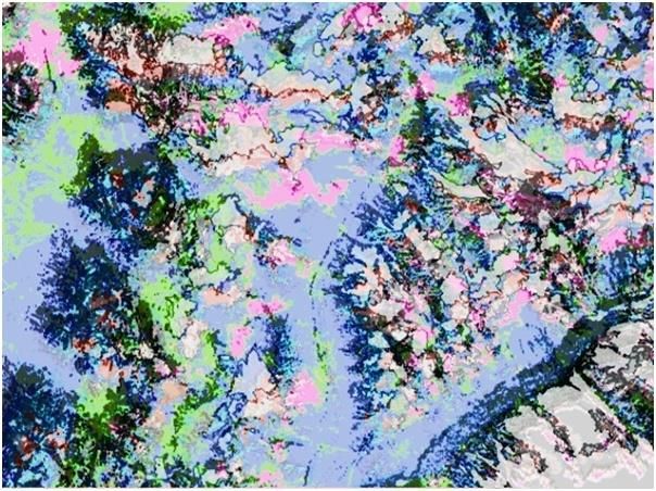
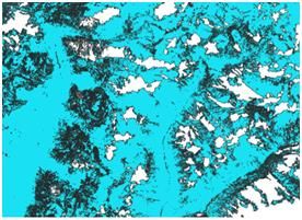
extensions are generated cpg, dbf, prj, shp and shx at the same directory.

3.3.5 Significant flood extent extraction

 The massive numbers of tiny polygons are generated during the process of
polygonizaion. They are representative of wet roads, wet roofs or swimming pools, dams or
reservoirs. They are not essentially representing the authentic flood extent while acting as
artificial water bodies. Also huge numbers of polygons directed a lengthy processing time
(about 7 to 8 hours) even the personal computer has 16GB RAM. In order to remove the
excess polygons the area is identified. After calculating the area of polygons, the same script
removes the polygons of below 500 sqm. Then it computes the buffer area for all features
using fixed distance. Buffered vector image in Figure 4 stored in the same directory for future
reference.

 Figure 4 Buffered vector

 The calculated tiny polygon areas of below 500 sqm in the premises of Matanuska
will be predicted other than artificial water bodies included as defined. This computes buffer
area for all features by fixed distance for flood occurrences. The major area covers indicated
in white colour are flooded areas. Vegetation indicated black and all other areas indicated by
light red for the sake of clarity.

3.4 Deep learning prediction

 The progresses involved in deep learning prediction using GBM are depicted in
Figure 5 that the Sentinel-2 data is pre-processed and ready for data extraction. The attributes

of generated Polygons are extracted for the prediction process step by step. The following
section clearly depicts the data manipulation.

 Figure 5 Flow of deep learning prediction

 Deep learning prediction involves the following steps as Dataset preparation, Result
Handling and performance evaluation. Dataset is prepared by the pre-processed Sentinel-2
images. Result handling is the process of conversion from the raster file into data frames from
the data science modules implemented in python. Ultimately the performance would be
calculated by its loss functions called Mean Squared Error (MSE), Root Mean Square Error
(RMSE) and log-loss.

3.4.1 Dataset preparation

 In a nutshell, preparation of a dataset is a collection of procedures that assists our
dataset more appropriate for deep learning. The Digital Flood Insurance Rate Map (DFIRM)
Dataset illustrates flood risk data and its following information utilized to expand the risk
information. The principal risk classifications might be implemented are the 1% of annual-
chance flood event, the 0.2 % annual-chance flood event, and areas of minimal flood risk.
DFIRM Database is generated from previously published Flood Insurance Rate Maps
(FIRMs), the flood based prediction is performed in the support of these databases and the
generated mapping information is frequently generated in the Federal Emergency
Management Agency (FEMA) with the geo-referenced earth based coordinate system.

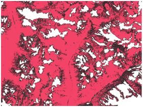
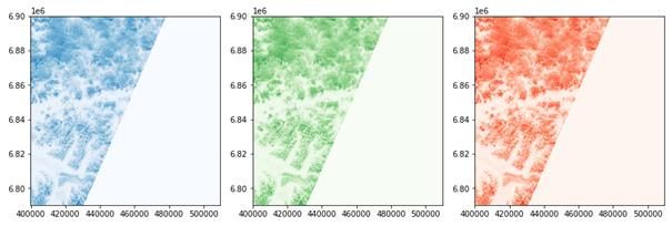
3.4.2 Extracting and handling the results

 In our work, the generated Shape file is checked whether it has UTF encoding or not.
Extracted the parameters from the shape file converted into data frame (geopandas), once the
right encoding format was found. The h2o performance function in python returns necessary
pre-computed performance metrics applied to the dataset for training/validation and also
cross validated based on model configuration. Above and beyond the utility functions that
return necessary metrics.

4. Performance evaluation

 A novel satellite raster dataset which will provide a brief land cover classification for
flood prediction of Matanuska River, Alaska in Figure 6 after processing the multiband image
through GBM with GPU of colab.

 Figure 6 Matanuska, Alaska (Google Map)

 The final dataset contains (27,000) labelled images with two different land cover
classes. The major difference compared to preceding datasets is that the currently obtained
one which can be a multi-spectral appearance in nature which covers spectral bands of
visible, shortwave infrared and near infrared art of spectrum. The part of coverage through
the bands of Sentinel-2 B is depicted in Figure 7. S2B_MSIL1C Multi-spectral band is

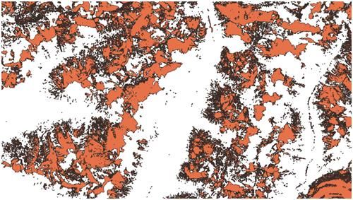
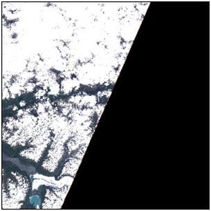
illustrated in Figure 8. True colour images of bands B2, B3 and B4 representation are
illustrated as Figure 9.

 Figure 7 Matanuska Sentinel-2 (S2B) coverage from Copernicus Open Access Hub

 Figure 8 S2B_MSIL1C Multi-spectral band

Figure 9 True colour images of bands B2, B3 and B4

 The prediction of the flood zone is identified based on the deep learning performance
evaluation. In this view, the distance vertically from y value, for every data point on the curve
fit that squares the value, typically defined MSE. Another quantity that can be determined is
RMSE. That is possibly the simply interpreted statistic, since it has the similar units as the
amount plotted on the vertical axis. Log-loss could also quantify the accuracy of a classifier
by penalising false classifications. Consequently the average of errors in each class defined as
Mean Per-Class Error found 0.

 MSE is the estimator that contains the procedure to estimate the errors which is
related to the error loss, it is computed using Eq. (3).

 1 2
 = ∑( − ̅ ) (3)
 
 =1

 where ̅ is the mean value of the event . The RMSE is a commonly used
measurement for the computation of dissimilarity within the values to compute the accuracy
and it is computed using Eq. (4).

 1 2
 = √ ∑( − ̅ ) (4)
 
 =1

 The log-loss function is the measurement of the dissimilarity within the probability
distribution from a group of events within the random variable; it is computed in Eq. (5)

 
 1
 ( ) = − ∑ log( ( )) + (1 − ) log(1 − ( )) (5)
 
 =1

 where N is the total amount of random variables, ( ) is the probability value of the
distribution event . MSE, RMSE, Log-loss also with predicted results plotted in Figure 10.

 Figure 10. Performance and error rate

4.1. GBM of flood zone prediction

 A deep learning model has been constructed by the GBM which typically follows a
forward learning ensemble method. It provides a valuable prediction with improved ability to
train on categorical variables. Also, worthy predictive results can be gained through
increasingly refined approximations. Figure 11 illustrates the gradient boosting models that
consist of the number of trees, internal trees, model size, depth values and leaves values.
GBM could be built using a forward stage-wise stabilized model by executing gradient
descent in function space. The same as gradient descent in parameter space iteration of each
element, the direction of the descent is given by its negative gradient of the loss function. A
regression tree model is fitted to forecast the negative gradient. Normally the squared error is
used as a replacement loss in obvious cases at each step.

Figure 11 Gradient Boosting Models

4.2. Maximum Metrics (Accuracies at their respective thresholds)

 Figure 12 projected the maximum metrics at their individual threshold with accuracy
will help us to probe the additional performance in our existing model. The value of
Maximum accuracy and the maximum specificity has reached the highest value, the other
parameters have the minimum value for the maximum threshold value.

 Figure 12 Accuracies and threshold

As for as our deep learning model is concerned for the flood zone identification best
accuracy could be found at good levels, the average threshold value is near 0.974.

4.3. Gains/ lift table

 The Gains/Lift values in Table 3 are used as predicted data to evaluate model
performance. The cumulative lift is calculated by gains. The accuracy from the model of
flood zone identification is evaluated according to the results when the model is and is not
used. The model could be saved for future access and conveniences.

 Table 3 Gain and Lifts

 Gains/Lift Table: Average response rate: 87.50 %, Avg score: 87.48 %
 Cumulative
 1.14286 1.14286 1.14286 1.14286 1.14286 1.14286 1.14286 1.14286
 lift
 Response
 1 0 1 1 1 1 1 1
 rate
 Score 0.99918 0 0.99917 0.99917 0.99917 0.99916 0.99916 0.99916
 Cumulative
 1 1 1 1 1 1 1 1
 response rate
 Cumulative
 0.99918 0.99918 0.99918 0.99917 0.99917 0.99917 0.99917 0.99916
 score
 Capture
 0.03759 0 0.01504 0.01128 0.09023 0.22181 0.3985 0.03008
 rate
 Cumulative
 0.03759 0.03759 0.05263 0.06391 0.15414 0.37594 0.77444 0.80451
 Capture rate
 gain 14.2857 -100 14.2857 14.2857 14.2857 14.2857 14.2857 14.2857
 Cumulative
 14.2857 14.2857 14.2857 14.2857 14.2857 14.2857 14.2857 14.2857
 gain

4.4. Variable importance and scoring history

 The variable importance computed from tree-based models also scores the history of
the model depicted in Figure 11. Study type, Object ID, Flood area ID and DFIRM ID are
taken as input variables. The GBM model gives highest priority to study type.

Figure 11 Variable importance

 This scoring history demonstrates the performance of the models through iterations
and illustrates the duration of each epoch. This history examined the overall performance of
the flood zone identification model in Figure 12.

 Figure 12. Scoring history

The predicted vector images for next five years can be obtained by the dataset converted back
to a shape file with the help of rasterio python in Figure 13.

 2021 2022

 2023 2024

 2025 2026

 Figure 13 Flood predictions on Matanuska, Alaska for six years (2021-2016)

 The cluster of images which are representing the flood prediction region of
Matanuska River, Alaska for the next six years is combined into a single image depicted in
Figure 14.

Figure 14. Combined view of flood level prediction for next six years (2021-2026)

 The cluster of images which are representing the flood prediction region of
Matanuska River, Alaska for the next six years is combined into a single image. These
collisions and threshold levels are obviously monitored and static indicators known as high
impact of the Matanuska river premises. There are several aspects played that work
simultaneously on the river for the rapid changes in significant ways. The impacts along the
river are hazardous because the flood will be probed in infrequent actions of natural factors.
All combined areas of flood are highly predicted for the next six years indicating the area in
which the precautionary measures should be taken indeed.

 As indicated by the outcomes accomplished in Section 4, the proposed strategy
emphatically improves the unwavering quality of flood orders for forthcoming five years in
Matanuska (Figure 13) where sand surfaces for the most part lead to solid overestimations of
the water degree. As can be seen in Figure 14, Matanuska as visualized can be utilized to
improve the after effects of the pooled flood covers determined by the Sentinel-2 high-
resolution images in this location. In this view, the uniqueness emphasizes on our proposed

framework the adaptability of the technique to other flood situations in parched zones. This
impression of our proposed work overcomes the constraint of existing methodologies [10],
[13], [14], [25], [40], [41] where the investigations just work on the conventional methods
based flood planning in dry and wet zones. Also the proposed framework reduces this
contrast when the flooding happens over all time low-back scattering sand surfaces.

5. Conclusion

 In this study, we have produced the predicted values of challenge in land cover
classification for the river in Alaska (Matanuska). We have prepared a novel high-resolution
dataset based on remotely sensed Sentrinel-2 raster bands. Earth observation program,
Copernicus has freely given the high quality raster images for accomplishing this task. There
are nineteen features used in the proposed dataset comprising 25245 rows of flood zone
information. We have analysed the geographical presentation of the thirteen dissimilar
spectral bands whereas B2, B3, B4 and B8 bands are used to analyse the flood region. The
above said features are extracted by giving raster inputs and the same has been processed by
GDAL and rasterio python and produced shapefile polygons. The extracted features have
been given in the deep learning framework supported by the Colab for prediction. As a result
of this appraisal, the prediction with accuracy of 97% represented the result by polygons with
its attributes. The novel dataset influenced real-world Earth science and scrutiny applications.
These all are the potential applications are land use and land cover change identification or
the enhancement of geographical maps. Subsequently, several data that can have a
considerable influence obtaining high-resolution Sentinel-2 data will lead to research in
analysing and predicting.

Declaration of interests

The authors declare that:

They have no known competing financial interests or personal relationships that could have
appeared to influence the work reported in this paper;

They have no financial interests/personal relationships which may be considered as potential
competing interests.

This statement is agreed by all the authors to indicate agreement that the above information is
true and correct.

References

[1]. S. Basu, S. Ganguly, S. Mukhopadhyay, R. DiBiano, M. Karki, and R. Nemani.
 Deepsat: a learning framework for satellite imagery. In Proceedings of the 23rd
 SIGSPATIAL International Conference on Advances in Geographic Information
 Systems, pp. 11-37, 2015.
[2]. B. Bischke, P. Bhardwaj, A. Gautam, P. Helber, D. Borth, and A. Dengel. Detection of
 Flooding Events in Social Multimedia and Satellite Imagery using Deep Neural
 Networks. In MediaEval, 2017.
[3]. B. Bischke, D. Borth, C. Schulze, and A. Dengel. Contextual Enrichment of Remote-
 Sensed Events with Social Media Streams. In Proceedings of the 2016 ACM on
 Multimedia Conference, pp. 1077–1081, 2016.
[4]. B. Bischke, P. Helber, J. Folz, D. Borth, and A. Dengel. Multi-Task Learning for
 Segmentation of Buildings Footprints with Deep Neural Networks. In arXiv preprint
 arXiv:1709.05932, 2017.
[5]. B. Bischke, P. Helber, C. Schulze, V. Srinivasan, and D. Borth. The Multimedia
 Satellite Task: Emergency Response for Flooding Events. In MediaEval, 2017.
[6]. M. Castelluccio, G. Poggi, C. Sansone, and L. Verdoliva. Land use classification in
 remote sensing images by convolutional neural networks. arXiv preprint
 arXiv:1508.00092, 2015.
[7]. G. Cheng, J. Han, and X. Lu. Remote sensing image scene classification: Benchmark
 and state of the art. Proceedings of the IEEE, 2017.
[8]. C. De Boor, C. De Boor, E.-U. Math´ematicien, C. De Boor, and C. De Boor. A
 practical guide to splines, vol. 27. Springer-Verlag New York, 1978.
[9]. W. Li, Q. Guo, and C. Elkan, “Can we model the probability of presence of species
 without absence data?” Ecography, vol. 34, no. 6, pp. 1096–1105, 2011.
[10]. J. Pekel, A. Cottam, N. Gorelick, and A. S. Belward, “High-resolution mapping of
 global surface water and its long-term changes,” Nature, vol. 540, no. 7633, pp. 418–
 422, 2016.
[11]. M. Feng, J. O. Sexton, S. Channan, and J. R. Townshend, “A global, high-resolution
 (30-m) inland water body dataset for 2000: First results of a topographic-spectral
 classification algorithm,” Int. J. Digit Earth, vol. 9, no. 2, pp. 113–133, 2016.
[12]. Y. Zhou et al., “Open surface water mapping algorithms: A comparison of water-
 related spectral indices and sensors,” Water, vol. 9, no. 4, Apr. 2017.

[13]. X. Yang and L. Chen, “Evaluation of automated urban surface water extraction from
 Sentinel-2A imagery using different water indices,” J. Appl Remote Sens., vol. 11, no.
 2, May 2017.
[14]. X. Yang, S. Zhao, X. Qin, N. Zhao, and L. Liang, “Mapping of urban surface water
 bodies from sentinel-2 MSI imagery at 10m resolution via NDWI-based image
 sharpening,” Remote Sens., vol. 9, no. 6, 2017.
[15]. Yao, F.;Wang, C.; Dong, D.; Luo, J.; Shen, Z.; Yang, K. High-resolution mapping of
 urban surface water usingZY-3 multi-spectral imagery. Remote Sens., vol. 7, pp.
 12336–12355, 2015.
[16]. Y. Yang and S. Newsam. Bag-of-visual-words and spatial extensions for land-use
 classification. In Proceedings of the 18th SIGSPATIAL international conference on
 advances in geographic information systems, pp. 270–279, 2010.
[17]. Ko, B.C.; Kim, H.H.; Nam, J.Y.; Lamberti, F. Classification of Potential Water Bodies
 Using Landsat 8 OL land a Combination of Two Boosted Random Forest Classifiers.
 Sensors, vol. 15, pp. 13763–13777, 2015.
[18]. Singh, K.; Ghosh, M.; Sharma, S.R. WSB-DA: Water Surface Boundary
 DetectionAlgorithm Using Landsat 8OLI Data. IEEE J. Sel. Top. Appl. Earth Obs.
 Remote Sens., vol. 9, pp. 363–368, 2016.
[19]. Xie, H.; Luo, X.; Xu, X.; Pan, H.; Tong, X. Automated Subpixel Surface Water
 Mapping from Heterogeneous Urban Environments Using Landsat 8 OLI Imagery.
 Remote Sens., vol. 8, 2016.
[20]. Zhou, Y.; Luo, J.; Shen, Z.; Hu, X.; Yang, H. Multiscale water body extraction in urban
 environments from satellite images. IEEE J. Sel. Top. Appl. Earth Obs. Remote Sens.,
 vol. 7, pp. 4301–4312, 2014.
[21]. Ben-Dor, E., Patkin, K., Banin, A., Karnieli, A., Mapping of several soil properties
 using DAIS-7915 hyperspectral scanner data - a case study over clayey soils in Israel.
 Int. J. Remote Sens., vol. 23, pp. 1043–1062, 2002.
[22]. Ben-Dor, E., Chabrillat, S., Dematte, J.A., Taylor, G.R., Hill, J., Whiting, M.L.,
 Sommer, S., Using imaging spectroscopy to study soil properties. Remote Sens.
 Environ., vol. 113, pp. 38–55, 2009.
[23]. A. Fisher, N. Flood, and T. Danaher, Comparing Landsat water index methods for
 automated water classification in eastern Australia, Remote Sens. Environ., vol. 175,
 pp. 167–182, 2016.

[24]. S. K. McFeeters, The use of the normalized difference water index (NDWI) in the
 delineation of open water features, Int. J. Remote Sens., vol. 17, no. 7, pp. 1425–1432,
 1996.
[25]. Y. Du, Y. Zhang, F. Ling, Q. Wang, W. Li, and X. Li, Water bodies’ mapping from
 sentinel-2 imagery with modified normalized difference water index at 10-m spatial
 resolution produced by sharpening the SWIR band, Remote Sens., vol. 8, no. 4, 2016.
[26]. B. N. Holben et al., AERONET—A federated instrument network and data archive for
 aerosol characterization, Remote Sens. Environ., vol. 66, no. 1, pp. 1–16, 1998.
[27]. Aerosol Robotic Network, accessed on Jul. 10, 2016. [Online]. Available:
 http://aeronet.gsfc.nasa.gov/
[28]. G. Thuillier et al., The solar spectral irradiance from 200 to 2400 nm as measured by
 the SOLSPEC spectrometer from the ATLAS and EURECA missions, Solar Phys., vol.
 214, no. 1, pp. 1–22, 2003.
[29]. B. Schmid et al., Comparison of columnar water-vapor measurements from solar
 transmittance methods, Appl. Opt., vol. 40, no. 12, pp. 1886–1896, 2001.
[30]. Ping Wang, Rudolf van Westrhenen, Jan Fokke Meirink, Sibbo van der Veen, Wouter
 Knap, Surface solar radiation forecasts by advecting cloud physical properties derived
 from Meteosat Second Generation observations, Solar Energy, vol. 177, pp. 47-58,
 2019.
[31]. Mokhtari, M.H., Deilami, K. & Moosavi, V. Spectral enhancement of Landsat OLI
 images by using Hyperion data: a comparison between multilayer perceptron and radial
 basis function networks. Earth Sci Inform, vol.13, no. 493–507, 2020.
[32]. Sheoran, S., Mittal, N. & Gelbukh, A. Analysis on application of swarm-based
 techniques in processing remote sensed data. Earth Sci Inform, vol. 13, pp. 97–113,
 2020.
[33]. Krishna, G., Sahoo, R.N., Pradhan, S. et al. Hyperspectral satellite data analysis for
 pure pixels extraction and evaluation of advanced classifier algorithms for LULC
 classification. Earth Sci Inform, no. 11, pp. 159–170, 2018.
[34]. T. Wan, H. Lu, Q. Lu, and N. Luo, Classification of high-resolution remote-sensing
 image using openstreetmap information, IEEE Geosci. Remote Sens. Lett., vol. 14, no.
 12, pp. 2305–2309, 2017.
[35]. G. Donchyts, J. Schellekens, H. Winsemius, E. Eisemann, and N. van de Giesen, A
 30m resolution surface water mask including estimation of positional and thematic

differences using Landsat 8, SRTM and Open- StreetMap: A case study in the Murray-
 Darling basin, Australia, Remote Sens., vol. 8, no. 5, 2016.
[36]. C. Sujatha and D. Selvathi, Connected component-based technique for automatic
 extraction of road centreline in high resolution satellite images, EURASIP J. Image
 Video Process., vol. 2015, no. 1, p. 8, 2015.
[37]. Ken T. Murata, Praphan Pavarangkoon, Atsushi Higuchi, Koichi Toyoshima, Kazunori
 Yamamoto, Kazuya Muranaga, Yoshiaki Nagaya, Yasushi Izumikawa, Eizen Kimura
 & Takamichi Mizuhara, A web-based real-time and full-resolution data visualization
 for Himawari-8 satellite sensed images, Earth Science Informatics, vol. 11, pp. 217–
 237, 2018.
[38]. Borhani, M. Consecutive spatial-spectral framework for remote sensing image
 classification, Earth Science Informatics, vol. 13, pp. 271–285, 2020.
[39]. Yanga A. Willie, Rajendran Pillay, L. Zhou & Israel R. Orimoloye, Monitoring spatial
 pattern of land surface thermal characteristics and urban growth: A case study of King
 Williams using remote sensing and GIS, Earth Science Informatics, vol. 12, pp. 447–
 464, 2019.
[40]. Y. Du, Y. Zhang, F. Ling, Q. Wang, W. Li, and X. Li, Water bodies’ mapping from
 sentinel-2 imagery with modified normalized difference water index at 10-m spatial
 resolution produced by sharpening the SWIR band, Remote Sens., vol. 8, no. 4, 2016.

[41]. Sandro M, Simon P and Kamila C, The Use of Sentinel-1 Time-Series
 Data to Improve Flood Monitoring in Arid Areas, Remote Sens., 10, 583, 2018

[42]. Ridley J. Strawbridge F, Card R, Phillips H, Radar backscatter characteristics of a
 desert surface. Remote Sens. Environ. 57, 63–78, 1996