The Donut Effect of Covid-19 on Cities - WFH Research

The Donut Effect of Covid-19 on Cities

 Arjun Ramani1 and Nicholas Bloom2

 May 21th 2021

Abstract: Using data from the US Postal Service and Zillow, we quantify the effect of Covid-
19 on migration patterns and real estate markets within and across US cities. We find two
key results. First, within large US cities, households and businesses have moved from the
dense central business districts (CBDs) towards lower density suburban zip-codes. We label
this the “Donut Effect” reflecting the movement of activity out of city centers to the suburban
ring. Second, while this observed reallocation occurs within cities, we do not see major
reallocation across cities. That is, there is less evidence for large-scale movement of activity
from large US cities to smaller regional cities or towns. We rationalize these findings by
noting that working patterns post pandemic will be primarily hybrid, with workers
commuting to their business premises typically 3 days per week. This level of commuting is
less than pre-pandemic, making suburbs relatively more popular, but too frequent to allow
employees to leave the cities containing their employer.

Contact: aramani3@stanford.edu, nbloom@stanford.edu,
JEL No. D13, D23, E24, J22, G18, M54, R3
Keywords: Covid, working-from-home, real-estate
Acknowledgements: We are grateful to Pete Klenow and Marcelo Clerici-Arias for helpful
discussions and to Saketh Prazad for excellent research assistance. We thank Nadia
Evangelou for help locating the USPS data and Yichen Su, Sitian Liu, Jean-Felix Brouillete,
Melanie Wallskog, Rose Tan, Franklin Xiao, Megha Patnaik, Eduardo Laguna, Nano
Barahona, and Nina Buchmann for comments on previous versions of this paper. We thank
Stanford University for financial support.

1
 Stanford University
2
 Stanford University, SIEPR and the NBER

 1

1 Introduction

Since the inception of the internet, many have predicted that working-from-home (WFH) would
rapidly grow and end the dominance of cities in America’s economic geography. Instead, the
opposite occurred. WFH gradually rose for the first two decades of the 21st century, but
American ‘superstar’ cities like New York and San Francisco also grew. In the past year, news
outlets have made similar predictions. The Atlantic postulated “the decline of the coastal
superstar cities” and the “rise of the rest” going as far as to say that “the next Silicon Valley is
nowhere.” To what extent are such theories true?

Our goal in this paper is to determine how Covid and the rise of WFH have affected migration
patterns and real estate markets within and across US cities. We pay particular attention to
Central Business Districts (CBDs), areas like Manhattan in New York with a high concentration
of business activity and population density. In theory, WFH enables an employee to live further
away from their place of work by reducing or eliminating commutes. For example, one could
more easily work a high-paying job based in New York City while living in a cheaper suburb or
even another state. Thus, the rise of WFH should reshape migration patterns and consequently
the demand for real estate across different locations. To test this theory, we measure real estate
rents and prices using data from the Zillow Group and migration patterns using the National
Change-Of-Address (NCOA) dataset from the United States Postal Service (USPS). 1 We draw
three main sets of findings from the data.

Our first result is that real estate demand as measured by rents or prices reallocates away from
major city centers towards lower density areas on the outskirts of cities in a phenomenon we call
the “donut effect”. 2 This alludes to the hollowing out of the city center and the rise of the
surrounding suburbs like the shape of a donut. Rental rates in the central business districts
(CBDs) of the largest 12 US metros have fallen almost 18 percentage points relative to the
change in the bottom 50% of zip codes by population density. 3 Similarly, home price growth in
CBDs have realized losses of around 12 percentage points compared to changes in such low-
density zip codes.

Migration patterns as measured by the USPS show a similar pattern of reallocation. CBDs of the
top 12 US cities have seen net population outflows cumulating to more than 15% of their pre-
pandemic population and business establishment outflows totaling more than 14% of their pre-
pandemic stock both relative to pre-pandemic trends. The bottom 50% of zip codes by density
have gained about 2% of their pre-pandemic stock for both population and businesses vs pre-
pandemic trend.

1
 Our data and replication code are available to other researchers at https://github.com/arjunramani3/donut-effect.
2
 We decided to label this as “Donut effect” rather than a “Doughnut effect” for brevity, noting the variations in
usage across American vs British English (traditionally American being the former and British the later).
3
 The donut effect is more pronounced in larger cities (See Figure 4). We therefore limit the baseline results to the
twelve largest Metropolitan Statistical Areas (MSAs) in the US by population which are New York, Los Angeles,
Chicago, Dallas, Houston, Miami, Philadelphia, Washington DC, Atlanta, Boston, San Francisco, and Phoenix.

 2

Our second result is that the donut effect is primarily large city phenomenon. Outside of the
twelve largest metro areas by population, we do not observe much price growth divergence or
difference in population outflow between the CBD and lower density zip codes. The donut effect
is more widespread when measured through rents but is still primarily a large-city phenomenon.
The top 12 cities as measured by population see the strongest donut effects, the next 13-50 cities
see small effects, while the remaining 51 to 365 cities see no effects.

Third, though we observe a within-metro reallocation in economic activity, we observe much
less between-metro reallocation in activity. Indeed, metro-level regressions show that price
growth was actually stronger in denser metros. Change-of-address data on the other hand show
some movement across metros from denser metros to sparser metros, but this movement is
quantitatively small relative to the within-metro movement from city centers to their suburbs.
Overall, this finding suggests that the rise of so-called “Zoom Towns”, smaller cities across
America that have been marketed as remote work hubs, may not represent a broader long-term
trend in the data. 4

To interpret our data, we build a simple spatial equilibrium model with two metro areas, each
containing a city center and a suburb. We introduce both hybrid-WFH and full-time WFH to the
model and find that hybrid-WFH generates predictions more in tune with the data than full-time
WFH. This is because hybrid-WFH allows employees to move further from their place of work,
such as from a city center to a surrounding suburb. But it does not allow an employee to move to
another metro area entirely because they must still commute to work on some days.

Our study relates to a growing literature on Covid, WFH, and real estate markets. A first strand
of papers looks at the impact of WFH during Covid. Several papers calculate the share of jobs
that can be done from home by occupation or industry (e.g., Dingel and Neiman (2020) and
Mongey, Pilossoph and Weinberg (2020)). Several other papers have calculated the share of
workers actually working-from-home during Covid including (Barrero, Bloom, and Davis
(2020), Brynjolfsson et al. (2020), DeFilipis et al. (2020), Bick et al. (2020)) or have surveyed
managers about remote work (Ozimek, 2020a). De Fraja, Matheson, and Rockey (2020) look at
the incidence of WFH across geographies in the UK. Finally, a set of papers examine how WFH
impacts productivity and find generally positive effects though there is substantial variation
across workers (e.g., Bloom et al. (2015) and Emmanuel and Harrington (2020)).

A second set of papers builds spatial equilibrium models to model the impacts of WFH.
Delventhal, Kwon, and Parkhomenko (2021)’s model finds that jobs move to city centers even as
residents themselves move away from cities. Behrens, Kichko, and Thisse (2021) find that the
demand for office space falls while the demand for living space increases, while Davis, Ghent,
and Gregory (2021)’s model finds that the elasticity of substitution between in-person work and
WFH has changed in favor of WFH. Previous papers have also examined how productivity
spillovers and amenities lead to clustering in cities, especially of skilled workers (e.g. Albouy
(2016), Diamond (2016), Gyouko, Mayer, and Sinai (2013)). Couture et al. (2019) examine how
amenities also respond to this clustering of workers, and Leamer and Storper (2014) discuss how
IT affects economic geography.

4
 See Florida and Ozimek (2021) in the Wall Street Journal for the full essay.

 3

The most similar papers to our work empirically examine how Covid has impacted real estate
and migration. Su and Liu (2020) find that the demand for housing in dense locations has fallen
relative to demand in less dense locations and build a general equilibrium model to explain these
phenomena. Gupta et al. (2021) similarly find a flattening of the bid-rent curve in the top 30 US
metros. They find larger effects in metros with more WFH or lower housing supply elasticity and
impute future rental growth implied by property price changes. Brueckner, Kahn, and Lin (2021)
also document the reduction in home price gradients throughout the pandemic and model how
WFH enables people to move to high-amenity locations. Rosenthal, Strange, and Urrego (2021)
examine commercial real estate rents and find a reduction in rents in density locations, while
Ling, Wang, and Zhou (2020) document a drop in commercial real estate prices in areas more
exposed to Covid. Couture et al. (2021) use cell-phone data and find an outflow of people from
New York City. Haslag and Weagley (2021) use cross-state moving data from a moving
company and find a movement of mostly high-income people to smaller, less costly cities.
Ozimek (2020b) find in survey data that remote work has increased the number of planned
moves with more than half of survey respondents looking for more affordable housing.

Our findings complement the previous findings while addressing several previously unexplored
questions. First, we utilize US Postal Service change-of-address data to measure migration flows
whereas previous research has used cell-phone data, which is more likely to contain temporary
moves, or moving company data, which is limited to cross-state moves. Second, we examine
heterogeneity across the full set of US metros whereas previous studies have focused on a
smaller subset or have not looked at heterogeneity. Third, we show that while people, businesses,
and real estate demand reallocate from city centers to suburbs within metros, there is a less
substantial reallocation across metros. We interpret this finding to be consistent with a post-
Covid equilibrium of hybrid WFH as opposed to full-time WFH.

The rest of our paper is organized as follows: Section 2 describes our data and Section 3
documents our main results for both real estate markets and migration patterns. Section 4
outlines a simple model of both hybrid and full-time WFH and Section 5 concludes. We leave
robustness checks, additional charts, and the full model derivation for the Appendix.

2 Data

2.1 Zillow Price Indices

We use Zillow’s Observed Rental Index (ZORI) to measure changes in residential property
rental rates at the zip code and MSA levels. The rent index is constructed by tracking rent
changes for properties that remain listed across multiple periods. This repeated-rent methodology
is similar to repeat-sales methodologies used to construct price indices as in Wallace and Meese
(1997). In order to adjust for potential bias due to compositional shifts in listed properties, Zillow
reweights properties based on construction year, structure type, and rental year. Currently, ZORI
is only provided for the 100 largest US metros.

We also use Zillow’s Home Value Index (ZHVI) to measure changes in residential property
values at the zip code and MSA levels. The level of the price index is calculated by taking an

 4

average of Zillow’s Zestimate across all single-family homes in a given geographic area. The
growth in the price index is calculated by taking the value-weighted price appreciation of all
properties in a given geography. Zillow value-weights in order to capture the growth of the
overall value of the housing market. The Zestimate is supposed to be a real-time reflection of
property’s value. Zillow employs a hedonic model to estimate home values for periods in which
a property does not sell. The ZHVI is offered for almost the full universe of US metro areas. 5

2.2 USPS National Change of Address (NCOA) Dataset

To directly observe migration patterns, we utilize the United States Postal Service’s National
Change of Address (NCOA) dataset. We submitted a Freedom of Information Act (FOIA)
request to obtain zip code-month level inflow and outflow data for the universe of US zip codes
over the last four years. 6 There are multiple types of change of address requests. To construct our
measure of population inflows and outflows, we multiply the number of household change-of-
address requests by 2.5, the mean household size in the US, and add the number of individual
change-of-address requests. Because the USPS does not specify whether household moves are
exclusive of single-person households, we conservatively report results using the average
household size value that includes single-person households of 2.5. Using the average size of
non-single-person households, 3.2, strengthens the main results. 7

2.3 Working from home (WFH) exposure

We construct a zip code level measure of the share of jobs that can be done from home (WFH
exposure). An important difference from other studies is our measure uses the work industries
for the residents of zip codes as opposed to the business located in the zip code. This enables us
to more directly observe the exposure of a zip code to current residents changing their housing
demand for their current place of residence in response to the pandemic and WFH. We obtain the
job industry distribution for residents across US zip codes from the LEHD Origin-Destination
Employment Statistics (LODES) at the US Census Bureau 8. LODES data is available at the
census block level so we crosswalk to the zip code level. Finally, we merge the LODES data
with Dingel and Neiman (2020)’s data on the share of jobs that can be done from home at the 2-
digit NAICS level.

2.4 Central Business Districts (CBDs)

We map zip codes to their corresponding metro area’s central business district (CBD) using data
from Holian (2019). The paper compares several different sources and methods for defining
CBD coordinates and concludes that the 1982 Census of Retail Trade’s official coordinates best
fits the point of maximum agglomeration in a city. Since the 1982 Census of Retail Trade only
defines CBD coordinates for 268 metros, we define the CBDs for remaining metros using a

5
 More on the index methodologies employed by Zillow can be found at https://www.zillow.com/research/data/
6
 A summarized version of the USPS data for recent years is now available at:
https://about.usps.com/who/legal/foia/library.htm
7
 Household size data is from the US Census Bureau: https://www.census.gov/data/tables/time-
series/demo/families/households.html
8
 See https://lehd.ces.census.gov/data/

 5

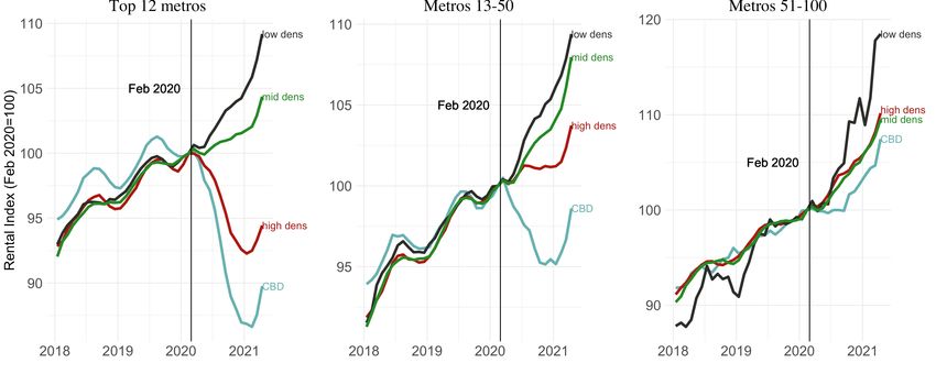
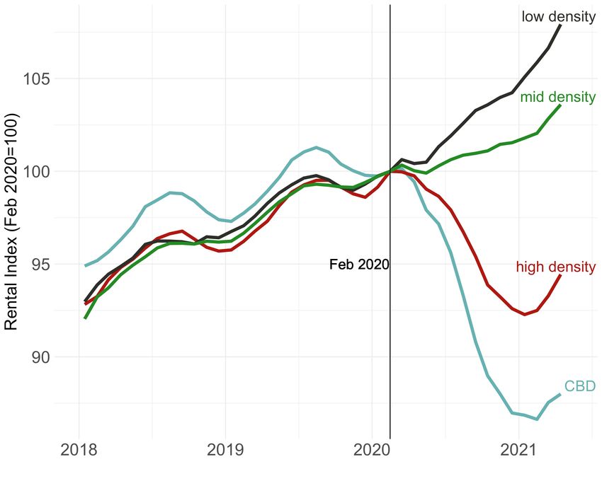
city’s City Hall – for metros where both exist, the City Hall coordinates generally track the 1982
Census CBD coordinates. We define the area of a CBD to contain all zip codes with centroids
within two kilometers of the CBD coordinates. The main results are robust to alternate CBD
radius distances from 1-10 kilometers.

3 Results

Our primary goal in this section is to characterize changes in migration patterns and real estate
markets both within and across US cities since the advent of Covid-19. We focus on zip-code
level factors that mediate the impact of Covid on real estate markets and migration patterns
including population density, distance of the zip code from the CBD, and the ability for residents
of the zip code to WFH.

3.1 Documenting the donut effect in real estate markets
Figure 1 shows the headline finding of a “donut effect” for the largest 12 US metros in the
residential rental market. We plot a population weighted-average of zip code level rental indices
bucketed into four groups: the central business district (CBD) and three groups of zip codes
grouped by population density. 9 Here and elsewhere, the three groups are given by high = top
10%, mid = 50-90th percentile, and low = 0-50th percentile. For rental rates and home values
there is a parallel trend of gradual growth across groups in the years preceding the Covid shock.
The parallel trend suggests that post February 2020 divergence in outcomes across the four
groups of zip-codes is a result of the impact of the pandemic.

After the Covid shock, we see a substantial divergence between the CBD and low-density
groups. Indeed, the difference in rent growth (Figure 1a) between the CBD and the low-density
group is approximately 20 percentage points by Jan 2021. The rental indices display a striking
drop starting in March 2020 that aligns with the start of Covid lockdowns and the shift to WFH
in the US. Though the rental indices have started to increase across groups since Feb 2021 due to
the reopening, the rental growth divergence has persisted. 10

9
 We normalize all indices to Feb 2020=100 after aggregating within each group. We aggregate first and then
normalize because then the price growth of our aggregated index is weighted both by population (a proxy for the
number of housing units) and the typical home value in a region (the level of the home value index). This approach
allows us to capture the growth of the overall housing market in a region and is similar to how Zillow constructs its
home value index. See Hryniw (2019) for more details on how Zillow value-weights in its index construction. As a
robustness check, we try normalizing each index to Feb 2020=100 and then taking a population-weighted average
across zip codes, which removes the value-weighting (See Appendix A3) The pattern of rent growth divergence and
price growth divergence post-Covid is generally preserved though the effect is smaller for prices. The smaller effect
absent value-weighting can be rationalized by noting that high-value regions likely suffered greater shocks since
individuals who can WFH are generally skilled high-income workers (Althoff et al., 2020).
10
 Here, we draw an inference from rental or price movements to a shift in demand for a location by making the
assumption that housing supply is inelastic in the short-run. This assumption may be less true in the longer-run
because real estate developers can respond to changes in demand, but there is some evidence that even over longer
time horizons housing supply is inelastic. For example, Green, Malpezzi and Mayo (2005) show that when demand
falls, the market cannot easily reduce the quantity of housing available because housing is durable. This asymmetric
nature of housing makes the supply curve especially downwardly inelastic. Zoning restrictions and geographic
constraints such as the fixed supply of land can also make the supply curve upwardly inelastic, though this varies
substantially across the country (Saiz, 2010)

 6

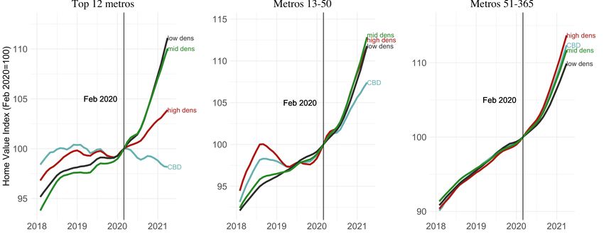
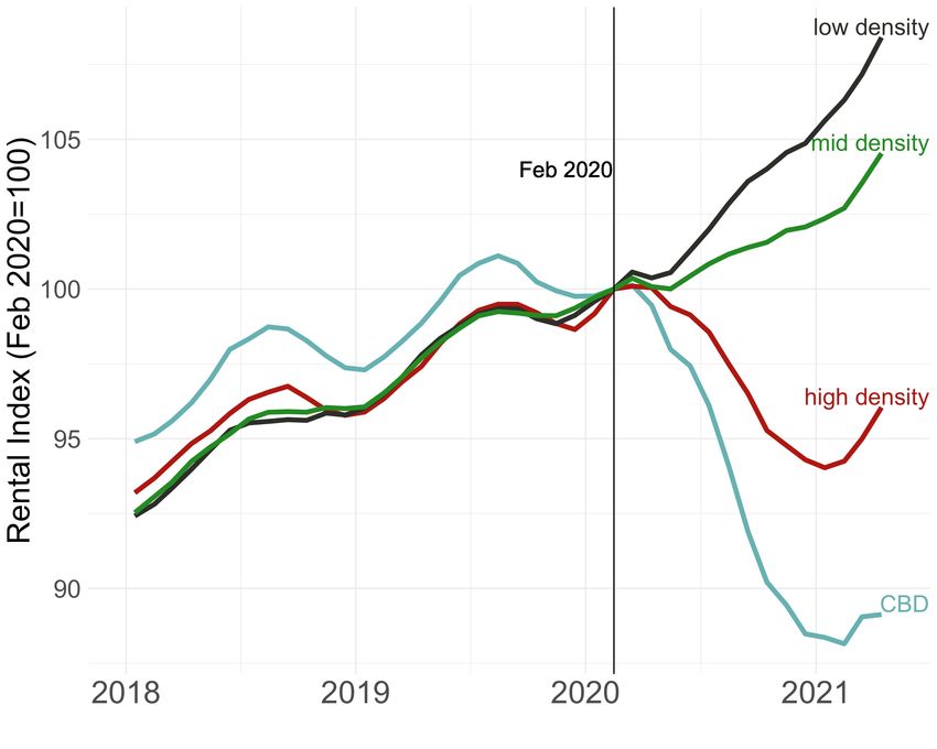
Residential property prices show a similar divergence after the pandemic (see Figure 1b) as
measured by Zillow’s home value index. After February 2020 the CBD and high-density group
diverge substantially from the mid and low-density group. The price growth gap reaches almost
15 percentage points by March 2021. The smaller difference in the level of price growth
compared to the rental growth indicates that the market expects the magnitude of the gap in rent
growth to fall, as indeed they appear to have started to do after February 2021. 11

Though there is reallocation in demand across density groups, it is worth noting that Covid has
also increased demand for housing in the aggregate by both increasing the demand for space
(Emmanuel and Harrington, 2020), and also making the cost of home-financing cheaper (Zhao,
2020). This may explain part of the upward trend across series for home prices compared to
rents.

To determine that factors that explain the donut effect, we run zip-code level regressions with
MSA fixed effects of the percent change in rent or price index from the Feb 2020 to Feb 2021 on
a set of zip-code level characteristics as specified in the following equation.

 % Δ , = + 1 %Δ , −1 + β2 ln + 3 ln _ + + (1)

Here, i indexes the zip code, m indexes the MSA, and % Δ is calculated by using the arc-
percentage change methodology from Davis, Haltiwanger, and Schuh (1996). This method takes
the percent change over the midpoint of the start and end-point values. 12

As seen in Table 1, population density and the share of residents who can WFH have negative
coefficients whereas distance from CBD has a positive coefficient. Columns (1) to (4) of table 1
show rents fall relatively more in zip-codes with greater density, greater WFH share, and lesser
distance to the CBD. These findings, which show the donut effect story for rent growth changes,
are broadly in line with other research and popular narratives around the impact of Covid on real
estate. 13

In columns (5) to (8) of Table 1, we show the results of the same set of regressions as columns
(1) to (4) except with the percent change in home value index as the dependent variable.
Interestingly, the WFH coefficient becomes insignificant after the introduction of density and
distance to CBD to the regression. One possible explanation for this is that WFH affects the
demand for housing on two margins. On the extensive margin, WFH may enable residents to
leave a zip code reducing the total number of home buyers or renters. On the intensive margin,
WFH may increase the demand for housing space perhaps due to increased time spent at home or
the need for home office space. The distance to CBD coefficient is positive and significant

11
 Home values are forward looking in that they measure both current demand and future expected demand for a
property. Thus, the 15-point gap suggests that a large portion of the divergence in price change will persist. To
check whether out findings are specific to the Covid-19 pandemic relative to past macroeconomic shocks, we
reproduce the main home values figure for both Great Recession and 9/11 in Appendix A4. Both shocks do not
produce divergence between regions showing the uniqueness of the Covid shock.
12
 Defined as dXt=(Xt-Xt-1)/(0.5×Xt+0.5×Xt-1)
13
 We tried including total Covid deaths per capita since the start of the pandemic as a control and find broadly
similar results.

 7

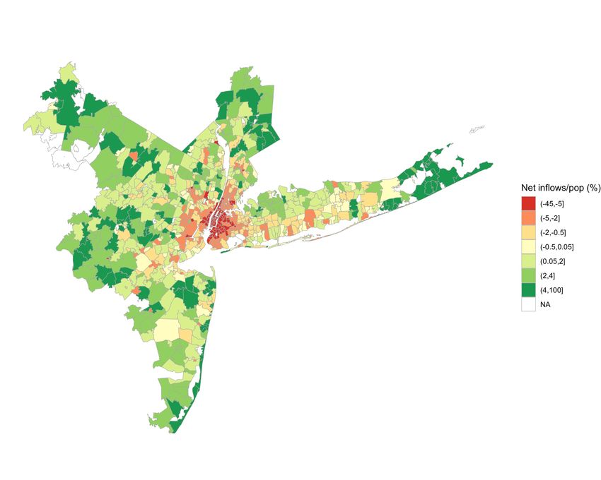
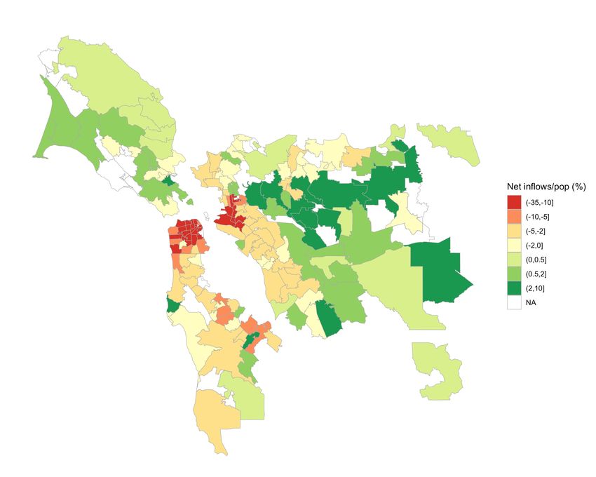
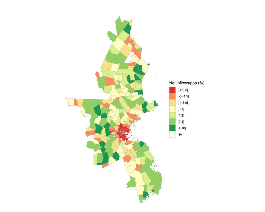
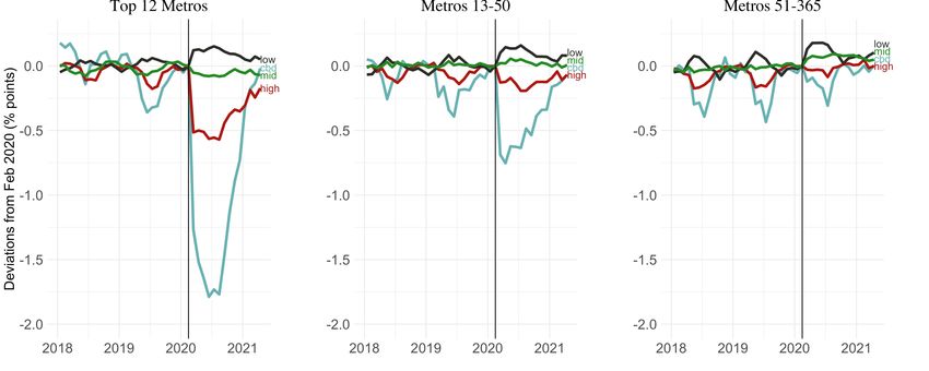
indicating relative price appreciation in zip codes further away from the city center. In general,
results are consistent with the donut effect: the rise of WFH has made dense areas near city
centers less attractive relative to the suburbs.

3.2 The donut effect exists in migration flows for people and businesses

Figure 2 panel A uses USPS change of address data to show the now-familiar story of
populations reallocating from CBDs to less dense zip codes within the largest metros in the US. 14
The outflows from CBDs are especially striking. Monthly population outflows (Figure 2a)
increase to almost 2% of the pre-Covid population for the CBDs of the 12 largest US metros. In
fact, since March 2020, the net population outflows versus their pre-pandemic trend for the top
12 metro CBDs has cumulated to 15% (see Figure A6). 15 These values highlight that the
pandemic-induced population flows are quantitatively material in terms of overall city-center
density.

Panel B of Figure 2 shows monthly net business establishment inflows based on change of
address requests as a share of the pre-Covid establishment stock. Business flows are broadly
similar to those of population flows but have a much sharper initial drop. Business outflows from
the top 12 CBDs versus pre-pandemic trends from Feb 2020 to Feb 2021 cumulate to around
14% of stock (Figure A6).

Figure 3 displays heat maps of the cumulative net population inflow from Feb 2020 to Feb 2021
as a percent of pre-Covid population for the New York metro area (Panel A) and the San
Francisco Bay Area metro area (Panel B). The heat maps show a striking pattern of outflows
from the dense central city areas of lower Manhattan (in New York) and San Francisco and
Oakland (in the Bay Area) towards the suburbs. Similar example maps for Boston and Los
Angeles in Appendix A7 reveal similar flows of population out from city centers to suburban
areas.

To investigate the factors driving population flows, we run regressions of a similar specification
to Equation 1 (which examined real-estate prices) except with cumulative net flows as a percent
of stock from Feb 2020 to Feb 2021 as the dependent variable:

 % Δ , = + 1 %Δ , −1 + β2 ln + 3 ln _ + + (2)

As we see in Table 2 columns (1) to (4) that net flows are strongly related to distance to the
CBD, density and WFH exposure.

Table 2 columns (5) to (8) shows the results of similar regressions for cumulative net inflows of
business establishments as a percent of total stock as the dependent variable. The regressions
14
 As a basic data check, Appendix A3 confirms a positive relationship between net population flows and residential
rental and price growth for zip codes in the 12 largest US metros.
15
 To adjust for the pre-pandemic trend, we take the difference in monthly flow with the flow level in Feb 2020
before cumulating. An alternative measure of the impact of the pandemic is to simply look at the total change in
population and businesses as a share of their stock since February 2020 in the CBD. Using this approach, we find
that the reduction in population is 18% and the reduction in businesses addresses is 14%. The larger population
outflows using this approach highlight that there were pre-existing outflows from CBDs before the pandemic.

 8

broadly confirm the donut effect pattern: density and WFH share have negative coefficients and
distance to CBD has a positive coefficient.

3.3 Heterogeneity across cities

How does the donut effect vary across cities? Figure 4 examines the donut effect in metros
outside the top 12 metros, finding little residential price growth dispersion. There is some
evidence that CBDs see slower price appreciation in cities ranked 13 to 50, but nothing in the
remaining cities ranked 51 to 365 by size. Figure 5 shows heterogeneity in the donut effect
across metros as measured by population flows, revealing a similar result. A clear drop in
population flows in the CBDs of the largest 12 US cities, a milder drop in cities sized 13 to 50,
and no impact in cities 51 to 365. 16 We see in Figure A1 in the appendix a similar result for rents
– a strong donut effect in the largest 12 cities, a milder effect in cities sized 13 to 50, and little
impact in the remaining cities ranked 51 to 365.

What explains variation in the donut effect across cities? As seen in the previous results, zip-
codes with a greater WFH share take bigger hits so if larger metros have greater WFH shares in
their city centers then we should expect such cities to have larger donut effects. Indeed, Althoff,
Eckert, Ganapati, and Walsh (2020) show that America’s largest cities have the highest
concentration of skilled service workers in industries like tech and finance who can WFH.
Furthermore, the incentive to relocate one’s home when given the option to work-from-home
may be greater in higher-priced locations which also tend to have greater population density.

These findings can be rationalized by thinking of WFH as a technology that mitigates traditional
agglomeration forces. Such forces have driven skilled workers to cluster near city centers
pushing up population density and price levels (see e.g. Glaeser and Gottlieb (2009) and
Diamond (2016)). Thus, cities with a greater share of residents who can WFH and high
population density which contributes to higher housing prices are more vulnerable to changes
from Covid-induced WFH.

3.4 Within-metro vs between-metro reallocation of economic activity

Several recent news articles have hypothesized a flight from expensive dense cities like New
York and San Francisco to less expensive areas like Austin or Miami. In this section, we test this
hypothesis by examining the relationship between metro-level population density and both home
price changes and migration patterns post-Covid. A key feature of our analysis is to compare the
within-metro relationship between population density and either housing prices or migration
flows with the between-metro relationship.

Figure 6 shows three zip code-level binscatters of the percent change in home value index (Panel
A), population (Panel B), or business establishment stock (Panel C) plotted against population
density after controlling for the pre-Covid trend. We include MSA fixed effects to show the
within-metro relationships. Similar to Sections 3.1 and 3.2, the three plots show a clear
reallocation of real estate demand, people, and business establishments away from high density
zip codes and CBDs towards lower density zip codes further from the city center.

16
 There is also evidence of CBD seasonality in the data, with populations falling in the summer.

 9

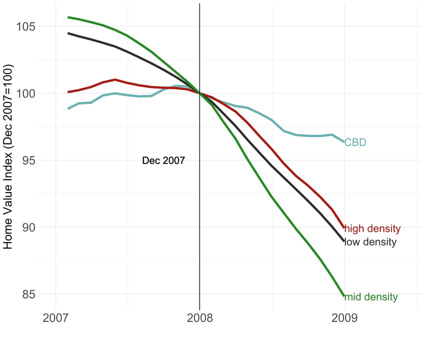
Figure 7 plots the same three figures as Figure 6, except at the metro-level instead of the zip code
level. The figures are on the same scale and have the same controls, except Figure 7 has metro-
fixed effects. Thus, Figure 7 examines changes between metros rather than within metros. All
three regression lines show flatter slopes compared to the within-metro binscatters. In fact, the
metro-level home price plot shows a positive relationship between home price changes and
metro-level population density. The flatter slopes indicate that the within-metro reallocation of
economic activity is stronger than the between-metro reallocation. Furthermore, the positive
relationship between density and home price changes at the metro-level suggests that real estate
market expect denser metros to perform well in the longer-term.

There are several interpretations of this data. First, many of the cross-city moves during the
pandemic may prove to be temporary. As cities reopen, residents may move back to their pre-
Covid metro areas, though perhaps slightly further away from the city center than their previous
residences.

A second explanation is that large dense metros typically have a high share of workers in
industries like tech and finance, which have grown as a share of GDP during Covid. Thus, some
of the price growth in previously expensive metros may be due to an income effect. For example,
Covid has induced a reallocation of economic activity towards the software industry (Barrero,
Bloom, and Davis, 2020b), which may have disproportionately benefited the incomes of both
previous and new residents of the suburbs of technology-heavy cities like San Francisco and
New York.

Third, the individuals who are moving to large metro suburbs may be spending a greater share of
income on housing (and are wealthier). Since large metros have seen more city-to-suburb
movement than small metros, the increased spending on housing for these newly suburban
dwellers could explain the metro-level price growth. Furthermore, large metros tend to have a
greater share of residents who can WFH, and Stanton and Tiwari (2021) find that home workers
spend a greater share of income on housing then non-homeworkers. Thus, the increase in WFH
in large metros could also contribute to metro-level price growth. Our view is that all three
explanations may be at play and estimating their relative magnitudes is a subject for future
research.

4 Model

In this section, we describe the basic features of a simple spatial equilibrium model in order to
rationalize the key findings of the empirical section. The model is loosely inspired by the one-
city two-location model proposed by Liu and Su (2020) but with a number of key differences.
First, we add two more locations in order to model the between vs within dynamics documented
in the data. Second, we add in productivity and wage differences to differentiate between the two
metros and modify the functional forms of the utility function and housing supply curves.
Finally, we simulate both a hybrid-WFH shock and a full-time WFH shock. Overall, the purpose
of this model is to illustrate how both the within-metro and between-metro population flow
dynamics change under very simple assumptions on the nature of WFH.

 10

4.1 Model setup

Consider two metro areas, one large and one small. Each metro has a city center and a suburb
giving a total of four locations. Locations are indexed as follows: big metro city center = 1, big
metro suburb = 2, small metro city center = 3, small metro suburb = 4. Homogeneous individuals
choose a location to maximize utility, which is a function of wages, amenities, commute costs,
and housing rents.

Utility is Cobb-Douglas in wages, commute costs, amenities, and rents.

 − 
 = − (3)

We let productivity and amenities vary by location. Rents have a constant elasticity with respect
to population level. In Appendix B1, we describe the model ingredients in more detail. We also
solve for the spatial equilibrium under three scenarios: (i) no WFH, (ii) hybrid WFH, and (iii)
full-time WFH.

4.2 Commute costs

We simulate three states of the world based on the level of their commute costs shown in the
table below.

 Average commute costs
 Large metro Small metro
 City center Suburb City Center Suburb
 No WFH 1 1 
 Hybrid WFH 
 Full-time WFH 0 0 0 0

Here, > 1 represents the cost of commuting from suburb to city relative to a baseline cost of 1
for within-city commuting. 1 − represents the share of days worked from home in the hybrid
setting. Therefore, we multiply commute costs by to obtain the new commute cost under
hybrid WFH. Survey data from Barrero, Bloom and Davis (2020) indicates that employees who
will WFH post pandemic (about half of all employees) will spend 2 days a week at home post-
pandemic, implying ≈ 0.6.

4.3 Comparative statics

To solve for the spatial equilibrium, we equate utility across our four locations since we have
homogenous individuals. We derive solutions for the difference in population both between each
city center and its corresponding suburb as well as between the two metro regions in Appendix
B1. Comparing these population differences yields the following comparative statics which can
be interpreted as the net population flow from after the introduction of the WFH technology.

 11

Within-metro reallocation Between-metro reallocation

 WFH model Δ( 1 − 2 ) + Δ( 3 − 4 ) Δ( 1 + 2 − 3 − 4 )

 (1 − )4 ( − 1)
 Hybrid WFH 0
 
 4 ( − 1) 2( 1 − 2 )
 Full-time WFH
 
The relative metro-level populations are pinned down solely by productivity and amenities which
do not change with partial telework. Therefore, though there is positive between-metro
reallocation with full WFH proportional to underlying productivity differences, there is no
between-metro reallocation under hybrid WFH. In general, hybrid WFH generates qualitative
predictions that better match the patterns seen in the USPS and Zillow home values data than
does full WFH.

In particular, the degree of within-metro reallocation under the hybrid WFH scenario is less than
that of full-time WFH scenario. In particular, the parameter π, which is the share of days worked
in the office, governs the extent of the reallocation. A smaller value of π, or more remote work,
leads to more reallocation. This pattern matches the observed pattern of a quantitatively more
negative relation between density and both population outflows within metros relative to across
metros.

5 Conclusion

Covid-19 has induced substantial change to the organization of work. In this paper, we aim to
answer the question of how such changes have impacted the economic geography of the US both
in the short and long-term.

This paper contributes several findings to the growing literature on Covid-19, working-from-
home, migration, and real estate markets. First, we establish evidence supporting a "donut effect"
in migration patterns and real estate markets. About 15% of population and 14% of business
establishments appear to have moved out of the centers of large cities over the first year of the
pandemic. Much of this movement has been to the suburbs which have seen a price growth
divergence from their city centers of almost 15 percentage points.

Our second contribution is identifying heterogeneities in how migration patterns and real estate
markets have responded across almost the full set of US metros. There is clear evidence of a
donut effect in the 12 largest US cities, some evidence in the next 13 to 50 sized US cities, and
no evidence in smaller cities beyond this. This pattern suggests that the largest US cities have

 12

seen the sharpest movement of economic activity out of city centers into the surrounding
suburbs.

Our third contribution is showing that the within-metro reallocation of economic activity, i.e. the
donut effect, is stronger than the between-metro reallocation of activity from dense metros to less
dense metros. To interpret this finding, we build a simple spatial equilibrium model with two
metro areas, each with a city center and a suburb. Our model generates qualitative patterns that
better match the empirical data under the hybrid-WFH scenario compared to the full-time WFH
scenario. We take this as evidence that post-pandemic, work will be primarily hybrid, with
workers commuting to their business premises a couple days a week. This is less than pre-
pandemic, making suburbs relatively more popular, but too frequent to allow employees to leave
the cities containing their employer.

This paper suggests several avenues for additional research. First, this paper abstracts away from
the heterogeneity of WFH ability across the wage distribution. Since WFH is highly correlated
with high-wage workers, the reallocation of high-wage workers from city centers is likely to
disproportionately impact consumption of city services and amenities like restaurants. An open
question is to estimate the magnitude of the impact on consumption amenities. A second open
question is how the political economy equilibrium may change after urban flight. Cities like New
York and San Francisco have a high degree of supply constraints on housing which has reduced
populations. If cities respond to falling tax revenue by lifting constraints on new housing, then a
different long-term equilibrium may emerge.

 13

References

Albouy, David, 2016. "What are cities worth? Land rents, local productivity, and the total value
 of amenities." Review of Economics and Statistics 98, no. 3: 477-487.
Althoff, Lukas, Fabian Eckert, Sharat Ganapati, and Conor Walsh, 2020. "The City Paradox:
 Skilled Services and Remote Work," CESifo Working Paper No. 8734.
Barrero, Jose Maria, Nicholas Bloom, and Steven J. Davis, 2021. “Why working from home will
 stick,” NBER Working Paper 28731.
Barrero, Jose Maria, Nicholas Bloom, and Steven J. Davis, 2020. “Covid-19 is also a reallocation
 shock,” NBER Working Paper 27137.
Behrens, Kristian, Sergey Kichko, and Jacques-François Thisse, 2021. "Working from home:
 Too much of a good thing?." CESifo Working Paper No. 8831.
Bick, Alexander, Adam Blandin, and Karel Mertens, 2020. "Work from home after the Covid-19
 Outbreak,” Federal Reserve Bank of Dallas Working Paper.
Bloom, Nicholas, James Liang, John Roberts, and Zhichun Jenny Ying, 2015. "Does working
 from home work? Evidence from a Chinese experiment," The Quarterly Journal of
 Economics 130, no. 1: 165-218.
Brueckner, Jan, Matthew E. Kahn, and Gary C. Lin, 2021. “A New Spatial Hedonic Equilibrium
 in the Emerging Work-from-Home Economy?” NBER Working Paper 28526.
Brynjolfsson, Erik, John J. Horton, Adam Ozimek, Daniel Rock, Garima Sharma, and Hong-Yi
 TuYe, 2020. “COVID-19 and remote work: An early look at US data,” NBER Working
 Paper 27344.
Ciccone, Antonio, and Robert E. Hall, 1996. “Productivity and the density of economic activity,”
 The American Economic Review, 54-70.
Couture, Victor, Jonathan I. Dingel, Allison Green, Jessie Handbury, and Kevin R. Williams,
 2021. "JUE Insight: Measuring movement and social contact with smartphone data: a real-
 time application to COVID-19." Journal of Urban Economics: 103328.
Couture, Victor, Cecile Gaubert, Jessie Handbury, and Erik Hurst, 2019. “Income growth and the
 distributional effects of urban spatial sorting.” NBER Working Paper 26142.
Davis, Morris A., Andra C. Ghent, and Jesse M. Gregory, 2021. “The Work-at-Home
 Technology Boon and its Consequences,” NBER Working Paper 28461.
Davis, Steven J., John Haltiwanger, and Scott Schuh, 1996. “Job creation and job destruction,”
 MIT Press.
DeFilippis, Evan, Stephen Michael Impink, Madison Singell, Jeffrey T. Polzer, and Raffaella
 Sadun, 2020. “Collaborating during coronavirus: The impact of Covid-19 on the nature of
 work,” NBER Working Paper 27612.
Delventhal, Matthew J., Eunjee Kwon, and Andrii Parkhomenko, 2021. "JUE Insight: How do
 cities change when we work from home?" Journal of Urban Economics: 103331.
Diamond, Rebecca, 2016. “The determinants and welfare implications of US workers’ diverging
 location choices by skill: 1980-2000,” American Economic Review 106, no. 3: 479-524.
Dingel, Jonathan I., and Brent Neiman, 2020. "How many jobs can be done at home?" Journal of
 Public Economics 189: 104235.
Emanuel, Natalia, and Emma Harrington, 2020. “‘Working’ remotely?: Selection, treatment and
 the market provision remote work”. Harvard mimeo.
Florida, Richard and Ozimek, Adam, 2021, “How Remote Work Is Reshaping America’s Urban
 Geography,” Wall Street Journal, 5 March.

 14

Garcia, Joaquin Andres Urrego, Stuart S. Rosenthal, and William C. Strange, 2021. "Are City
 Centers Losing Their Appeal? Commercial Real Estate, Urban Spatial Structure, and
 COVID-19,” Working Paper.
Glaeser, Edward, and Joshua Gottlieb, 2009. "The wealth of cities: Agglomeration economies
 and spatial equilibrium in the United States," Journal of economic literature 47, no. 4: 983-
 1028.
Green, Richard K., Stephen Malpezzi, and Stephen K. Mayo, 2005. "Metropolitan-specific
 estimates of the price elasticity of supply of housing, and their sources." American
 Economic Review 95, no. 2: 334-339.
Gupta, Arpit, Vrinda Mittal, Jonas Peeters, and Stijn Van Nieuwerburgh, 2021. “Flattening the
 curve: Pandemic-induced revaluation of urban real estate,” NBER Working Paper 28675.
Gyourko, Joseph, Christopher Mayer, and Todd Sinai, 2013. "Superstar cities." American
 Economic Journal: Economic Policy 5, no. 4: 167-99.
Haslag, Peter H., and Daniel Weagley, 2021. "From LA to Boise: How Migration Has Changed
 During the Covid-19 Pandemic," Available at SSRN 3808326.
Holian, Matthew. J., 2019. “Where is the City's Center? Five Measures of Central
 Location,” Cityscape, 21(2), 213-226.
Hryniw, Natalia, 2019. “Zillow Home Value Index Methodology, 2019 Revision: Getting Under
 the Hood,” Zillow Group.
Leamer, Edward E., and Michael Storper, 2014. "The economic geography of the internet age."
 In Location of international business activities, pp. 63-93. Palgrave Macmillan, London.
Lee, Sanghoon, and Jeffrey Lin, 2018. "Natural amenities, neighbourhood dynamics, and
 persistence in the spatial distribution of income." The Review of Economic Studies 85, no. 1:
 663-694.
Ling, David C., Chongyu Wang, Tingyu Zhou, 2020. A First Look at the Impact of COVID-19
 on Commercial Real Estate Prices: Asset-Level Evidence, The Review of Asset Pricing
 Studies, 10 no 4:. 669–704
Liu, Sitian, and Yichen Su, 2020. “The impact of the Covid-19 pandemic on the demand for
 density: Evidence from the US housing market,” Available at SSRN 3661052.
Manson, Steven, Jonathan Schroeder, David Van Riper, Tracy Kugler, and Steven Ruggles.
 IPUMS National Historical Geographic Information System: Version 15.0 [dataset].
 Minneapolis, MN: IPUMS. 2020. http://doi.org/10.18128/D050.V15.0
Mas, Alexandre, and Amanda Pallais, 2017. "Valuing alternative work arrangements,” American
 Economic Review 107, no. 12: 3722-59.
Mongey, Simon, Laura Pilossoph, and Alex Weinberg, 2020. “Which workers bear the burden of
 social distancing policies?” NBER Working Paper 27085.
Ozimek, Adam, 2020a. "The future of remote work." Available at SSRN 3638597, July.
Ozimek, Adam, 2020b. "Remote Workers on the Move." Available at SSRN 3790004, October.
Ramani, Arjun and Nick Bloom, 2021. “The Donut Effect: How Covid-19 Shapes Real Estate,”
 SIEPR Policy Brief.
Saiz, Albert, 2010. "The geographic determinants of housing supply." The Quarterly Journal of
 Economics 125, no. 3: 1253-1296.
Stanton, Christopher T., and Pratyush Tiwari, 2021. “Housing Consumption and the Cost of
 Remote Work,” NBER Working Paper 28483.
Thompson, Derek, 2021. “Superstar Cities Are in Trouble,” The Atlantic, 1 February.

 15

Wallace, Nancy E., and Richard A. Meese, 1997. “The construction of residential housing price
 indices: a comparison of repeat-sales, hedonic-regression and hybrid approaches,” The
 Jounal of Real Estate Finance and Economics, 14 (1), 51-73.
Zhao, Yunhui, 2020. “US Housing Market during Covid-19: Aggregate and Distributional
 Evidence,” IMF Working Paper, 113-154.

 16

Appendix B1: Model
In this Appendix, we detail the ingredients of our model and walk through its solution.

B1.1 Productivity & Wages
We assume two levels of productivity, and ws, for the large and small metro respectively, where
 > . In this simplified setting with perfectly competitive labor markets, workers earn their marginal
product so wages equal productivity. An example for such metros is New York and Indianapolis,
respectively. We take productivity to be exogenous to abstract away from the underlying drivers of
productivity. One limitation of this approach is that productivity responds endogenously to population
density as documented by Glaeser and Gottlieb (2009) and Ciccone and Hall (1996). Because we are
interested in qualitative predictions though, this assumption is justified since agglomeration will only
strengthen the relationships found in the model. We further assume that productivity does not change
when a worker is remote compared to non-remote. This assumption is uncertain but has some empirical
basis – recent evidence indicates remote workers may even see a productivity boost. (Barrero, Bloom, and
Davis, 2021)

B1.2 Amenities
We define amenity levels across the four locations as follows:
 • large metro city center = a1
 • large metro suburb = a2
 • small metro city center = a3
 • small metro suburb = a4
We let a1 > a2 and a3 > a4. Alternate permutations of the amenity levels are useful to consider because
many individuals value traditional suburban amenities like parks, neighborhood safety, and school quality
over traditional city amenities like restaurants, bars, and tourist attractions.

B1.3 Rents
The final feature of the model is housing rents. We let rental costs have a constant elasticity with respect
to population:
 log = + log (4)
In reality, the functional form for this relationship depends on location-specific factors such as zoning, but
we abstract away from this heterogeneity for analytical convenience.

B1.4 Spatial Equilibrium
We use two clearing conditions to derive the spatial equilibrium. First, since agents are homogeneous,
utility will be equal across locations i.e. = for all i, j. Second, the sum of populations across
locations equals the total population i.e. ∑ = .

B1.4.1 No work-from-home
The utility levels for each of the four locations are given by:
 • Large city: 1 = 1 − + 1 − ( + 1 )
 • Large suburb: 2 = 1 − + 2 − ( + 2 )
 • Small city: 3 = 2 − + 3 − ( + 3 )
 • Small suburb: 4 = 2 − + 4 − ( + 4 )
Equating the utilities pairwise yields the following equilibrium percent differences in population since we
are operating in log space:
 ( −1)+ ( 1 − 3 )
 • 1 − 2 =
 
 ( −1)+ ( 3 − 4 )
 • 3 − 4 =
 
 17

 ( 1− 2)+ ( 1 − 3 )
 • 1 − 3 =
 
 ( 1− 2)+ ( 2 − 4 )
 • 2 − 4 = 
Observe that the within-metro difference (between city center and suburb) is pinned down by the
commute cost term x and the relative amenity levels. Larger commute costs for the suburb drives more
people to the city center. Furthermore, the between-metro difference (between the large metro and the
small metro) is positively related to productivity differences and amenity differences. Larger productivity
differences or amenity differences increase the total population in the larger metro area.

B1.4.2 Full work-from-home
Next, we consider the case of full-time work-from-home where commute costs go to zero in all locations.
Note that no other parameters change in the model. With no commute costs, the only factor preventing
full agglomeration on the large metro city center (which has the highest productivity and amenity levels)
is housing rents.
The new utility levels for each of the four locations are given by:
 • Large city: �1 = 1 + 1 − ( + 1 )
 • Large suburb: �2 = 1 + 2 − ( + 2 )
 • Small city: �3 = 2 + 3 − ( + 3 )
 • Small suburb: �4 = 2 + 4 − ( + 4 )
Equating the utilities pairwise yields the following equilibrium percent differences in population since we
are operating in log space:
 ( − )
 • 1 − 2 = 1 3
 
 ( 3 − 4 )
 • 3 − 4 =
 
 ( 1 − 3 )
 • 1 − 3 =
 
 ( 2 − 4 )
 • 2 − 4 = 
Observe that the equilibrium population ratios are now solely pinned down by the relative amenities
between locations. This makes sense as full-time WFH allows one to access the productivity level of the
large metro, , from anywhere. We can now consider differences between the no work-from-home
setting and the full-work-from-home setting. There are two differences to consider. First, the within-metro
population ratios no longer have a commute cost term so the difference in population ratios falls. Second,
since rents are purely a function of population, the difference in rents also narrows. Third, the between-
metro population ratios no longer have a productivity term so the difference in population between the
large metro and small metro falls. All that remains are differences from amenities. Importantly, the model
takes amenities as exogenous. But as Diamond (2016) shows, amenities respond endogenously to
economic agglomeration so in a less simplified WFH model, population differences from amenities may
fall further. 17

B1.4.3 Hybrid work-from-home
Hybrid work-from-home is analytically similar to the baseline no work-from-home setting. The utility
level equations remain the same except the commute cost terms are now halved and are given by:
 • Large city: �1 = 1 − + 1 − ( + 1 )
 • Large suburb: �2 = 1 − + 2 − ( + 2 )

17
 Such models assume consumption amenities like restaurants and nightlife respond endogenously to
population. Natural amenities like access to water will remain generating some differences across locations in
amenity levels. Empirical research confirms that such natural amenities lead to persistent effects on
economic geography that are resistant to minor shocks like policies or natural disasters (Lee and Lin, 2018).

 18

• Small city: �3 = 2 − + 3 − ( + 3 )
 • Small suburb: �4 = 2 − + 4 − ( + 4 )
Equating the utilities pairwise yields the following equilibrium percent differences in population since we
are operating in log space:
 ( −1)+ ( 1 − 3 )
 • 1 − 2 =
 
 ( −1)+ ( 3 − 4 )
 • 3 − 4 =
 
 ( 1− 2)+ ( 1 − 3 )
 • 1 − 3 =
 
 ( 1− 2)+ ( 2 − 4 )
 • 2 − 4 = 
The equilibrium percent differences have the same form as the differences from the no WFH case. The
sole difference is the commute costs term is multiplied by π in the within-metro percent differences. The
model predicts that the population percent differences will decrease. This means the city center to suburb
population difference will decrease for both metros in the hybrid WFH world. Interestingly, the between-
metro population percent difference does not change because it does not depend on commute costs. Thus,
the model predicts that though there is reallocation of population (and therefore real estate demand)
within metro areas, there is zero reallocation between metro areas.

B1.5 Comparative statics
Combining the results from the previous equilibrium solutions, we derive the following comparative
statics.

B1.5.1 Within metro reallocation
No telework vs full telework:
 4 ( − 1)
 Δ 1 − 2 + 3 − 4 = Commute costs
 
 ( 1 − 2 + 3 − 4 )
 + Relative amenities
 
 ( 1 − 2 + 3 − 4 )
 − Relative amenities
 
 4 ( − 1)
 = Reallocation (5)
 
Observe that there is a positive amount of within-metro reallocation as long as x > 1. Furthermore, recall
that all variables are in log space so we interpret the reallocation term as a percent change in population
from the city centers to the suburbs.
No telework vs partial telework:
 4 ( − 1)
 Δ 1 − 2 + 3 − 4 = Commute costs
 
 ( 1 − 2 + 3 − 4 )
 + Relative amenities
 
 4 ( − 1)
 − Relative commute costs
 
 19

 ( 1 − 2 + 3 − 4 )
 − Relative amenities
 
 (1 − )4 ( − 1)
 = Reallocation (6)
 
Similar to the full telework case above, observe that there is positive within-metro reallocation as long as
x > 1. Importantly, the extent of this reallocation is inversely proportional to the share of days that are
worked in the office, π. Thus, when WFH increases, π decreases, leading to more reallocation.
Comparing the two comparative statics, we see that within-metro reallocation is greater under full
telework compared to partial telework. Equality is achieved when π = 0 or the share of days done at home
is 1.
 4 ( − 1) (1 − )4 ( − 1)
Δ within-metro full WFH = > = Δ within-metro hybrid WFH (7)
 
B1.5.2 Between metro reallocation
No telework vs full telework:
 2( 1 − 2 )
 Δ 1 − 2 + 3 − 4 = Commute costs
 
 ( 1 − 2 + 3 − 4 )
 + Relative amenities
 
 ( 1 − 2 + 3 − 4 )
 − Relative amenities
 
 2( 1 − 2 )
 = Reallocation (8)
 
The relative metro-level populations with full telework no longer include the productivity term so there is
sizable between-metro reallocation proportional to the productivity difference.
No telework vs partial telework:
 2( 1 − 2 )
 Δ 1 − 2 + 3 − 4 = Commute costs
 
 ( 1 − 2 + 3 − 4 )
 + Relative amenities
 
 2( 1 − 2 )
 − Relative commute costs
 
 ( 1 − 2 + 3 − 4 )
 − Relative amenities
 
 =0 Reallocation (8)
The relative metro-level populations are pinned down solely by productivity and amenities which do not
change with partial telework. Therefore, there is no between-metro reallocation. Comparing the two
comparative statics it is easy to see that there is a substantial amount of between-metro reallocation with
full WFH proportional to underlying productivity differences, but there is no between-metro reallocation
under hybrid WFH. In general, hybrid WFH generates qualitative predictions that better match the
patterns seen in the USPS and Zillow home price index data than does full-time WFH.

 20

Figure 1: The donut effect for the largest twelve US cities
(a) Rental rates (b) Home values

Notes: The figure shows Zillow’s observed rental index (left) and home value index (right) in the 12 largest US metro areas (New York, Los Angeles, Chicago, Dallas,
Houston, Miami, Philadelphia, Washington DC, Atlanta, Boston, San Francisco, and Phoenix – ordered by population). Zip codes are grouped by population density or
presence in a Central Business District (CBD). A population weighted average is taken across all zipcodes in each bucket, and each aggregated index is normalized such
that Feb 2020 = 100. Groups are given by high density = top 10%, mid density = 50-90th percentile, low density = 0-50th percentile and the CBD is defined by taking all zip
codes with centroids contained within a 2 km radius of the CBD coordinates taken from Holian (2019). Population data taken from the 2015-19 5-yr ACS. Sources: Zillow,
Census Bureau, Holian (2019). Data: Jan 2018 – Apr 2021.

Figure 2: Population and business flows follow the donut effect with sharp outflows from CBDs
(a) Monthly net population inflows as a percent of total (b) Monthly net establishment inflows as a percent of total

Notes: The left panel shows monthly net population inflows divided by 2019 population from the 2015-19 5-yr ACS. We multiply the number of household moves by the
average household size from the Census Bureau, 2.5, and add the number of individual moves to calculate total population flows. The right panel shows monthly net
establishment inflows divided by the 2018 establishment stock given by the 2018 Zipcode Business Patterns. Series are plotted as deviations from the Feb 2020 value.
Zipcodes are grouped by population density or presence in a CBD. Flows are summed across all zip codes in a bucket before dividing by total population. Groups are given
by high density = top 10%, mid density = 50-90th percentile, low density = 0-50th percentile. The Central Business District (CBD) is defined by taking all zipcodes with
centroids contained within a 2 km radius of the CBD coordinates taken from Holian (2019). Sources: USPS, Census Bureau, Holian (2019). Data: Jan 2018 – Apr 2021.