Variational AutoEncoder to Identify Anomalous Data in Robots
←
→
Page content transcription
If your browser does not render page correctly, please read the page content below
robotics
Communication
Variational AutoEncoder to Identify Anomalous Data in Robots
Luigi Pangione * , Guy Burroughes                      and Robert Skilton

                                          Remote Applications in Challenging Environments (RACE), United Kingdom Atomic Energy Authority,
                                          Abingdon OX14 3DB, UK; guy.burroughes@ukaea.uk (G.B.); robert.skilton@ukaea.uk (R.S.)
                                          * Correspondence: luigi.pangione@ukaea.uk

                                          Abstract: For robotic systems involved in challenging environments, it is crucial to be able to identify
                                          faults as early as possible. In challenging environments, it is not always possible to explore all of the
                                          fault space, thus anomalous data can act as a broader surrogate, where an anomaly may represent a
                                          fault or a predecessor to a fault. This paper proposes a method for identifying anomalous data from a
                                          robot, whilst using minimal nominal data for training. A Monte Carlo ensemble sampled Variational
                                          AutoEncoder was utilised to determine nominal and anomalous data through reconstructing live
                                          data. This was tested on simulated anomalies of real data, demonstrating that the technique is
                                          capable of reliably identifying an anomaly without any previous knowledge of the system. With the
                                          proposed system, we obtained an F1-score of 0.85 through testing.

                                          Keywords: condition monitoring; robot; VAE; anomaly detection

                                          1. Introduction

                                         With robotic systems involved in nuclear operations, it is crucial to be able to identify
Citation: Pangione, L.;                   anomalies as early as possible. In radiation environments, where human access is not
Burroughes, G.; Skilton, R. Variational   possible, being able to identify a problem in early stages can allow the operator to pause
AutoEncoder to Identify Anomalous         operations and relocate the robot to a place where it is possible to perform necessary
Data in Robots. Robotics 2021, 10, 93.    maintenance. Moreover, in such environments, robots suffer from early ageing due to
https://doi.org/10.3390/                  the radiation dose they are exposed to. The effects of radiation can induce the gradual
robotics10030093                          degradation of robot performance as well as sudden failures. Radiation can have diverse
                                          effects on a range of components of the robot, including those that would be considered
Academic Editor: Manuel Giuliani          robust in normal operations. It is clear then, that in a radiation environment, the appearance
                                          of a fault may be a dramatic event. A robot unable to move can have a dramatic impact on
Received: 7 June 2021
                                          safety. Moreover, such conditions can have a serious impact on operational costs as it may
Accepted: 15 July 2021
                                          be highly difficult to recover the robot for repair. It is worth noting, in fact, that robotic
Published: 21 July 2021
                                          systems for nuclear operations often require bespoke solutions with few alternatives.
                                                A good example of a challenging environment is that of nuclear gloveboxes. These pro-
Publisher’s Note: MDPI stays neutral
                                          vide the operator with a very limited workspace, prone to clutter, with a vision from the
with regard to jurisdictional claims in
                                          outside not always optimal. Moreover, an operator is equipped with personal protective
published maps and institutional affil-
                                          equipment such as coveralls and masks which reduce the ability to move and see. Fur-
iations.
                                          thermore, the processed object can contain hazardous materials that are difficult to assess
                                          under such conditions. In typical glovebox operations, objects that need processing are
                                          inserted inside the glovebox through a sealed door; once the objects are secured inside the
                                          glovebox, the operator executes all the required tasks; at the end, the processed objects are
Copyright: © 2021 by the authors.
                                          posted out and the glovebox is prepared for the subsequent task. In this work sequence, it
Licensee MDPI, Basel, Switzerland.
                                          is extremely important that the operator can complete all the tasks assigned to it without
This article is an open access article
                                          any interruptions. It is clear then that, in a robotic glovebox, information on the status of
distributed under the terms and
                                          the robot and its ability to complete the tasks without any faults occurring is of paramount
conditions of the Creative Commons
Attribution (CC BY) license (https://
                                          importance.
creativecommons.org/licenses/by/
                                                The purpose of a condition monitoring system (CMS) is to monitor measurements
4.0/).
                                          taken from the robotic system, and infer the health of the device, including the possibility

Robotics 2021, 10, 93. https://doi.org/10.3390/robotics10030093                                           https://www.mdpi.com/journal/robotics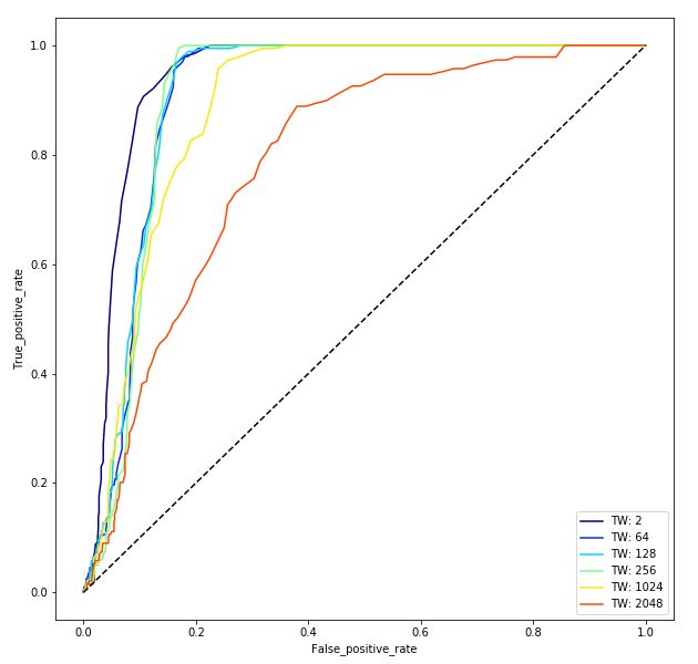
Robotics 2021, 10, 93                                                                                            2 of 11

                        of unusual behaviour or the degradation of performance, and report these findings to
                        the robot’s operator. Traditional CMS uses dedicated sensors to identify a fault in the
                        components; for example, a vibration sensor to identify the faults on a motor. In our work,
                        we made use of already existing data provided by the robot hardware to the operator and
                        to the control system. As will subsequently become clearer, an anomaly in these data is not
                        necessarily related to a fault in a robot component, but represents an unexpected event in
                        a wider sense. Differences in measurements of parameters such as position and velocity
                        can be noted by an expert operator without any additional system. Other measurements,
                        such as those of motor current, torque and temperature, are usually hidden to the operator
                        to avoid distractions. Moreover, the wealth of information available to operators during
                        a complex robot operation may be overwhelming. Variations in such measurements are
                        therefore impossible to be noted by an operator, even the most experienced one. From the
                        operator’s point of view, it is important to remain focused on performing the task and be
                        able to be informed with only the most relevant information in case a fault is developing.
                             In our work, we used Variational AutoEncoder to identify anomalies in our robotic
                        glovebox setup. This choice was motivated by the highly complex and structured nature of
                        the relationship between the measured signals and the robot’s health. Our main research
                        contribution is to propose a Monte Carlo-based technique to produce a statistic of expected
                        nominal behaviour and then use this to identify anomalies. To improve our results, we also
                        scored samples by using loss function scoring and we made use of the F1 score and ROC
                        score to tune the sensitivity to discriminate anomalies.
                             This paper is organized as follows. In the next section, we give a background on
                        anomaly detection and Variational AutoEncoder. In Section 3, we introduce a technique
                        to use the anomaly detection. In the subsequent section (Section 4), we introduce our
                        experimental setup. In Section 5, we report and discuss our results and in the final section,
                        we discuss our conclusions and outline future works.

                        2. Background
                        2.1. Anomaly Detection
                             Traditional fault detection techniques require detailed a priori knowledge of all the
                        possible faults that a robot may encounter. However, this is not always possible in chal-
                        lenging environments, as access to extensive characterisation is rarely feasible. This leads
                        to many faults occurring in a nuclear environment (for example) that are novel. However,
                        the existence of a fault can be inferred by a discrepancy with respect to the usual behaviour
                        in the robot’s data. Such discrepancy, or anomaly, in the data can represent different types
                        of data anomaly. In [1], the authors classify anomalies in the following three categories:
                        •    Point anomalies—where a single instance of the data is anomalous with respect to all
                             the rest of the data;
                        •    Contextual anomalies—where an instance of the data is anomalous with respect to the
                             specific context of the data; i.e., data that would be nominal in the context of a robot’s
                             linear motion would also be anomalous when the robot performs accelerating motion;
                        •    Collective anomalies—where a collection of the data is anomalous with respect to the
                             data set; e.g., data from the current sensor and thermometer are individually nominal,
                             but not both at the same time.

                        2.2. Variational AutoEncoder
                              In recent years, deep learning-based generative models have gained more and more
                        interest due to (and implying) some amazing improvements in the field. One such tech-
                        nique is the Variational AutoEncoder (VAE) [2]. In probability model terms, the VAE refers
                        to approximate inference in a latent Gaussian model where the approximate posterior
                        and model likelihood are parametrised by neural networks (the inference and generative
                        networks). In neural network language, a VAE consists of an encoder, a decoder, and a
                        loss function.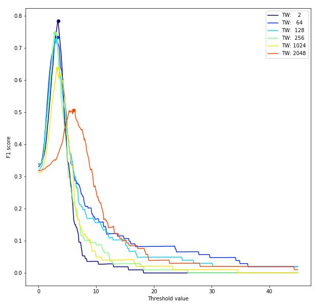
Robotics 2021, 10, 93                                                                                           3 of 11

                             The purpose of the encoder is to map the information included in the sample in a
                        reduced dimension space, called latent space. This space is meant to contain the main
                        characteristics of the samples. The decoder, on the other hand, maps a sample from its
                        latent space representation back to the original form. The peculiarity of the VAE is that
                        each dimension of the latent space consists of a Gaussian distribution, each of which is
                        characterised by a mean and a logarithmic variance value. This implies that, once a sample
                        is mapped in the latent space, it is possible to draw multiple times to obtain multiple
                        reconstructions of the original sample. In a VAE, the loss function is the sum of two parts:
                        reconstruction loss and latent loss. The reconstruction loss is a metric of the VAE ability to
                        reproduce the desired output; for example, such a loss can be the mean square error (MSE)
                        or the mean absolute percentage error (MAPE). The latent loss encourages the latent space
                        to have a form of Gaussian distribution; an example of latent loss is the KL divergence loss.
                             In recent years, VAE have been used for anomaly or fault detection in a wide range
                        of applications, from images to bank transactions. In [3], the authors combined VAE and
                        long short-term memory (LSTM) to detect anomalies in time series. In [4], the authors used
                        the VAE model to detect anomalies in videos. It is interesting to note that in the paper,
                        the latent space is modelled as a Gaussian mixture model (GMM) rather than a single
                        Gaussian distribution. In [5], the authors took advantage of multiple draws from the latent
                        space to map the reconstruction error, i.e., the difference between the input sample and its
                        reconstruction into Gaussian distribution. We do not think it is possible to apply the same
                        techniques to our data and therefore, as it will be clearer later in the paper, we adopted
                        a different method to identify anomalies. In [6], the authors discriminated anomalies by
                        clustering the latent space. Furthermore, in this case, we do not believe it is possible to
                        apply this technique to our data. In [7], the authors explored the use of conditional VAE for
                        anomaly detection in CERN LHC data.

                        3. VAE for Anomaly Recognition
                        3.1. Reconstruction
                             We trained the VAE to reproduce in the output the sample presented in the input. The
                        main idea was that the VAE would be able to reproduce a sample that already appeared
                        during training, while it would fail if a sample contained any kind of anomaly. A sample is
                        made by measurements collected from all the joints; in the case of an anomaly in a joint,
                        only some of the measurements will be affected.
                             Figure 1a,b illustrates a simplification of the reconstruction concept. In particular,
                        in normal conditions represented by Figure 1a, measurements collected from the robot are
                        collectively known, and therefore the VAE is able to reproduce all of them correctly. In the
                        case of measurements not already being collectively presented during training, as shown
                        in Figure 1b, the VAE will not be able to correctly reproduce them.
                             It is important to note that in Figure 1b, the anomalous measurement must not
                        necessarily be novel or contain values never seen before. The VAE will not be able to
                        reproduce all of these as long as they are not collectively the same.
                             One way of seeing this is that the state of the machine is then encoded in the latent
                        space. If the encoder encodes a region of the latent space that has not been trained,
                        the decoder will not be able to decode and thus coherently/correctly reproduce the values.
                        Following this analogy, using a VAE allows the system to account for sensor noise, and
                        the latent space can encode a covariance to the probability of values based on the region.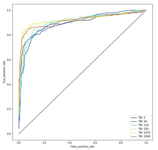
Robotics 2021, 10, 93                                                                                            4 of 11

                                                 (a) Normal condition behaviour.

                                               (b) Anomalous condition behaviour.
                        Figure 1. Simplified scheme of VAE reproducing data under normal conditions with anomalies.

                        3.2. Monte Carlo Reconstruction
                              One of the main advantages of using a VAE instead of an AutoEncoder is that having
                        a stochastic process as part of the latent space permits the generation of multiple recon-
                        structions of the predicted signal, starting from a single point in the latent space in a Monte
                        Carlo fashion. By separating the encoder and the decoder components of a trained VAE,
                        it is possible to use the encoder to obtain a latent space representation of a sample. From
                        here, it is then possible to sample the decoder multiple times, in a Monte Carlo fashion,
                        to collect a statistic of the expected reconstruction behaviour. The reconstruction of any
                        sample which is not compliant with this statistic can be interpreted as an anomaly. Another
                        advantage of using VAE is its robustness against noise. It is inevitable that there will be
                        a base level of noise in any sensor reading, as it is the case in entropy, so it will not be
                        possible for the decoder to reproduce this signal component exactly. However, the level of
                        noise compared to the signal could be encoded into the covariance of the VAE.
                              It is assumed that the noise can be approximated as a Gaussian in the latent space, as
                        the latent space would approximate the underlying parameters of the system. A Monte
                        Carlo ensemble decoded from the latent space can then approximate a nominal stochas-
                        tic distribution.
                              For example, it is possible to generate a zone around each signal showing nominal
                        behaviour. This zone can be calculated as the convex hull of all the expected reconstructed
                        measurements. Each signal reconstructed within this zone can be considered as nominal
                        behaviour, while the reconstructed sample outside of it can be considered an anomaly. A
                        Gaussian mixture model was investigated but deemed unnecessary. A schematic represen-
                        tation is shown in Algorithms 1 and 2. In particular, Algorithm 1 describes the process of
                        generating the zone in which a sample can be considered as having a nominal behaviour,
                        while Algorithm 2 describes the process of assessing the status of a sample.
Robotics 2021, 10, 93 5 of 11
Algorithm 1: Algorithm to construct nominal behaviour zone.
/* Retrieve encoder and decoder from a trained VAE */
encoder = trained_vae.get_encoder () ;
decoder = trained_vae.get_decoder () ;
/* Iterate over all the samples */
for sample s do
/* get latent space l (s) representation of the sample s */
l (s) = encoder (s) ;
for draw=1:1e6 do
/* get reconstructed sample s∗ from decoder */
s∗ = decoder (l (s)) ;
/* store all reconstructed sample s∗ */
set_o f _s∗ .append(s∗ )
end
/* define normal behaviour as envelope of all reconstructed
samples s∗ */
for each signal do
signal_normal_behaviour (s) = envelope(set_o f _s∗ , signal )
end
end
Algorithm 2: Algorithm to assess the status of a sample.
/* Iterate over all the samples */
for sample s do
/* get reconstructed sample s∗ from vae */
s∗ = vae(s) ;
/* assess against calculated nominal behaviour zone */
for each signal do
if s∗ ∈ signal_normal_behaviour (s) then
s_is_anomaly = False
else
s_is_anomaly = True
end
end
end
4. Experimental Setup
4.1. Glovebox Use-Case
The setup consists of two Kinova Gen 3, with seven degrees of freedom [8] and two
robotic arms, installed in the glovebox demonstrator [9]. The two robotic arms are identical,
but the end effectors attached to them considerably differ in terms of dimensions and
weights. The experiment will perform a series of CMS dedicated moves that are executed at
the beginning and at the end of operations. There are many advantages of using dedicated
moves, however, the main one is that they provide a solid and reliable base of data not
affected by any external factor, such as human error. Moreover, in a robotic glovebox
context and from the operational point of view, it is convenient to have “warm-up” and
“cool-down” phases at the beginning and at the end of operations, during which one can
ensure that the system is, respectively, ready to operate or has not been damaged during
the operations.
The glovebox system is controlled using the ROS framework [10,11]. The Kinova
ROS package provides a large amount of real-time data sampled at 1 KHz for each joint.
In particular, in our work, we use the joint position, joint velocity, motor current and motor
torque of each joint.Robotics 2021, 10, 93 6 of 11
It is very important to note that the measurements in use are very different from each
other and their range of extension is very diverse. This makes it very difficult to scale them
to a common range, i.e., between 0.0 and 1.0. Scaling each individual measurement with a
common scaling factor would have made features disappear; on the other hand, scaling
them with a measurement’s specific factor would have modified the relationship between
measurements—unless all data were scaled equally, which would potentially suppress
some values.
Not having all the input normalised between 0.0 and 1.0 creates a constraint in
the definition of the reconstruction loss. In fact, the same mean square error in two
different measurements can have different effects. For this reason, this work evaluates
the reconstruction error using the mean absolute percentage error (MAPE). Using MAPE
reconstruction loss, the same error in two different measurements is considered differently
according to the measurement magnitude.
To be able to capture the dynamic behaviour of the system, we chose to consider,
as a single sample, the data collected during a configurable time window. A sample is
therefore a matrix where each row represents a measurement and the columns represent
the acquisition times. In Figure 2, an example of the data coming from joint 3 sectioned in
the time window is presented.
Joint: 3 Position Joint: 3 Velocity
1.0
0.8 1.4
0.6
1.2
Velocity [rad/s]
0.4
Position [rad]
0.2 1.0
0.0
0.8
0.2
0.4 0.6
0.6
0 2000 4000 6000 8000 10,000 12,000 14,000 0 2000 4000 6000 8000 10,000 12,000 14,000
Time [sample] Time [sample]
2.75
Joint: 3 Current_motor Joint: 3 Torque
10
2.50
2.25 5
2.00
Torque [Nm]
Current [A]
1.75 0
1.50
1.25 5
1.00
10
0.75
0 2000 4000 6000 8000 10,000 12,000 14,000 0 2000 4000 6000 8000 10,000 12,000 14,000
Time [sample] Time [sample]
Figure 2. An example of time-windowed data sampled from a single joint for one glovebox robot.
It is important to note that this choice does not affect the capability of the system to
identify anomalies while working online in any way, as the current sample at time tnow
should be the set of data collected during the time window [tnow − twindow , tnow ). It is also
important to note that the longer the time window, the highest the amount of information
each sample contains is. On the other hand, using a long time window, the system becomes
less sensitive to short time perturbations. As will be explained later, the length of the time
window changes the behaviour of the system in identifying different types of faults.Robotics 2021, 10, 93 7 of 11
4.2. Implementation
Our VAE layout consists of a fully connected multiple-layer neural network. Through
testing, an optimal number of layers and their sizes were determined. Good results in
reproducing the input samples were obtained with the encoder’s layers dimensioned
512, 256, 128, 64, 32 and with a latent space with a dimension of 6. As the sample’s values
are not bonded between 0.0 and 1.0, a Leaky ReLu activation function was used. The
decoder was implemented in a symmetric way. For operational reasons, the VAE was
trained using data coming from only one of the two robots installed in the glovebox, from
now on the training robot. Data collected from the other robot, now referred to as the
testing robot, were used for comparison purposes.
In Figure 3, it is reported that data were reconstructed by the trained VAE. In particular,
reconstructed measurements of Joint 3 using data collected from the training robot are
reported in the figure, but not those used during VAE training. Black lines represent
original measurements, while the red lines represent the reconstructed measurements. To
increase the readability of the figure, the reconstructed data were reported only during
certain time windows.
Joint: 3 Position Joint: 3 Velocity
1.0
0.8 1.4
0.6
1.2
Velocity [rad/s]
0.4
Position [rad]
0.2 1.0
0.0
0.8
0.2
0.4 0.6
0.6
0 2000 4000 6000 8000 10,000 12,000 14,000 0 2000 4000 6000 8000 10,000 12,000 14,000
Time [sample] Time [sample]
Joint: 3 Current_motor Joint: 3 Torque
10
2.5
5
2.0
Torque [Nm]
Current [A]
0
1.5
5
1.0
10
0 2000 4000 6000 8000 10,000 12,000 14,000 0 2000 4000 6000 8000 10,000 12,000 14,000
Time [sample] Time [sample]
Figure 3. Example of data reconstructed by VAE. Original measurements not used during training are reported in black.
Different samples of output reproduced by the trained VAE are reported in red.
In Figure 4, we report the mean value of each latent space dimension over time.
Red lines represent results obtained from the training data, while blue lines represent the
results obtained from the testing robot data set.Robotics 2021, 10, 93 8 of 11
Latent space # 1 Latent space # 2
1
2
Mean value
Mean value
0
1 0
2
2
0 2000 4000 6000 8000 10,000 12,000 0 2000 4000 6000 8000 10,000 12,000
Time [sample] Time [sample]
Latent space # 3 Latent space # 4
2 2
Mean value
Mean value
1
0 0
1
2
2
0 2000 4000 6000 8000 10,000 12,000 0 2000 4000 6000 8000 10,000 12,000
Time [sample] Time [sample]
Latent space # 5 Latent space # 6
2
0
Mean value
Mean value
1
1
0 Training
Testing
1 2
0 2000 4000 6000 8000 10,000 12,000 0 2000 4000 6000 8000 10,000 12,000
Time [sample] Time [sample]
Figure 4. Example of data represented in latent space. Red lines represent results obtained from training data, while blue
lines represent results obtained from testing data.
5. Results
We used the Monte Carlo technique explained in Section 3.2 to generate a zone in
which we expected a signal with nominal behaviour.
In Figure 5a, the calculated zone in which the motor current of joint 3 is expected to
be reconstructed is shown in red, while the black line represents the actual measure. As
can be noted, the zone of expected nominal behaviour is very narrow.
In Figure 5b, multiple draws of samples collected from the testing robot (in blue) are
compared to the expected behaviour zone (in red). Data from the testing robot are clearly
different from the nominal behaviour and are definitively outside the zone of expected
behaviour. This is because the two robots are equipped with two different end effectors.
Joint: 3 Current_motor Joint: 3 Current_motor
2.75 Measurement
Measurement
Normal behaviour zone Normal behaviour zone
2.50 2.5
2.25
2.0
2.00
Current [A]
Current [A]
1.75
1.5
1.50
1.25
1.0
1.00
0.75
0.5
0 2000 4000 6000 8000 10,000 12,000 0 2000 4000 6000 8000 10,000 12,000
Time [sample] Time [sample]
(a) Training (b) Testing
Figure 5. Example of calculated nominal behaviour zone and its comparison with multiple reconstructions in the case of the
training and testing robot data.Robotics 2021, 10, 93 9 of 11
To improve the identification of anomalies, we opted to use the VAE loss function to
score a sample. We only focused on the training robot because the data coming from the
testing robot were already proven to be anomalous. As we did not experience any anomaly
with the training robot over time, we modified our data to generate simulated anomalies.
In particular, we modified our data in two different ways:
(a) Variation perturbation—a variation of 20% in some of a joint’s measurements;
(b) Swap perturbation—a swap between two time windows of some of the
joint’s measurements.
The first type of data perturbation was intended to reproduce a “point anomaly”,
where the perturbed data are anomalous with respect to all the rest of the data. In this sense,
we can imagine this anomaly as the data that assume values never seen before during the
training.
The second type of data perturbation was intended to reproduce a “contextual
anomaly”, where the perturbed data are anomalous in its context. In this sense, we
can imagine this anomaly as data that are not new, but anomalous because they are in the
wrong context.
We considered an anomaly as a sample for which the loss score is higher than a
predefined threshold. We calculated this threshold as the value that provides the maximum
F1 score. It is important to note that this is possible because we generated simulated faults,
and therefore, we obtained ground truth information on the data.
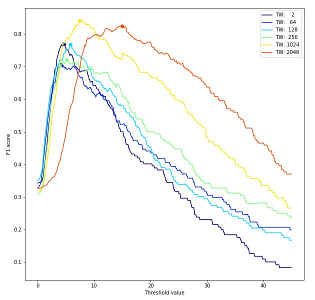
In Figure 6a,b, different values of the F1 score and ROC score are reported for different
values of the time windows in the case that the data are modified using a “variation
perturbation”.
Our results show that for this type of anomaly, the best F1 score is approximately 0.80,
and it is obtained with a time window of 2 samples (dark blue line). Small time windows
(2, 64, 128, 256) do have similar good performances, while longer time windows (1024 and
2048) have the worst performances. These results were also confirmed by the ROC score,
in which small time windows’ curves are closer to the top left corner. Intuitively, this was
equivalent to saying that as point anomalies are data that have never been seen before, they
are easier to recognise using short time windows.
(a) F1 scores (b) ROC scores
Figure 6. Trends of F1 score (a) and ROC score (b) curves for different values of time windows in the case of simulated
variation perturbation anomalies.Robotics 2021, 10, 93 10 of 11
Similarly, in Figure 7a,b, different values of the F1 score and ROC score are reported
for different values of the time windows in the case that data are modified using a “swap
perturbation”.
Our results show that for this type of anomaly, the best F1 score is approximately 0.85,
and it was obtained with a time window of 1024 (yellow line), which corresponds to ap-
proximately 2 s. Furthermore, in this case, it is possible to observe how long time windows
and short time windows perform in opposite ways. Intuitively, long time windows perform
better with the “swap perturbation” anomaly because the data are not novel in value in
this context, therefore the system needs more information to identify the anomalies.
Overall, these results show that the VAE provides very good accuracy in both types of
simulated anomalies.
(a) F1 scores (b) ROC scores
Figure 7. Trends of F1 score (a) and ROC score (b) curves for different values of time windows in the case of simulated
swap perturbation anomalies.
6. Discussion and Conclusions
In this paper, we investigated the use of VAE in identifying anomalous data collected
from our robotic glovebox setup. We defined a Monte Carlo-based technique to produce a
statistic of expected nominal behaviour results. We applied this technique to data collected
from two identical robots equipped with different end effectors. To improve our results,
we used a loss function score against simulated anomalies in the data. We proved that both
techniques can be used in the detection of anomalies in the data.
The stochastic process in the latent space allowed us to encode a sample into a latent
space and then draw from it multiple times, to obtain a statistic of the VAE ability to
reconstruct that sample. In contrast to [5], we decided to not assume that the reconstruction
error was Gaussian. Instead, we decided to use these statistics differently. Unfortunately,
the zone we obtained was too narrow to be practically useful. However, this may not be
true for less stable and more fault-prone systems.
As an alternative, we opted to use the VAE score to assess whether the sample was an
anomaly. To calculate the threshold to discriminate normal from anomalous behaviour, we
made use of F1 and ROC scores. Interestingly, the length of the time window influenced
the ability to identify different types of simulated anomalies. In particular, in simulated
context anomalies obtained by swapping values of different instants in time for some
measurements, long time windows performed better. This was expected as in this type of
anomaly, values were presented during training, but not collectively at the same time. ThisRobotics 2021, 10, 93 11 of 11
required more information to be available in the sample. On the other hand, in simulated
point anomalies, obtained by increasing the values of some measurements by 20%, the VAE
did not need much information to identify values which had never been presented before.
In this case, short time windows performed better.
One of the weaknesses of this study is the lack of any real anomaly data vs. actual
anomaly data. During our time with the Kinovas, we only witnessed one anomaly in 100 s
of hours of operations, which was identified by the proposed system. For future studies,
we propose that a more anomaly-prone system be used, rather than an industrial robot,
which are known for their robustness.
In future works, we will further investigate the possibility of using statistics from
multiple reconstructions of the same sample to identify anomalies or using a standard
auto-encoder to simplify the process.
Author Contributions: Conceptualization, L.P., G.B. and R.S.; methodology, L.P., G.B. and R.S.;
software, L.P.; validation, L.P. and G.B.; formal analysis, L.P., G.B. and R.S.; investigation, L.P.
and G.B.; resources, G.B. and R.S.; data curation, L.P.; writing—original draft preparation, L.P.;
writing—review and editing, L.P., G.B. and R.S.; visualization, L.P.; supervision, G.B. and R.S.; project
administration, G.B. and R.S.; funding acquisition, G.B. and R.S. All authors have read and agreed to
the published version of the manuscript.
Funding: This project was supported by the RAIN Hub, which was funded by the Industrial Strategy
Challenge Fund as part of the government’s modern industrial strategy. The fund was delivered by
the UK Research and Innovation and managed by EPSRC [EP/R026084/1].
Institutional Review Board Statement: Not Applicable.
Informed Consent Statement: Not Applicable.
Data Availability Statement: Not Applicable.
Conflicts of Interest: The authors declare no conflict of interest.
References
1. Chandola, V.; Banerjee, A.; Kumar, V. Anomaly detection: A survey. ACM Comput. Surv. 2009, 41, 15:1–15:58. [CrossRef]
2. Kingma, D.P.; Welling, M. Auto-encoding variational bayes. arXiv 2013, arXiv:1312.6114.
3. Lin, S.; Clark, R.; Birke, R.; Schönborn, S.; Trigoni, N.; Roberts, S. Anomaly Detection for Time Series Using VAE-LSTM Hybrid
Model. In Proceedings of the ICASSP 2020—2020 IEEE International Conference on Acoustics, Speech and Signal Processing
(ICASSP), Barcelona, Spain, 4–8 May 2020; pp. 4322–4326.
4. Fan, Y.; Wen, G.; Li, D.; Qiu, S.; Levine, M.D.; Xiao, F. Video anomaly detection and localization via gaussian mixture fully
convolutional variational autoencoder. Comput. Vis. Image Underst. 2020, 195, 102920. [CrossRef]
5. An, J.; Cho, S. Variational Autoencoder based Anomaly Detection using Reconstruction Probability. Spec. Lect. IE 2015, 2, 1–18.
6. Xu, H.; Feng, Y.; Chen, J.; Wang, Z.; Qiao, H.; Chen, W.; Zhao, N.; Li, Z.; Bu, J.; Li, Z.; et al. Unsupervised Anomaly Detection via
Variational Auto-Encoder for Seasonal KPIs in Web Applications. In Proceedings of the 2018 World Wide Web Conference on
World Wide Web—WWW ’18, Lyon, France, 23–25 April 2018; [CrossRef]
7. Pol, A.A.; Berger, V.; Cerminara, G.; Germain, C.; Pierini, M. Anomaly Detection with Conditional Variational Autoencoders.
CoRR. 2020. Available online: http://xxx.lanl.gov/abs/2010.05531 (accessed on 5 July 2021).
8. Kinova Gen 3 Product Description. Available online: https://www.kinovarobotics.com/en/products/gen3-robot (accessed on
21 May 2020).
9. Tokatli, O.; Das, P.; Nath, R.; Pangione, L.; Altobelli, A.; Burroughes, G.; Skilton, R. Robot Assisted Glovebox Teleoperation for
Nuclear Industry. Robotics 2021, 10, 85. [CrossRef]
10. Quigley, M.; Conley, K.; Gerkey, B.; Faust, J.; Foote, T.; Leibs, J.; Wheeler, R.; Ng, A.Y. ROS: An open-source Robot Operating
System. In Proceedings of the IEEE ICRA 2009, Kobe, Japan, 12–17 May 2009.
11. ROS: Robot Operating System. Available online: https://www.ros.org/ (accessed on 21 May 2020).You can also read