Vortex flow properties in simulations of solar plage region: Evidence for their role in chromospheric heating
←
→
Page content transcription
If your browser does not render page correctly, please read the page content below
A&A 645, A3 (2021)
https://doi.org/10.1051/0004-6361/202038965                                                                                                              Astronomy
c N. Yadav et al. 2020                                                                                                                                    &
                                                                                                                                                         Astrophysics

         Vortex flow properties in simulations of solar plage region:
              Evidence for their role in chromospheric heating
                                                  N. Yadav1,? , R. H. Cameron1 , and S. K. Solanki1,2

     1
         Max Planck Institute for Solar System Research, Justus-von-Liebig-Weg 3, 37077 Göttingen, Germany
         e-mail: nitnyadv@gmail.com, solanki@mps.mpg.de
     2
         School of Space Research, Kyung Hee University, Yongin, Gyeonggi 446-701, Republic of Korea

     Received 17 July 2020 / Accepted 27 October 2020

                                                                                    ABSTRACT

     Context. Vortex flows exist across a broad range of spatial and temporal scales in the solar atmosphere. Small-scale vortices are
     thought to play an important role in energy transport in the solar atmosphere. However, their physical properties remain poorly under-
     stood due to the limited spatial resolution of the observations.
     Aims. We explore and analyze the physical properties of small-scale vortices inside magnetic flux tubes using numerical simulations,
     and investigate whether they contribute to heating the chromosphere in a plage region.
     Methods. Using the three-dimensional radiative magnetohydrodynamic simulation code MURaM, we perform numerical simulations
     of a unipolar solar plage region. To detect and isolate vortices we use the swirling strength criterion and select the locations where
     the fluid is rotating with an angular velocity greater than a certain threshold. We concentrate on small-scale vortices as they are the
     strongest and carry most of the energy. We explore the spatial profiles of physical quantities such as density and horizontal velocity
     inside these vortices. Moreover, to learn their general characteristics, a statistical investigation is performed.
     Results. Magnetic flux tubes have a complex filamentary substructure harboring an abundance of small-scale vortices. At the inter-
     faces between vortices strong current sheets are formed that may dissipate and heat the solar chromosphere. Statistically, vortices have
     higher densities and higher temperatures than the average values at the same geometrical height in the chromosphere.
     Conclusions. We conclude that small-scale vortices are ubiquitous in solar plage regions; they are denser and hotter structures that
     contribute to chromospheric heating, possibly by dissipation of the current sheets formed at their interfaces.
     Key words. Sun: faculae, plages – Sun: chromosphere – methods: numerical – methods: statistical

1. Introduction                                                                                 lines. Analyzing G-band observations recorded with the Swedish
                                                                                                Solar Telescope (SST; Scharmer et al. 2003), Bonet et al. (2008)
Identifying the physical mechanisms responsible for the high                                    observed the swirling motions of bright points around intergran-
plasma temperatures in the solar atmosphere is a long-standing                                  ular points where several dark lanes converge. They interpreted
problem in solar physics. In recent years vortices have received                                these swirls as vortex flows driven by the granulation down-
increasing attention due to their importance in the heating                                     drafts. These vortices had sizes of ∼500 km and lifetimes on the
of the solar atmosphere (Moll et al. 2011; Shelyag et al. 2011;                                 order of 5 min. Large-scale (∼15−20 Mm) long-lasting (∼1−2 h)
Park et al. 2016; Murawski et al. 2018). Vortices are rotat-                                    vortex flows located at supergranular junctions were identified
ing plasma structures extending from the solar surface up to                                    by Attie et al. (2009) using time series observations by the Solar
coronal heights prevalent in active regions and in quiet-Sun                                    Optical Telescope/Filtergraph (SOT/FG; Ichimoto et al. 2008)
regions (Wedemeyer-Böhm et al. 2012; Tziotziou et al. 2018).                                    on board the Hinode satellite (Kosugi et al. 2007). Later, using
They couple different solar atmospheric layers and are thought                                  observations obtained with the Imaging Magnetograph eXperi-
to excite various magnetohydrodynamic (MHD) waves, includ-                                      ment (IMaX, Martínez Pillet et al. 2011) on board the balloon-
ing torsional Alfvén waves (Fedun et al. 2011; Shelyag et al.                                   borne observatory SUNRISE (Solanki et al. 2010; Barthol et al.
2013; Jess et al. 2015; Morton et al. 2013, 2015) that can heat                                 2011; Gandorfer et al. 2011; Berkefeld et al. 2011), Steiner et al.
the solar atmosphere (Shelyag et al. 2016; Liu et al. 2019a).                                   (2010) investigated the vortex motions in the intergranular lanes
They exist over a wide range of scales, with small-scale                                        and found the fine structure of numerous granules to consist of
short-lived vortices being the most abundant although not yet                                   moving lanes having a leading bright rim and a trailing dark
observed due to the limited spatial resolution of observations                                  edge. They compared the observational results with the numer-
(Kato & Wedemeyer 2017; Liu et al. 2019b; Giagkiozis et al.                                     ical simulations of solar surface convection, and interpreted
2018; Yadav et al. 2020).                                                                       these moving horizontal lanes as horizontal vortex tubes. Since
    Vortices have been observed in different atmospheric lay-                                   the average size of the observed vortex tubes (mean radius of
ers through various photospheric and chromospheric spectral                                     150 km) was close to the spatial resolution limits of the obser-
                                                                                                vations and the numerical simulations, they speculated that the
 ?                                                                                              occurrence of such features might extend to even smaller scales.
   Current address: Centre for Mathematical Plasma Astrophysics,
Department of Mathematics, KU Leuven, Celestijnenlaan 200B, 3001                                Bonet et al. (2010) used the same data set of observations, but
Leuven, Belgium.                                                                                a different analysis technique. They detected vertically oriented

                                                                                                                                                                            A3, page 1 of 9
               Open Access article, published by EDP Sciences, under the terms of the Creative Commons Attribution License (https://creativecommons.org/licenses/by/4.0),
                                which permits unrestricted use, distribution, and reproduction in any medium, provided the original work is properly cited.
                                                                  Open Access funding provided by Max Planck Society.
A&A 645, A3 (2021)

                                                                         tices. Using simulations, Kitiashvili et al. (2013) demonstrated
                                                                         that small-scale jet-like ejections in the chromosphere can be
                                                                         attributed to spontaneous upflows in vortex tubes. Moreover,
                                                                         there is observational evidence of the association of these rotat-
                                                                         ing structures with the heating of the chromospheric plasma
                                                                         (Park et al. 2016). Attie et al. (2016) analyzed the evolution of
                                                                         network flares and found them to occur at the junctions of net-
                                                                         work lanes, often in association with vortex flows. In a recent
                                                                         numerical study, Iijima & Yokoyama (2017) have investigated
                                                                         vortex flows as a driving mechanism for chromospheric jets and
Fig. 1. Sketch of the simulation box setup showing the location of the   spicules, and demonstrated that the Lorentz force of the twisted
mean solar surface at z = 0 (horizontal gray line).                      magnetic field lines plays an important role in the production
                                                                         of chromospheric jets. These studies indicate that even though
                                                                         they originate inside the downflowing intergranular lanes, vor-
vortices and attributed their origin to angular momentum con-            tices can support strong plasma upflows that may result in the
servation of the material sinking into the intergranular lanes.          formation of dynamic jet-like chromospheric features. In order
Requerey et al. (2018) explored the connection between a per-            to confirm a relationship between vortices and chromospheric
sistent photospheric vortex flow and the evolution of a mag-             heating, a statistical investigation is required.
netic element using observations acquired with Hinode. They                   The main objectives of this paper are to explore the physi-
found that magnetic flux concentrations occur preferably at vor-         cal properties of small-scale vortices and to investigate their role
tex sites, and the magnetic features often get weakened and frag-        in the heating of the solar chromosphere. In Sect. 2 we briefly
mented after the vortex disappears. Their study supports the idea        describe the details of the numerical simulations and the method-
that a magnetic flux tube becomes stable when surrounded by a            ology adopted for vortex identification. The results are presented
vortex flow (Schüssler 1984), and thus can support various MHD           and discussed in Sect. 3. The main points are summarized in
wave modes.                                                              Sect. 4, where our conclusions are drawn.
     Though the initial vortex studies were focused mostly
on photospheric vortices, these structures are not limited to
lower atmospheric layers. Vortex flows are also rather abun-             2. Methodology
dant in the chromosphere. Using observations obtained with
the CRisp Imaging Spectro-Polarimeter (CRISP) at the SST,                2.1. Numerical simulation: Computational setup
Wedemeyer-Böhm et al. (2012) analyzed chromospheric spec-
                                                                         We perform 3D radiation-MHD simulations using a new ver-
tral lines (e.g., Ca II 854.2 nm) and detected chromospheric
                                                                         sion of the MURaM code (Vögler et al. 2005; Rempel 2014,
swirls as dark and bright rotating patches. They estimated that
                                                                         2017) that can be extended to greater heights, thus reducing
there are as many as 11 000 chromospheric swirls (with a typi-
                                                                         the effect of the upper boundary. The simulation box covers
cal width of 1.5−4 Mm and lasting for 5−10 min) at any given
time, and they have associated photospheric bright points. They          12 Mm × 12 Mm × 4 Mm (with the third dimension referring to
interpreted these observations in terms of funnel-like magnetic          the direction perpendicular to the solar surface) that is resolved
field structures that have increasing cross-sectional area with          by 1200 × 1200 × 400 grid cells providing a spatial resolution
height and called them “magnetic tornadoes”. In addition to              of 10 km in all three directions. This high spatial resolution is
their direct detection in the photosphere and the chromosphere,          essential to detect the small-scale vortices and to study their fine
their imprints were also observed in the transition region and the       detail. In the vertical direction, it extends from 1.5 Mm beneath
lower corona through various ultraviolet (UV) and extreme ultra-         the mean solar surface to 2.5 Mm above it (see Fig. 1). We use
violet (EUV) channels of the Atmospheric Imaging Assembly                periodic boundary conditions in the horizontal direction, while
(AIA) on board the Solar Dynamics Observatory (SDO) space                the bottom boundary and the top boundary are kept open and
mission (Lemen et al. 2012).                                             closed, respectively, allowing the free in- and outflow of plasma
     Vortex flows have also been detected and analyzed                   from the bottom boundary while conserving the total mass in the
in three-dimensional (3D) radiation-MHD numerical simula-                computational box. The magnetic field is vertical at the top and
tions. A detailed investigation of vortices was performed by             bottom boundaries.
Shelyag et al. (2011) using magnetic and non-magnetic 3D                     We initialize the simulations by running a purely hydrody-
numerical simulations. Performing radiative diagnostics of the           namic case for almost 2 h of solar time, so that it reaches a
simulation data, they revealed the correspondence between the            statistically stationary state. Then we introduce a uniform ver-
rotation of magnetic bright points at the solar surface and              tical field of 200 G magnetic strength in a hydrodynamical snap-
small-scale swirls present in the upper photosphere (∼500 km             shot to simulate the conditions of a unipolar plage region, and
above the approximate visible solar surface level) of simulations.       we let the system evolve again for 1.2 h of solar time. In the
Kitiashvili et al. (2012) investigated the thermodynamic proper-         course of the simulations, magnetic field lines are advected by
ties of magnetized vortex tubes in quiet-Sun simulations and dis-        the plasma flows in the photosphere and strong magnetic ele-
cussed their importance in energy transport to the chromosphere.         ments of 1−2 kG are formed at the solar surface. We collect the
They found that vortex motions concentrate the magnetic fields           snapshots for 7 min at 10 s cadence for the vortex analysis.
in near-surface layers, which in turn stabilizes the vortex tubes,
reducing the influence of surrounding turbulent flows.                   2.2. Vortex identification
     Vortices are also related to dynamic jet-like features
observed in the chromosphere. Analyzing SST observa-                     There is no universally accepted definition for vortices in turbu-
tions, De Pontieu et al. (2012) reported spicules as supporting          lent fluids (Jeong & Hussain 1995) Though we have an intuitive
torsional Alfvén waves that can be excited by photospheric vor-          understanding of vortices as 3D objects, it is difficult to decide
A3, page 2 of 9
N. Yadav et al.: Small-scale vortices in the plage chromosphere

      (a) 12                                                  1.0         (b) 12                                                4.0
          10                                                                  10

                                                                                                                                          x10−7 ρ(g cm−3)
                                                              0.5                                                               3.5

                                                                     x102 Bz (G)
                  8                                                                8
        y (Mm)

                                                                       y (Mm)
                  6                                           0.0                  6                                            3.0
                  4                                                                4
                                                              -0.5                                                              2.5
                  2                                                                2
                  0                                           -1.0                 0                                            2.0
                      0   2   4 6 8              10 12                                 0   2     4 6 8             10 12
                               x (Mm)                                                             x (Mm)
       (c) 12                                                  6.6        (d) 12                                                6
           10                                                  6.4            10                                                4

                                                                                                                                     x105 vz (cm s−1)
                  8                                                                8                                            2
                                                                     x103 T(K)
         y (Mm)

                                                                      y (Mm)
                                                               6.2
                  6                                                                6                                            0
                                                               6.0
                  4                                                                4                                            −2
                  2                                            5.8                 2                                            −4
                  0                                            5.6                 0                                            −6
                      0   2    4 6 8              10 12                                0   2     4 6 8             10 12
                                x (Mm)                                                            x (Mm)
Fig. 2. Spatial maps of (a) vertical component of magnetic field (Bz ), (b) mass density (ρ), (c) temperature (T), and (d) vertical component of
velocity (vz ) at the τ = 1 layer, where τ is the continuum optical depth at 500 nm.

on where each ends. As there is no objective definition of a vor-          swirling time (τci ) by the relation λci = 2π/τci . The swirling time
tex, various vortex detection criteria are in use.                         signifies the rotation period of a vortex, whereas the swirling
     In the context of solar physics, the two most frequently              strength gives the angular velocity or angular frequency. The
used vortex detection criteria in simulations are enhanced vor-            eigenvector corresponding to the real eigenvalue at these loca-
ticity (Shelyag et al. 2013; Lemmerer et al. 2017) and enhanced            tions gives the direction vector of the vortex axis. To extract
swirling strength (Moll et al. 2011, 2012). Enhanced swirling              and isolate the vortices for further investigation, we select only
strength (Zhou et al. 1999) is considered to be a better detec-            those contiguous features that rotate significantly rapidly (i.e.,
tion method, as vorticity can be high even in non-rotating shear           with swirling times of less than 100 s) and have more than 200
flows. Kato & Wedemeyer (2017) compared these two vortex                   grid points in 3D space in each feature to avoid smaller transient
detection methods by applying them to the data obtained from               structures. The threshold in swirling time (or swirling strength)
3D numerical simulations and found that the enhanced swirling              is chosen by visual inspection of swirling strength maps at vari-
strength method is superior to the enhanced vorticity method in            ous heights such that the selected regions encompass the strongly
all aspects. Previously, Moll et al. (2011) successfully applied           rotating vortices.
the swirling strength criterion to identify small-scale vortices
in quiet-Sun simulations and found vortices with a spatial size
∼100 km in the near-surface layers of the convection zone and in
                                                                           3. Results
the photosphere. These results indicate that the swirling strength
criterion is the method of choice for our setup, which is similar          Figure 2 displays the maps of various physical quantities at
to that used in Moll et al. (2011), except that our simulation box         the corrugated τ = 1 layer (continuum formation height).
reaches much higher into the solar atmosphere.                             Panel a displays the vertical component of the magnetic field
     To identify vortices by the swirling strength criterion the           strength with values saturated at ±100 G. Small-scale mixed-
velocity gradient tensor, its three eigenvalues, and corresponding         polarity magnetic fields surrounding the strong magnetic field
three eigenvectors are calculated for all grid points using all three      concentrations are seen. Panel b shows the mass density (ρ);
components of velocity at each grid point. The grid points with            the mass density is higher in the intergranular lanes due to the
complex conjugate eigenvalues are essentially the vortex loca-             buildup of excess pressure there to stop the horizontal convec-
tions. The imaginary part of their complex conjugate eigenval-             tive flows. However, the strong magnetic field concentrations
ues represents the swirling strength (λci ), which is related to the       have low mass densities due to horizontal pressure balance. The
                                                                                                                                A3, page 3 of 9
A&A 645, A3 (2021)

          (a) 12                                                        3.5                        (b)
                                                                                                         0.4
                     10                                                 3.0
                                                                                                         0.2

                                                                              Intensity (x 1010)
                     8
                                                                        2.5
            y (Mm)

                     6                                                                                   0.0
                                                                        2.0
                     4                                                                               -0.2
                                                                        1.5
                     2
                                                                                                     -0.4
                     0                                                  1.0
                          0   2     4      6   8          10      12                                           -0.4   -0.2   0.0   0.2   0.4
                                        x (Mm)
Fig. 3. Bolometric intensity map: (a) over the whole simulation domain and (b) zoomed into a magnetic element.

Fig. 4. Three-dimensional visualization of vortices in a sub-domain of the simulation box (dimension: 12 Mm × 12 Mm × 1.4 Mm, with the mean
solar surface in the center). The corrugated τ = 1 layer (continuum formation height) is color-coded according to the vertical component of magnetic
field strength (see color bar on the left). The dark green structures are vortices identified via the swirling strength criterion.

temperature is displayed in panel c. Clearly, in the intergran-            magnetic region has been enlarged and is displayed in panel b.
ular lanes it is highly structured. The vertical component of              Ribbon- or flower-like intensity structures with bright edges can
velocity (vz ) is displayed in panel d. Convection is quenched             be seen in the intergranular lanes, caused by the complex interac-
by strong magnetic fields in magnetic concentrations, hence                tion of convection, magnetic fields, and radiation. Such intensity
we have almost negligible flows inside the strong magnetic                 profiles have been observed previously in a unipolar ephemeral
elements.                                                                  region (Narayan & Scharmer 2010).
    The map of bolometric intensity (i.e., intensity integrated                Figure 4 shows a sub-domain of the simulation box (dimen-
over all wavelengths) is displayed in panel a of Fig. 3. A small           sion: 12 Mm × 12 Mm × 1.4 Mm, with the mean solar surface

A3, page 4 of 9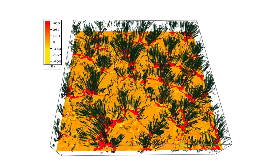
N. Yadav et al.: Small-scale vortices in the plage chromosphere

                12                                                               6

                10                                                               4

                8                                                                2
       y (Mm)

                                                                                     vz (km/s)
                6                                                                0

                                                                                                 2.5 Mm
                4                                                                -2

                2                                                                -4

                                                                                                             mM
                                                                                                          1.4
                0                                                                -6
                 0          2        4 6 8                     10 12                                              1.4 Mm
                                      x (Mm)
Fig. 5. Plasma flow velocity and magnetic field in vortices. Left: vertical component of flow velocity (vz ) at the τ = 1 layer with black contours of
Bz ranging from 400 G to 2500 G and a red box highlighting one magnetic element (right panel), where the image at the bottom now shows the
vertical component of the field, Bz , instead of vz in the left panel. Right: 3D view of a sub-domain covering the volume 1.4 Mm × 1.4 Mm × 2.5 Mm
corresponding to the red square in the left panel. Velocity streamlines and magnetic field lines are shown in sea green and deep purple, respectively,
at the selected vortex locations. A perpendicular cut at 1.5 Mm above the surface is indicated by the pink plane whose vortex properties will be
shown and discussed later in the paper.

in the center of the z-axis range). Only a restricted height range          these three vortices in this magnetic element are examined and
is displayed in this figure to clearly represent the foot points of         shown in Figs. 6 and 7. Though we present results for a single
vortex features, which become volume-filling in the upper lay-              magnetic element, several other magnetic elements are examined
ers. The vertical component of magnetic field strength at the               and are found to show qualitatively similar behavior.
τ = 1 layer is displayed by a color map (the color bar is saturated              Figure 6 displays the spatial profiles of various physical
at ±400 G for better visualization). The magnetic field strength            quantities in the selected magnetic element at the mean solar
in small magnetic elements typically lie in the range ∼1−2 kG               surface (left column) and at 1.5 Mm above the surface (right col-
at the solar surface and vortices originate inside these mag-               umn). Vortices are outlined in black. We note that we applied
netic concentrations. Vortices are selected using the enhanced              a swirling strength threshold to detect vortices and swirling
swirling strength criteria described in Sect. 2.2, and are shown            strength increases with height (see Fig. 7). Therefore, we missed
in dark green. Here, we take the swirling period threshold to               the comparatively smaller and slower rotating photospheric
be 100 s which corresponds to a swirling strength threshold of              counterparts of many chromospheric vortices. However, in the
0.0628 rad s−1 . Consequently, only those vortices are selected             photosphere many vortices have been detected in the surround-
that rotate with an angular velocity higher than this swirling              ings of the magnetic element where mixed-polarity magnetic
strength threshold.                                                         fields exist. As these mixed-polarity regions are highly turbu-
                                                                            lent and are strongly influenced by external flows, they undergo
                                                                            continuous flux cancellation and reconnection. Therefore, vor-
3.1. Individual vortices
                                                                            tices originating in these regions are extremely short-lived
Figure 5 displays the vertical component of flow velocity at the            (a few seconds) and do not extend higher up in the atmosphere.
τ = 1 layer (same as in Fig. 2) with overplotted contours of                In contrast, the vortices that originate inside the magnetic con-
the vertical component of magnetic field strength ranging from              centration extend up to the chromosphere following the mag-
400 G to 2500 G. To investigate the characteristics of the indi-            netic field lines and may transport energy into the chromosphere
vidual vortices in detail, an area with a horizontal extent of              (Yadav et al. 2020). Three squares are shown in each panel at
1.4 Mm × 1.4 Mm encompassing a magnetic element is selected                 the locations of the selected vortices. The areas of these squares
(marked by a red square in the figure). The 3D sub-domain of the            (i.e., cross-sectional areas of the vortices) grow from the photo-
simulation box corresponding to the red square is displayed on              sphere (left column) to the chromosphere (right column) due to
the right. This sub-domain extends 2.5 Mm in the vertical direc-            the expansion of the magnetic flux tube hosting the vortices with
tion above the mean solar surface. Though there are numerous                height. In addition, the locations of the vortices are not exactly
vortices present in this selected region, we have selected three            the same at the two heights because the cores of these vortices
vortices for visualization using VAPOR (Clyne & Rast 2005;                  are curved and obliquely directed.
Clyne et al. 2007). Velocity streamlines over these vortices are                 Row (a) of the figure displays the vertical component of the
displayed in seagreen, indicating fluid rotation. In contrast, the          magnetic vector. The magnetic field is concentrated in the photo-
magnetic field lines, displayed in deep purple, are aligned with            sphere, whereas in the chromosphere it is almost homogeneous
the axes of the vortex cores. The various physical properties of            (varying by less than 20% in the plotted region). Mass density

                                                                                                                                      A3, page 5 of 9
A&A 645, A3 (2021)
Bz (G) Bz (G) Swirling Strength (x10−2 rad/s) ρ (x10−7 g/cm3) Vh (km/s)
500 0 500 1000 1500250 262 275 288 300 0.0 1.5 3.0 4.5 6.0 0.6 0.8 1.0 1.2 1.4 1.6 0 1 2 3 4
(a)
700 60
40
20
350
y (km)
0
y (km)
−20
0 −40
−60
60
350
40
20
700
y (km)
0
x10 7 (g cm 3) x10 11 (g cm 3)
−20
0.00 1.25 2.50 3.75 5.00 0.0 0.5 1.0 1.5 2.0
(b) −40
700 −60
60
350 40
20
y (km)
y (km)
0
0
−20
−40
350 −60
−60 −40 −20 0 20 40 60 −60 −40 −20 0 20 40 60 −60 −40 −20 0 20 40 60
x (km) x (km) x (km)
700
x 106 Jz (biot cm-2) x 104 Jz (biot cm-2) Swirling Strength (x10−2 rad/s) ρ (x10−12 g/cm3) Vh (km/s)
0.00 3.75 7.50 11.25 15.00 0 2 4 6 8 10 0 4 8 12 16
-1.0 -0.5 0.0 0.5 1.0 -2 -1 0 1 2
(c) 100
700
50
y (km)
350
0
y (km)
−50
0
−100
100
-350
50
y (km)
-700
0
T (K) T (K)
5000 5450 5900 6350 6800 4400 4850 5300 5750 6200 −50
(d)
700 −100
100
350 50
y (km)
y (km)
0
0
−50
-350 −100
−100 −50 0 50 100 −100 −50 0 50 100 -100 -50 0 50 100
x (km) x (km) x (km)
-700
-700 -350 0 350 700 -700 -350 0 350 700 Fig. 7. Left to right: profiles of swirling strength, mass density, and hor-
x(km) x (km)
izontal velocity for three vortices different rows with border colors cor-
Fig. 6. Maps of (a) vertical component of the magnetic vector (Bz ), (b) responding to those of the squares outlining the vortices in Fig. 6 on the
mass density (ρ), (c) vertical component of current (Jz ), and (d) tem- solar surface (rows 1–3) and at 1.5 Mm above the surface (rows 4–6).
perature (T) at the mean surface (left column) and in the chromosphere The overplotted arrows represent the horizontal velocity. The longest
(right column). Three colored squares mark the locations of the selected arrow corresponds to 4 km s−1 and 16 km s−1 in the photosphere and the
vortices shown in Fig. 5. chromosphere, respectively.
maps are displayed in row (b). Vortices originating in the strong have lower temperatures at a given geometric height1 as they are
magnetic field concentrations have a lower density in the near in the strong magnetic concentration, while in the chromosphere
surface layers because strong magnetic regions are evacuated they often have high temperatures and heating appears to be local
due to pressure balance. In the chromosphere, however, they and co-located with current sheets in row (c).
capture the neighboring plasma and we see high-density intru- To analyze the vortex characteristics in detail the three vor-
sions, particularly in the lower half of the plotted panel (see, tices shown in Fig. 5 are investigated individually. The maps of
e.g., the green square). In row (c) of the figure, maps of the verti- various physical quantities over vortices with overplotted veloc-
cal component of the current are displayed. In the chromosphere ity vectors are shown in Fig. 7. Here the top three rows corre-
currents have a tendency to be stronger where there are more spond to the mean solar surface, while the bottom three rows
vortices, and they are primarily generated at the boundaries of correspond to the chromosphere. The spatial extents of vortices
the vortices due to shearing of the magnetic fields. In addition,
the regions without vortices have negligible currents. Tempera- 1
At equal optical depth, however, these locations are often hotter (e.g.,
ture maps are displayed in row (d). In the photosphere vortices Solanki 1993).
A3, page 6 of 9
N. Yadav et al.: Small-scale vortices in the plage chromosphere
(a) 0.20 (d) 1.6
Average normalized mass density
Fractional area coverage
0.15 1.3
0.10 1.0
0.05 0.7
0.00 0.4
(b) 450 Average over vortices (e) 6500 Average over vortices
Horizontal mean Horizontal mean
Average magnetic field (G)
375 5875
Temperature (K)
300 5250
225 4625
150 4000
(c) 2.0 (f) 3.5
Average normalized current (|Jz|)
3.0
1.5
2.5
Heating Fraction
2.0
1.0
1.5
1.0
0.5
0.5
0.0 0.0
0.5 1.0 1.5 2.0 2.5 0.5 1.0 1.5 2.0 2.5
z (Mm) z (Mm)
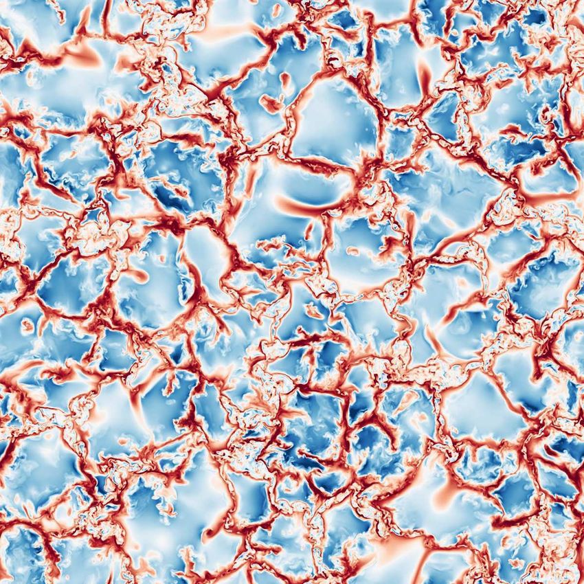
Fig. 8. Dependence of vortex properties on height. (a) Area fraction (fill factor) covered by vortices; (b) horizontally averaged magnetic field
strength in vortices (solid) and over the whole domain (dashed); (c) horizontally averaged unsigned vertical component of current in vortices
(normalized to the density averaged over the whole domain); (d) horizontally averaged mass density in vortices (similarly normalized); (e) hor-
izontally averaged temperature in vortices (solid curve) and over the entire domain (dashed curve); and (f ) horizontally averaged total heating
(viscous+resistive) in vortices (normalized to the total heating averaged over the whole domain). The region near the top boundary is shaded gray
and may be affected by the imposed top boundary conditions and should be ignored.
are different at these two layers as the vortices expand with mosphere, the plasma rotates faster near the edges than at the
height and have a larger cross-sectional area in the chromo- center in terms of absolute speed. However, the angular velocity
sphere than in the photosphere. The color of the borders of dif- is greater closer to the center.
ferent panels refers to the color of the squares in Fig. 6. The
first column displays the swirling strength profiles. Swirling 3.2. Statistical properties of vortices
strength increases radially towards the center of each vortex
which implies that the angular velocity increases, indicating that In a recent study Yadav et al. (2020) demonstrate that vortices
the vortices do not rotate as a rigid body. Furthermore, since exist over a range of spatial scales and smaller vortices are the
the average mass density is lower in the chromosphere than in dominant carriers of energy. Therefore, in the present paper
the photosphere, vortices rotate faster and have higher values of we concentrate on investigating the properties of small-scale
swirling strength (angular velocity) in the chromosphere in com- vortices. To study their general characteristics, a statistical inves-
parison to the photosphere. In addition, their shape may evolve tigation is performed by taking the temporal average for 42 snap-
quickly from the photosphere to the chromosphere. One of the shots covering a seven-minute time sequence at 10 s cadence.
three vortices remains roughly circular in shape over the whole The vortices that we are investigating are small-scale (spatial
height range, whereas the other two are quite elongated in the size of ∼50−100 km near the solar surface and ∼100−200 km in
chromosphere. The second column displays the maps of mass the chromosphere) and short-lived (lifetime ∼20−120 s). They
density. Vortices that reach up to the chromosphere are located are abundant throughout the simulation domain, therefore the
in regions of lower mass density (inside strong magnetic con- time sequence of seven minutes is sufficient for their statistical
centrations) at the mean solar surface; they nonetheless capture analysis. We display the dependence of vortex properties with
and trap plasma from the surroundings. A similar pattern is visi- height in Fig. 8. We note that the height scale starts at 0.5 Mm
ble in the three bottom rows corresponding to the chromosphere. above the average solar surface (i.e., roughly at the base of the
The maps of the horizontal flow velocity are displayed in the chromosphere). Panel a displays the filling factor of vortices (i.e.,
third column of the figure. At the solar surface and in the chro- the fractional area covered by vortices as a function of height).
A3, page 7 of 9
A&A 645, A3 (2021)

                                                                             geometrical height. The average temperature over vortices is
                                                                             always higher than the horizontally averaged temperature at the
                                                                             same geometrical height indicating their importance in the heat-
                                                                             ing of the chromosphere. We note that in lower layers (around
                                                                             z = 0) the temperature in vortices is lower than the aver-
                                                                             age as they are located in magnetic elements that are cooler at
                                                                             equal geometrical height. Panel f displays the total heating (vis-
                                                                             cous+resistive) over vortices relative to the horizontally aver-
                                                                             aged heating. Excessive heating over the vortices indicates their
                                                                             energetic importance, especially in the upper chromosphere. The
                                                                             results obtained in the uppermost layers (gray shaded region in
                                                                             all panels) should be ignored as they are affected by the closed
                                                                             top boundary condition, and therefore can be of non-physical
                                                                             origin.
                                                                                 In view of the results obtained we suggest the following for-
                                                                             mation mechanism for the small-scale vortices and display it
                                                                             in a simplified cartoon in Fig. 9. Vortices are formed at var-
                                                                             ious scales starting from the sizes of the intergranular lanes,
                                                                             possibly due to the angular momentum conservation of down-
                                                                             flowing plasma. Because of the turbulent nature of the plasma,
                                                                             vorticity cascades from the injection scale to the smaller scales.
                                                                             The smallest scales that can be resolved in our simulations
                                                                             correspond to a multiple of the grid resolution. In the upper
                                                                             convection zone and near-surface layers, where the ratio of ther-
                                                                             mal gas pressure to magnetic pressure (i.e., plasma-β) is high,
                                                                             the gas dynamics dominates over magnetic fields and magnetic
                                                                             field lines are frozen into the plasma. Vortical flows in this layer
                                                                             create a twist in the magnetic field. This twist in the magnetic
                                                                             flux tubes then propagates to higher atmospheric layers in the
Fig. 9. Simplified cartoon showing how turbulent motions drive vortices      form of a torsional Alfvén wave. In the upper layers, plasma-
on different spatial scales. The lines with arrow heads represent the sur-   β is low and the plasma dynamics is dominated by magnetic
face flows, being convective motions in the granules and small-scale         fields. Here, the twisted magnetic flux tubes make the surround-
turbulent motions in the intergranular lanes. These turbulent motions        ing plasma co-rotate forming a chromospheric counterpart of the
cover a range of scales and couple to the magnetic field (dashed curves)     photospheric vortices. Because of the inherent turbulence, larger
producing vortices at various scales from the whole flux tube (upper         vortex flows cascade down to the smallest sizes determined by
panel) down to the resolution limit of the simulation (lower panel).         the grid resolution and numerical diffusivity. Using vortex detec-
                                                                             tion methods based on velocity gradients, we select the smallest
                                                                             vortices present in the system. Vortices originate inside the mag-
In the lower chromospheric layers, the area coverage increases               netic elements and are aligned along the magnetic field lines
with height because of the magnetic field expansion; however, in             (as shown in Figs. 4 and 5). These vortices do not appear in
the upper layers magnetic field is nearly homogeneous (shown                 funnel-like shapes, as observed in quiet-Sun vortex observations
in panel b) and hence the filling factor of vortices does not                (Wedemeyer-Böhm et al. 2012; Park et al. 2016; Tziotziou et al.
increase much. Panel b displays the height variation of the aver-            2018), because vortices follow the magnetic field lines and the
age magnetic field strength over vortices (solid) and horizontal             magnetic flux tubes in active regions do not expand as much as in
mean (dashed). Up to a height of ∼1 Mm, vortices have higher                 the quiet-Sun regions, at least above the temperature minimum
averaged magnetic field strengths as they originate inside the               layer where the magnetic elements merge (Pneuman et al. 1986).
magnetic concentrations. However, in the higher layers, the field
strength is nearly homogeneous and the average magnetic field                4. Conclusions
over vortices is nearly same as the overall horizontal mean. Panel
c displays the vertical component of current (unsigned) averaged             Vorticies are ubiquitous in the solar atmosphere and it has
over vortices relative to the horizontal mean at the same geomet-            been suggested that they play an important role in the heat-
rical height confirming the association of small-scale vortices              ing of the solar atmosphere (Wedemeyer-Böhm et al. 2012;
with strong currents in the chromosphere, which we reported in               Tziotziou et al. 2018; Liu et al. 2019b). However, even with the
Sect. 3.1. The mass density averaged over the vortices at a given            highest resolution observations available, the internal structure
height relative to the density averaged over the entire horizon-             of the vortex tubes is not yet resolved. Moreover, small-scale
tal domain at the same geometrical height is displayed in panel              vortices are more abundant and are shown to contribute more
d. Up to a height of ∼1 Mm vortices have a lower mass density                energy flux in the solar atmosphere than comparatively larger
than the average mass density at the same geometrical height.                vortex flows (Yadav et al. 2020). Thus, it is of considerable
This is due to their occurrence in strong magnetic regions that              relevance to investigate their physical properties using high-
are evacuated. Above ∼1 Mm vortices have ∼50% higher den-                    resolution numerical simulations. With this aim, a 3D radiation-
sity than the average at that height as vortices trap the plasma             MHD simulation of a plage region was carried out. Using
in the chromosphere. Panel e shows the comparison of the aver-               the swirling strength criterion, vortices were detected and iso-
age temperature over vortices (solid curve) with the temperature             lated. We report the occurrence of very small-scale vortices in
averaged over the whole horizontal plane (dashed curve) at each              a unipolar plage region. With diameters of ∼50−100 km in the
A3, page 8 of 9
N. Yadav et al.: Small-scale vortices in the plage chromosphere

photosphere and ∼100−200 km in the chromosphere, these are                            Barthol, P., Gandorfer, A., Solanki, S. K., et al. 2011, Sol. Phys., 268, 1
the smallest vortices that can be resolved in our simulations. Due                    Berkefeld, T., Schmidt, W., Soltau, D., et al. 2011, Sol. Phys., 268, 103
to a lack of spatial resolution, such small-scale vortices have not                   Bonet, J. A., Márquez, I., Sánchez Almeida, J., Cabello, I., & Domingo, V. 2008,
                                                                                          ApJ, 687, L131
been detected in observations yet.                                                    Bonet, J. A., Márquez, I., Sánchez Almeida, J., et al. 2010, ApJ, 723, L139
    Vortices have a lower mass density than the mean density                          Brandenburg, A. 2014, ApJ, 791, 12
both in the photosphere and in the lower chromosphere; this is                        Brandenburg, A., & Rempel, M. 2019, ApJ, 879, 57
in agreement with the previous simulations that were limited to                       Clyne, J., & Rast, M. 2005, Proc. SPIE-IS&T Electron. Imaging, 5669, 284
                                                                                      Clyne, J., Mininni, P., Norton, A., & Rast, M. 2007, New J. Phys., 9, 301
the photosphere and lower solar chromosphere (Moll et al. 2011;                       De Pontieu, B., Carlsson, M., Rouppe van der Voort, L. H. M., et al. 2012, ApJ,
Kitiashvili et al. 2013). However, in the higher atmospheric lay-                         752, L12
ers, the vortices are denser than in the surroundings. This find-                     Fedun, V., Shelyag, S., Verth, G., Mathioudakis, M., & Erdélyi, R. 2011, Annal.
ing conforms with the fact that vortices are mostly observed                              Geophys., 29, 1029
as absorbing (dark) intensity structures when observed in chro-                       Gandorfer, A., Grauf, B., Barthol, P., et al. 2011, Sol. Phys., 268, 35
                                                                                      Giagkiozis, I., Fedun, V., Scullion, E., Jess, D. B., & Verth, G. 2018, ApJ, 869,
mospheric radiation (Wedemeyer-Böhm et al. 2012; Park et al.                              169
2016; Tziotziou et al. 2018).                                                         Ichimoto, K., Lites, B., Elmore, D., et al. 2008, Sol. Phys., 249, 233
    In chromospheric layers the temperature averaged over vor-                        Iijima, H., & Yokoyama, T. 2017, ApJ, 848, 38
tices is higher than the temperature averaged over the whole                          Jeong, J., & Hussain, F. 1995, J. Fluid Mech., 285, 69
                                                                                      Jess, D. B., Morton, R. J., Verth, G., et al. 2015, Space Sci. Rev., 190, 103
horizontal domain in the chromosphere (Fig. 8). Previously,                           Kato, Y., & Wedemeyer, S. 2017, A&A, 601, A135
Moll et al. (2012) had also found an association of stronger vor-                     Kitiashvili, I. N., Kosovichev, A. G., Mansour, N. N., & Wray, A. A. 2012, ApJ,
tices with increased temperatures (in simulations limited up to                           751, L21
800 km above the mean solar surface). Using simultaneous obser-                       Kitiashvili, I. N., Kosovichev, A. G., Lele, S. K., Mansour, N. N., & Wray, A. A.
vations from SST/CRISP and IRIS, Park et al. (2016) have also                             2013, ApJ, 770, 37
shown small-scale quiet-Sun vortices to have higher temperatures                      Kosugi, T., Matsuzaki, K., Sakao, T., et al. 2007, Sol. Phys., 243, 3
                                                                                      Kuridze, D., Zaqarashvili, T. V., Henriques, V., et al. 2016, ApJ, 830, 133
than the surroundings in the upper chromosphere. A particularly                       Lemen, J. R., Title, A. M., Akin, D. J., et al. 2012, Sol. Phys., 275, 17
important result of our present analysis is that we found thin and                    Lemmerer, B., Hanslmeier, A., Muthsam, H., & Piantschitsch, I. 2017, A&A,
strong current sheets that develop at their interface. There seems                        598, A126
to be a correspondence between high values of current densi-                          Liu, J., Nelson, C. J., Snow, B., Wang, Y., & Erdélyi, R. 2019a, Nat. Commun.,
ties and the vortex locations. Hence we conjecture that heating                           10, 3504
                                                                                      Liu, J., Nelson, C. J., & Erdélyi, R. 2019b, ApJ, 872, 22
at the vortex sites could be due to current dissipation in addition                   Martínez Pillet, V., del Toro Iniesta, J. C., Álvarez-Herrero, A., et al. 2011, Sol.
to viscous dissipation. Nonetheless, the ratio of viscous and resis-                      Phys., 268, 57
tive heating will depend on the magnetic Prandtl number, i.e., the                    Moll, R., Cameron, R. H., & Schüssler, M. 2011, A&A, 533, A126
ratio of kinematic viscosity to magnetic diffusivity (Brandenburg                     Moll, R., Cameron, R. H., & Schüssler, M. 2012, A&A, 541, A68
                                                                                      Morton, R. J., Verth, G., Fedun, V., & Shelyag, S. 2013, ApJ, 768, 17
2014; Rempel 2017; Brandenburg & Rempel 2019).                                        Morton, R. J., Tomczyk, S., & Pinto, R. 2015, Nat. Commun., 6, 7813
    There are speculations that vortices can be the driv-                             Murawski, K., Kayshap, P., Srivastava, A. K., et al. 2018, MNRAS, 474, 77
ing mechanism for dynamic jet-like features observed in the                           Narayan, G., & Scharmer, G. B. 2010, A&A, 524, A3
chromosphere (Kuridze et al. 2016; Iijima & Yokoyama 2017).                           Park, S. H., Tsiropoula, G., Kontogiannis, I., et al. 2016, A&A, 586, A25
Though the present findings, viz. the correspondence of vortices                      Pneuman, G. W., Solanki, S. K., & Stenflo, J. O. 1986, A&A, 154, 231
                                                                                      Rempel, M. 2014, ApJ, 789, 132
with magnetic field lines, higher density, and higher tempera-                        Rempel, M. 2017, ApJ, 834, 10
tures, supports their possible relationship with chromospheric                        Requerey, I. S., Cobo, B. R., Gošić, M., & Bellot Rubio, L. R. 2018, A&A, 610,
jets, a more comprehensive study is needed to establish this                              A84
correspondence.                                                                       Scharmer, G. B., Bjelksjo, K., Korhonen, T. K., Lindberg, B., & Petterson,
                                                                                          B. 2003, in Society of Photo-Optical Instrumentation Engineers (SPIE)
                                                                                          Conference Series, eds. S. L. Keil, & S. V. Avakyan, Proc. SPIE, 4853, 341
Acknowledgements. The authors thank the anonymous referee for insight-                Schüssler, M. 1984, A&A, 140, 453
ful comments on the manuscript. The authors acknowledge L. P. Chitta and              Shelyag, S., Keys, P., Mathioudakis, M., & Keenan, F. P. 2011, A&A, 526,
D. Przybylski for useful discussions on various aspects of this paper. This project       A5
has received funding from the European Research Council (ERC) under the               Shelyag, S., Cally, P. S., Reid, A., & Mathioudakis, M. 2013, ApJ, 776, L4
European Union’s Horizon 2020 research and innovation programme (grant                Shelyag, S., Khomenko, E., Vicente, A. D., & Przybylski, D. 2016, ApJ, 819,
agreement No. 695075) and has been supported by the BK21 plus program                     L11
through the National Research Foundation (NRF) funded by the Ministry of Edu-         Solanki, S. K. 1993, Space Sci. Rev., 63, 1
cation of Korea. N. Y. thanks ISSI Bern for support for the team “The Nature and      Solanki, S. K., Barthol, P., Danilovic, S., et al. 2010, ApJ, 723, L127
Physics of Vortex Flows in Solar Plasmas”.                                            Steiner, O., Franz, M., González, N. B., et al. 2010, ApJ, 723, L180
                                                                                      Tziotziou, K., Tsiropoula, G., Kontogiannis, I., Scullion, E., & Doyle, J. G. 2018,
                                                                                          A&A, 618, A51
References                                                                            Vögler, A., Shelyag, S., Schüssler, M., et al. 2005, A&A, 429, 335
                                                                                      Wedemeyer-Böhm, S., Scullion, E., Steiner, O., et al. 2012, Nature, 486, 505
Attie, R., Innes, D. E., & Potts, H. E. 2009, A&A, 495, 319                           Yadav, N., Cameron, R. H., & Solanki, S. K. 2020, ApJ, 894, L17
Attie, R., Innes, D. E., Solanki, S. K., & Glassmeier, K. H. 2016, A&A, 596,          Zhou, J., Adrian, R. J., Balachandar, S., & Kendall, T. M. 1999, J. Fluid Mech.,
   A15                                                                                    387, 353

                                                                                                                                                       A3, page 9 of 9
You can also read