Wheat (Triticum aestivum) adaptability evaluation in a semi arid region of Central Morocco using APSIM model
←
→
Page content transcription
If your browser does not render page correctly, please read the page content below
www.nature.com/scientificreports
OPEN Wheat (Triticum aestivum)
adaptability evaluation
in a semi‑arid region of Central
Morocco using APSIM model
Hamza Briak *
& Fassil Kebede
In this study, we evaluated the suitability of semi-arid region of Central Morocco for wheat production
using Agricultural Production Systems sIMulator (APSIM) considering weather, soil properties and
crop management production factors. Model calibration was carried out using data collected from
field trials. A quantitative statistics, i.e., root mean square error (RMSE), Nash–Sutcliffe efficiency
(NSE), and index of agreement (d) were used in model performance evaluation. Furthermore, series of
simulations were performed to simulate the future scenarios of wheat productivity based on climate
projection; the optimum sowing date under water deficit condition and selection of appropriate
wheat varieties. The study showed that the performance of the model was fairly accurate as judged
by having RMSE = 0.13, NSE = 0.95, and d = 0.98. The realization of future climate data projection and
their integration into the APSIM model allowed us to obtain future scenarios of wheat yield that vary
between 0 and 2.33 t/ha throughout the study period. The simulated result confirmed that the yield
obtained from plots seeded between 25 October and 25 November was higher than that of sown until
05 January. From the several varieties tested, Hartog, Sunstate, Wollaroi, Batten and Sapphire were
yielded comparatively higher than the locale variety Marzak. In conclusion, APSIM-Wheat model could
be used as a promising tool to identify the best management practices such as determining the sowing
date and selection of crop variety based on the length of the crop cycle for adapting and mitigating
climate change.
Wheat (Triticum aestivum) is one of the most important cereal crops and vital staple food worldwide1,2, for
the reasons that it grows in both the temperate and warmer regions due to its resilience to drought and frosts.
Moreover, wheat grain is nutritious and composed of starch, fiber, vitamins B and E, iron and antioxidants.
Besides, it has a gluten content which is capable of forming the fully elastic dough required for baking leavened
bread, and is also an essential ingredient globally in the food industry sector for making great varieties of food
stuff3–5. Wheat yield in the 2019 cropping season were 3.55 t/ha in the world, 2.76 t/ha in Africa, 2.74 t/ha in
North Africa and 1.61 t/ha in Morocco6. Compared to the year of 2018, wheat yield in the world increased by
3% in contrast to Morocco where the yield declined by 37%. As a result, Morocco has become among the top 10
wheat importing countries7. The decline of Morocco’s wheat production in recent years has been attributed due
to low and erratic precipitation with a frequent drought8, and unusually high mean temperature. In fact, since the
world population is projected to be around 9.8 billion by 2050, wheat yield is expected to be increased by 60%9.
The key to tackle these challenges is to adapt best management practices, which are helpful for optimizing wheat
grain yield such as setting an optimum sowing date and using an appropriate wheat variety for the r egion5,10–20.
Many studies confirm that the early and medium sowing date was beneficial for improving the soil water storage
and increased the grain yield, and a reduction in yield and development of wheat when sowing is delayed after
the optimum time, especially in a dry year21–26. But just a few studies which confirm that late sowing increases
wheat yield27. Furthermore, the choice of the suitable cultivars for the specific environment is also one of the
best management practices to increase the y ield5,12,15,20,28–30.
Application of crop simulation models helps in elaborating the suitability of best management practices to
boost agricultural productivity by integrating the interdisciplinary knowledge gained through experimentation
and technological innovations in the fields of biological, physical, and chemical science relating to the agricul-
tural production s ystem31–34. They are widely used for decision making and planning in agriculture and can be
Center of Excellence for Soil and Fertilizer Research in Africa (CESFRA), AgroBioSciences (AgBS), Mohammed VI
Polytechnic University (UM6P), 43150 Ben Guerir, Morocco. *email: hamza.briak@um6p.ma
Scientific Reports | (2021) 11:23173 | https://doi.org/10.1038/s41598-021-02668-3 1
Vol.:(0123456789)
www.nature.com/scientificreports/
Figure 1. Geographical location of Rhamna region.
particularly useful for predicting food production in response to climate c hange35–37. The Agricultural Produc-
tion Systems Simulator (APSIM)38 is one of the most appropriate models for agricultural systems. The model
has been used successfully for simulating crop adaptation, efficient and sustainable production. It is particularly
designed and suited for assessing the impacts of alternative management practices on the soil properties and
crop productivity through the linking of crop growth with soil processes in different climates39,40. APSIM is also
concerned about the long-term repercussions of the actions of farmers, for example, on yield levels and soil
nutrient status. Keating et al.38 noted that the main thrust of APSIM is a combination of crop yield estimation, as
a result of how farmers manage their farming systems, and the effects of these management decisions in the long
run. To establish the applicability of the APSIM model, it is necessary to evaluate it in order to assess its capability
to predict experienced outcomes in the real world. APSIM model has been used to simulate the performance
crop production under stress conditions over the world and in various environments such as arid, semi-arid
and Mediterranean climates41–46. APSIM’s performance was statistically assessed against field trial data. After
properly parameterizing, the model performs well in simulating the yield limiting factors. Nevertheless, APSIM
model has not been tested yet in the Moroccan context, thus far. Therefore, this work was carried out to evaluate
the APSIM’s applicability to simulate wheat production factors in Central Morocco.
The overall goal of this study was to evaluate wheat production in Central Morocco as a function of weather,
soil properties and crop management using APSIM model.
Materials and methods
Study of the site description. The study was conducted in the Marrakech Safi region, which is located
in Central Morocco (Fig. 1), covering an area of 41,404 km2, which represents 6% of the national territory. This
region consists of seven provinces (i.e., Safi, Al Haouz, El Kelâa des Sraghna, Rhamna, Youssoufia, Chichaoua
and Essaouira), where 23.6% of the national farmlands are located (i.e., 5,821,800 hectares)47. Fundamentally,
this study focuses on the Rhamna province as it is a number one cereal and legume growing belt, which accounts
for 16.81% of the farmland of Morocco. In fact, it stands sixth position in term of the total regional cereal pro-
duction (8.74%) and fifth in terms of the total regional legume production (4.74%)48. Rhamna covers 5877 k m2
with a population of 315,077 inhabitants, and it is a semi-arid region with fertile soil and limited water resources.
However, the agricultural sector, which is one of the pillars of the regional economy, faces several problems,
Scientific Reports | (2021) 11:23173 | https://doi.org/10.1038/s41598-021-02668-3 2
Vol:.(1234567890)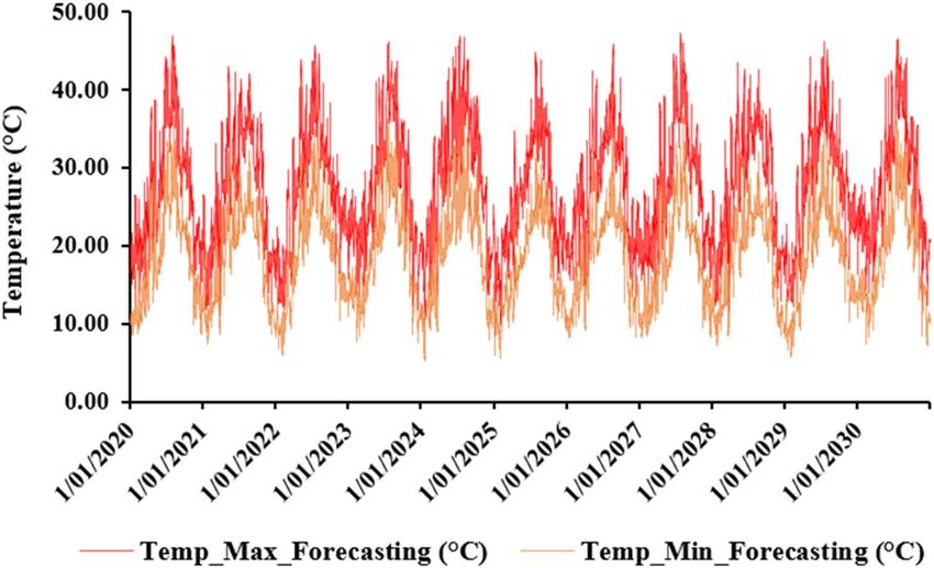
www.nature.com/scientificreports/
Figure 2. Modules and engine of A
PSIM38,53,69,70.
namely: the aridity of the climate, the poor structuring of irrigation water and the salinization of agricultural
land, which limits the development of modern agriculture to high yield.
The map (Fig. 1) was edited using ArcGIS software (10.6 version), based on input vector layers of Moroccan
administrative units (ESRI shapefile format). The input data was downloaded from (www.geodatashp.com).
APSIM model structure and research design. The Agricultural Production Systems sIMulator
(APSIM) is a dynamic farming systems simulation model that combines biophysical and management mod-
ules within a central engine (Fig. 2) on a daily time-step38,49–51. According to Climate K elpie52, APSIM simu-
lates effects of environmental variables and farm management decisions on crop yield and profits. The fact that
APSIM is made out of different soil modules, a range of crop modules and crop management options under dif-
ferent climates makes it an accurate tool for predicting crop yields, if all the data input is done correctly. This also
implies that it can be used everywhere in the world, including in small-scale farming systems of Africa, as long
as it is validated for local conditions and crops. The development of the APSIM model was firstly focused on the
estimation of crop yield as influenced by the availability of water and nitrogen53, but it expanded to include other
agricultural systems and environmental processes54–56. The suite of modules that contains the APSIM software
framework enable the simulation of farming systems for a diverse range of plant57, crop types58, cropping sys-
tems rotations59, management60, soil water61, soil organic carbon62, soil nutrients63, animals64, trees65, climate42,66
and Genotype * Environment * Management interactions67. The simulator is recognized worldwide as a highly
advanced platform for modelling and simulation of agricultural systems68. In this study, the APSIM model v7.10
(www.apsim.info) was used for predicting the wheat yield at different sowing dates, as well as assessing the reli-
ability of the simulations against the measured yield data.
Data input for APSIM. Observed climate data. The daily measured climatic data (rainfall and tempera-
ture) were collected from the meteorological station (32° 15′ 10.2″ N; 7° 57′ 11.9″ W) of National Office of
Agricultural Council (ONCA) in Ben Guerir, while the daily radiation was estimated from solar radiation data
website (www.soda-pro.com). The climate of the Rhamna region is distinguished by apparent variability.
During the period of this study from 2013 to 2019 (i.e., 7 years), the mean annual rainfall of the province is
168 mm; which is low in quantity and erratic in distribution as well. The lowest precipitation is obtained in July
(0.2 mm), whereas the highest is in the month of November, which is 42.24 mm (Fig. 3).
Besides, the annual average daily maximum and minimum temperature are 27.03 °C and 19.12 °C, respec-
tively. August is the hottest month of the year with a maximum and minimum average daily temperature of
37.02 °C and 27.72 °C, respectively. January is therefore the coldest month of the year with a maximum and
minimum average daily temperature in the range respectively of 18.14 °C and 11.37 °C (Fig. 4).
Scientific Reports | (2021) 11:23173 | https://doi.org/10.1038/s41598-021-02668-3 3
Vol.:(0123456789)
www.nature.com/scientificreports/
Figure 3. The evolution of rainfall over 7 years’ time horizon (2013–2019).
Figure 4. The evolution of maximum and minimum temperature over 7 years’ time horizon (2013–2019).
With regard to radiation, Fig. 5 shows the daily solar radiation for 7 years. The annual average daily solar
radiation during this period is 19.71 MJ/m2. The highest monthly averaged radiation was detected in June with
a value of 28.15 MJ/m2, and the lowest radiation was in December with a value of 11.21 MJ/m2.
Future climate data. To study natural phenomena, such as those occurring in our environment (e.g., climate
change), repeated observations of everyone in a population, ordered in time and space, are generally used. Two
factors of variability appear on repeated data sets: the variability between observations measured on the same
individual and the variability between the individuals themselves. The mixed model is a statistical approach that
allows the highlight a relationship between the observed response and the explanatory covariates, taking into
account these two types of variation71–74. The general mixed models that will be used in this study, are presented
in (Eq. 1) according to Laird and Ware75 and Littell et al.76.
yi = Xi β + Zi Ui + εi , (1)
where for each individual i, E ( yi | Ui) = Xiβ + ZiUi is the conditional mean of yi given U i, Zi is a matrix n
i × q of
incidence of random effects U i, we assume that Ui ~ N (0, D), where 0 is the vector of dimension q × 1, D is the
covariance matrix of u. We suppose that u and ε are independent. We still have the variance of y conditionally
to u is Var ( yi | Ui) = Var (εi) = Ri.
Scientific Reports | (2021) 11:23173 | https://doi.org/10.1038/s41598-021-02668-3 4
Vol:.(1234567890)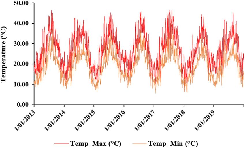
www.nature.com/scientificreports/
Figure 5. The evolution of solar radiation over 7 years’ time horizon (2013–2019).
Based on the graph, all the months show the same behavior over time, which reflects one of the limitations
of the fixed-effects model, which assumes independence between observations. To consider the dependence and
the hierarchical structure of the data, we add a random effect to the fixed-effects model, the model thus obtained
is called a multilevel mixed-effects model.
• For temperature and radiation
(2)
Yijkm = β0 + β1 ∗ A + β2 ∗ B + β3 ∗ C + β4 ∗ D + b0i + b0 j i + b0 jk i + εijkm
β0, β1, β2, β3 and β4 represent the fixed effects. εijkm represents the random, the index i indicates the level
1 observations, j level 2 and k those of level 3, Tijkm is then the kth observation of the temperature/radiation
variable for the day (i) in the month (j) in the year (k), β0 represents the “standard” or average temperature/
radiation of a day at the starting time (Zero Time). The term b0i constitutes the random effect specifying the
day i associated with the intercept and representing the variations in the temperature/radiation of the day with
respect to the start time. The term b0(j)i constitutes the random effect specifying the month j including the day
i associated with the intercept. The term b0(jk)i constitutes the random effect specifying the year k and month
j including the day i associated with the intercept.
A = Time, B = Maxt, C = Mint & D = rainfall.
• For precipitation
(3)
Tijk = β0 + β1 ∗ cos ∗ wXijk−φT + b0i + b0 j i + εijk
With: w = 0.2, ϕT = 20, T and X are fixed, β0, β1 represent fixed effects. The parameters β0, β1 and σε are
estimated by the least squares method.
The subscripts i and j denote respectively the level 1 and 2 observations, Tijk is then the kth observation of
the precipitation variable for month (i) in year (j), β0 corresponds to the "standard" or average precipitation of a
month at the starting time (time zero). The term b0i represents the random effect specifying month (i) associated
with the β0 intercept representing the months precipitation variations from the starting time. The term b0(j)i
is the random effect specifying year j including month i associated with the intercept β0. β1 also represents the
average increase in precipitation per unit time.
Soil data. A survey was carried out to collect both disturbed and undisturbed soil samples from the surface and
subsurface horizons from wheat fields in the Rhamna province. Moreover, field measurement such as soil color
determination was carried out by using a Munsell chart. Furthermore, in accordance with the soil data require-
ment for APSIM model, the physico-chemical soil properties were determined such as texture using a hydrom-
eter according to the B ouyoucos77 method; bulk density (BD) by the core method; soil moisture content by the
gravimetric method; pH-water by the potentiometric method; electrical conductivity (EC) using the EC meter
in a 1:5 soil to water ratio; organic carbon (OC) by the dry combustion; nitrate (NO3−) & ammonium (NH4+) by
the scalar method and cation exchange capacity (CEC) by the cobaltihexamine method.
The study revealed that the soils of Rhamna are dominantly sandy clay loam, reddish brown in color, highly
compacted soil due to a higher bulk density, alkaline pH, non-saline, low in carbon, moderate in nitrogen and
CEC (Table 1).
Scientific Reports | (2021) 11:23173 | https://doi.org/10.1038/s41598-021-02668-3 5
Vol.:(0123456789)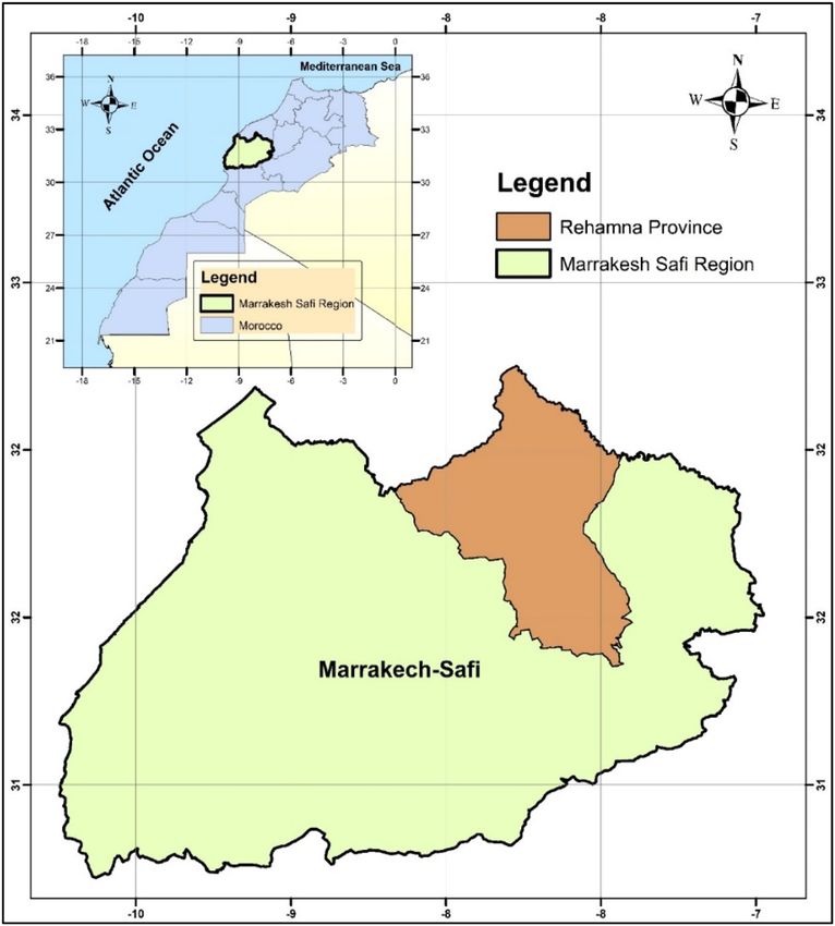
www.nature.com/scientificreports/
CEC
Depth Munsell pH (1:5 EC (1:5 NO3− (kg/ NH4+ (kg/ (cmol + /
(cm) Clay (%) Silt (%) Sand (%) Texture Color BD (g/cm ) SMC (%)
3
water) dS/m) OC (%) ha) ha) kg)
Reddish
Sandy Clay
0–20 20 22 58 Brown 1.45 3.00 8.51 0.54 0.77 14.29 2.35 17.90
Loam
(5YR 4/4)
Reddish
Sandy
20–50 18 20 62 Brown 1.46 3.01 8.53 0.54 0.77 53.15 8.74 18.20
Loam
(5YR 4/4)
Table 1. Soil physical and chemical properties of the Rhamna region.
Evaluation of the APSIM Model. Linear regression was used to compare graphically and to analyze sta-
tistically measured and predicted data of wheat yield, in order to evaluate the adaptability and the performance
of the APSIM model. The statistical indices which are the coefficient of determination (R2), the root mean square
error (RMSE) [Eq. 4], the Nash–Sutcliffe efficiency (NSE)78 [Eq. 5] and the index of agreement (d)79 [Eq. 6], are
defined as follows:
n
0.5
sim 2
Yobs i − Yi
RMSE = (4)
n
i=1
n
obs
2
Y − Ysim
NSE = 1 − i=1
i i
(5)
n obs mean 2
i=1 Yi − Y
sim 2
n
obs
i=1 Yi − Yi
d = 1 −
(6)
n
sim − Ymean
+
Yobs − Ymean
2
i=1 Yi i
where Yi sim is the predicted value, Yi obs is the observed value, Ymean is the mean of the observed values and n is
the number of observations.
For good model performance, values of RMSE [Eq. 4] should be close to 0, that indicate the better agreement
between the two variables80. The agreement value of 1 indicates a perfect match of the simulated to the observed
data for NSE [Eq. 5]78 and d [Eq. 6]81. Vice versa, 0 indicates no agreement for both.
Model validation. Various simulations for wheat yield were conducted by APSIM model Version 7.10
under natural rainfed conditions for Marzak cultivar, which is the common variety mostly used in the Rhamna
region—Central Morocco. They were carried out using: (i) a daily weather data for 7 years (2013 to 2019), (ii)
soil data, (iii) water balance parameters calculated and/or estimated as described by/in previous s tudies82–90, and
(iv) growth and management crop data retrieved from the field survey. In fact, a calibration of the APSIM model
was realized until obtaining a simulated wheat yield that fully matches with the measured wheat yield of Rhamna
region, which were collected from the Regional Office for Agricultural Development of Haouz, Morocco (ORM-
VAH). Indeed, the projected climate data (2020 to 2030) which is realized by the statistical mixed model was
integrated in the calibrated APSIM model to obtain the future scenarios of wheat yield. Therefore, different sow-
ing dates were simulated using the calibrated APSIM model to analyze their effects on wheat yield. Wheat may
be sown early due to the limitation of the available water, and it may be sown at a medium or late date due to
delay in harvesting previous crops and/or rainfall. However, according to the regional sowing window, the sow-
ing dates started on 25 October and were repeated every 10 days until 5 January. Moreover, several simulations
with various varieties of wheat under the same conditions were analyzed to choose the most suitable cultivar for
the region with high yield.
Results
Climate change scenarios. Adjustment of the model (2). The fitting of the second model gives the fol-
lowing results (Fig. 6):
According to the synthesis results, the p-value is lower than 0.05 for all parameters of the fixed effect of radia-
tion, temperature and rain. Therefore, the obtained values for the random effect and error parameters agree.
Thus, to assert the validation of the model, we need to examine the fit of the fitted values and errors, and to
check the normal distribution line: The points are well fitted by contribution to normality, and the samples follow
the normal distribution by perfection. Thus, the measurement errors are also aligned in terms of mean (Figs. 7,
8, 9). Therefore, the multilevel linear mixed effect model is suitable for the sample we want to treat.
Adjustment of the model (3).. Consistent with the simulation results, the p-value is also less than 0.05 for all
precipitation fixed effect parameters (Fig. 10). Furthermore, the values obtained for the random effect and error
parameters are consistent.
Scientific Reports | (2021) 11:23173 | https://doi.org/10.1038/s41598-021-02668-3 6
Vol:.(1234567890)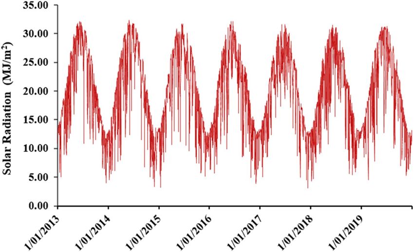
www.nature.com/scientificreports/

                                  Figure 6.  Summary of the model (2).

                                  Figure 7.  Radiation in terms of the adjusted values.

                                      Furthermore, to affirm the validation of the model, we need to examine the fit of the fitted values and errors,
                                  and check the normal distribution line: The points are well fitted with respect to normality. Thus, the measure-
                                  ment errors are also aligned in terms of mean (Figs. 11, 12). Therefore, the multilevel linear mixed effect model
                                  is suitable for the sample we want to treat.

                                  Future scenarios. The results of future scenarios for the Rhamna region from 2020 to 2030 showed that the
                                  mean annual rainfall is about 113 mm, which is low in quantity and erratic in distribution as well. The low-
                                  est precipitation is obtained in June (0.05 mm), whereas the highest is in the month of November, which is
                                  35.84 mm (Fig. 13).

Scientific Reports |   (2021) 11:23173 |               https://doi.org/10.1038/s41598-021-02668-3                                                  7

                                                                                                                                              Vol.:(0123456789)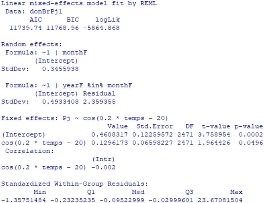
www.nature.com/scientificreports/
Figure 8. Errors in terms of the adjusted values.
Figure 9. The standard Normal.
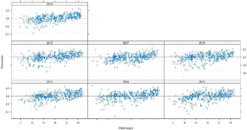
The annual average daily maximum and minimum temperature are 27.61 °C and 18.67 °C, respectively.
August is the hottest month of the year, with a maximum and minimum average daily temperature of 37.50 °C
and 27.20 °C, respectively. January is therefore the coldest month of the year with a maximum and minimum
average daily temperature in the range respectively of 18.86 °C and 11.11 °C (Fig. 14).
Figure 15 shows the daily solar radiation for the future years (2020–2030). The annual average daily solar
radiation during this period is 18.61 MJ/m2. The highest monthly averaged radiation was detected in June with
a value of 27.06 MJ/m2, and the lowest radiation was in December with a value of 10.09 MJ/m2.
Performance of APSIM model. To assess whether the model provided the right answer (wheat yield)
for the right reasons, we compared the wheat yield measurements for 6 years to APSIM simulations output
(Table 2; Fig. 16). Three parameters are found to be the most sensitive with the relative sensitivity values such as:
Scientific Reports | (2021) 11:23173 | https://doi.org/10.1038/s41598-021-02668-3 8
Vol:.(1234567890)
www.nature.com/scientificreports/

                                  Figure 10.  Summary of the model (3).

                                  Figure 11.  Precipitation in terms of the adjusted values.

                                  photoperiod, vernalization and the initial fraction of plant available water capacity (PAWC). We found that after
                                  determining these three coefficients, the model predicted well the wheat yield in the Rhamna region—Central
                                  Morocco.
                                     According to the performance criteria, the simulated data of wheat yield by APSIM model in comparison
                                  with the observed data allowed us to obtain a good model performance with very satisfactory values of RMSE,
                                  NSE and d of the order of 0.13, 0.95 and 0.98, respectively (Table 2; Fig. 16).
                                     Therefore, the aforementioned indexes imply the robustness of the model in predicting wheat yield. They
                                  demonstrated that the APSIM-wheat model provided an excellent simulation performance during the deter-
                                  mination of winter wheat yield for the Rhamna region. This indicates that the model can reflect the reality and
                                  provides a better estimation of the studied process.

                                  Future scenarios for wheat yield.        Various simulations were achieved using the calibrated APSIM model
                                  to estimate the wheat yield of Marzak cultivar for the future scenarios in the Rhamna region. The results show
                                  that the yield varies between 0 and 2.33 t/ha throughout the study period (Fig. 17). The maximum yield was
                                  observed for the 2026–2027 season, and the minimum yield was observed for five seasons that are: 2019–2020,
                                  2020–2021, 2022–2023, 2025–2026, 2029–2030. The two seasons, 2023–2024 and 2027–2028, show yields

Scientific Reports |   (2021) 11:23173 |               https://doi.org/10.1038/s41598-021-02668-3                                                9

                                                                                                                                            Vol.:(0123456789)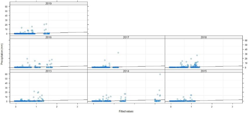
www.nature.com/scientificreports/

                                            Figure 12.  Errors in terms of the adjusted values.

                                            Figure 13.  The evolution of rainfall over future years (2020–2030).

                                            between 1 and 2 t/ha (1.14 t/ha and 1.50 t/ha, respectively). The yields for the three last seasons (2021–2022,
                                            2024–2025 and 2028–2029) are between 0 and 1 t/ha (0.54 t/ha, 0.91 t/ha and 0.70 t/ha, respectively).
                                                The seasons that present a zero or minimal yield are consistent with the seasons in which the rainfall is limited
                                            or insufficient. In general, the yield still not satisfactory since the area is characterized by a semi-arid climate.

                                            Optimum sowing date of wheat.               In the Rhamna region, there is no standard planting date, each farmer
                                            plants wheat crop on a date that suits him. Some of them are sown early, others during the medium or late period.
                                                In this context, different simulation was carried out by the calibrated APSIM model to determine the opti-
                                            mum sowing date in the Rhamna region for the wheat crop, which was strongly affected by weather conditions
                                            and sowing date.
                                                Figure 18 shows that the highest yield was simulated during the early and medium sowing date of agricultural
                                            seasons, which are 25 October and 25 November, respectively. The highest yields during early sowing date were
                                            observed in four seasons, which are: 2021–2022, 2024–2025, 2027–2028 and 2028–2029. Besides, the highest
                                            yields during medium sowing date were spotted in two seasons: 2023–2024 and 2026–2027.
                                                The agricultural season of 2021–2022 ranged from 0.29 to 1.38 t/ha, the highest and lowest yields were simu-
                                            lated for 25 October and 5 January sowing dates, respectively. Delaying the sowing date from 25 October to 5
                                            January decreased yield of 1.09 t/ha. Further, the maximum value brought about in an increase in yield of 0.84
                                            t/ha in comparison with the yield of the same season simulated by APSIM model.
                                                Regarding the agricultural season of 2024–2025, the yields varied from 0.76 to 2.32 t/ha which were predicted
                                            for 5 January and 25 October, respectively. The yield decreased by approximately 1.56 t/ha, with a delay in the

          Scientific Reports |   (2021) 11:23173 |               https://doi.org/10.1038/s41598-021-02668-3                                                   10

Vol:.(1234567890)
www.nature.com/scientificreports/
Figure 14. The evolution of maximum and minimum temperature over future years (2020–2030).
Figure 15. The evolution of solar radiation over future years (2020–2030).
Grain yield (t/ha)
Cropping year Measured Simulated
2013–2014 1.66 1.44
2014–2015 0.26 0.27
2015–2016 0.05 0.00
2016–2017 1.06 1.27
2017–2018 0.45 0.35
2018–2019 0.02 0.00
Index
R2 0.95
RMSE 0.13
NSE 0.95
d 0.98
Table 2. Statistical indices of assessing the performance of APSIM-Wheat model in predicting grain yield.
Scientific Reports | (2021) 11:23173 | https://doi.org/10.1038/s41598-021-02668-3 11
Vol.:(0123456789)www.nature.com/scientificreports/
Figure 16. Predicted versus measured wheat yield of Marzak cultivar.
Figure 17. Future scenarios for wheat yield in the Rhamna region.
sowing date from 25 October to 5 January. In addition, the maximum value brought about an increase in yield
of about 1.41 t/ha in comparison with the yield of the same year.
Concerning the year of 2027–2028, the yield ranged from 0.10 to 2.05 t/ha. The lowest yield was noticed
through sowing on 5 January, and the highest yield through sowing on 25 October. Delay in sowing date from
25 October to 5 January has resulted in a decrease in yield with about 1.95 t/ha. Besides, the maximum yield
obtained showed an increase in comparison with the yield of the same year with a value of 0.55 t/ha.
Relating to the average predicted yield for the year of 2028–2029, it varied from 0.32 to 1.69 t/ha. Minimum
and maximum yields were simulated for 5 January and 25 October sowing dates, respectively. Delay in sowing
date from 25 October to 5 January resulted in a yield diminution of about 1.37 t/ha. Furthermore, the maximum
yield obtained showed an increase in comparison with the yield of the same season with a value of 0.99 t/ha.
Otherwise, the agricultural season of 2023–2024 ranged from 0.40 to 1.17 t/ha, the highest and lowest yields
were simulated for 25 November and 5 January sowing dates, respectively. Delaying the sowing date from 25
November to 5 January decreased yield of 0.77 t/ha. In addition, the maximum value brought about an increase
in yield of 0.03 t/ha in comparison with the yield of the same season simulated by the APSIM model.
Moreover, the agricultural season of 2026–2027 varied from 0.78 to 2.72 t/ha which were predicted for 5 Janu-
ary and 25 November, respectively. The yield decreased by approximately 1.94 t/ha, with a delay in the sowing
Scientific Reports | (2021) 11:23173 | https://doi.org/10.1038/s41598-021-02668-3 12
Vol:.(1234567890)www.nature.com/scientificreports/
Figure 18. Predicted yield for different sowing dates of Marzak cultivar for the future scenarios.
date from 25 November to 5 January. Also, the maximum value resulted in an increase in yield of about 0.39 t/
ha in comparison with the yield of the same season.
On the other hand, the four seasons that are 2020–2021, 2022–2023, 2025–2026 and 2029–2030 do not give
significant results because they corresponded to years of drought, especially during the growing period, which
led to multiple impacts on wheat yield.
Wheat varieties. After the calibration of the APSIM model, different scenarios were carried out under
the same conditions by comparing the yield of other varieties with the yield of the Marzak cultivar used in the
Rhamna region.
The varieties which exhibited maximum values compared to the Marzak variety are presented in Fig. 19 dur-
ing the calibration period, and in Fig. 20 during the future scenarios period.
Scientific Reports | (2021) 11:23173 | https://doi.org/10.1038/s41598-021-02668-3 13
Vol.:(0123456789)www.nature.com/scientificreports/
Figure 19. Comparison of several varieties simulated at the same conditions of the study area for the calibrated
period (2014–2019).
Figure 20. Comparison of several varieties simulated at the same conditions of the study area for the future
scenarios (2020–2030).
The maximum value resulted from scenarios of cultivars for the calibration period (Fig. 19) was observed on
two varieties of wheat, which are Hartog and Sunstate. The minimum and maximum value for the two cultivars
varied from 1.86 to 4.57 t/ha, respectively. The highest and lowest yield was increased by values of 3.13 t/ha and
1.55 t/ha compared to Marzak cultivar, respectively. Also, the Batten variety ranged from 1.81 to 3.86 t/ha. These
values show an increase of 1.5 and 2.42 t/ha, respectively. Regarding Wollaroi, it varied between 1.84 and 3.78
t/ha, which shows an increase of 1.53 and 2.34 t/ha, respectively. Moreover, Sapphire reaches maximum values
relative to the crop used in the region which ranged between 2.19 and 3.71 t/ha. These values show an increase
of 1.88 and 2.27 t/ha, respectively.
Similarly, as calibration period, Hartog and Sunstate cultivars show also maximum value during the future
scenarios period (Fig. 20). The minimum and maximum value for the two cultivars varied from 2.07 to 4.49 t/
ha, respectively. The highest and lowest yield was increased by values of 2.16 t/ha and 1.53 t/ha compared to
Scientific Reports | (2021) 11:23173 | https://doi.org/10.1038/s41598-021-02668-3 14
Vol:.(1234567890)www.nature.com/scientificreports/
Marzak cultivar, respectively. As regards the Batten variety, it ranged from 2.39 to 4.44 t/ha. These values show
an increase of 1.85 and 2.11 t/ha, respectively. Furthermore, Sapphire cultivar varied between 2.25 and 4.26 t/ha.
These values show an increase of 1.71 and 1.93 t/ha, respectively. Furthermore, Wollaroi variety ranged between
1.93 and 3.90 t/ha, which shows an increase of 1.39 and 1.57 t/ha, respectively.
These results showed us that the use of one of these varieties in the Rhamna region instead of Marzak cultivar
could lead to a very satisfactory increase in wheat yield.
Discussion
Our results showed that APSIM-Wheat model can be used as a suitable tool to investigate farm productivity thru
building various scenarios management options for optimizing wheat yield under water limited environment.
The ability of APSIM-Wheat model to predict yield in the semi-arid environment was confirmed by previous
studies91–95. Application of APSIM-Wheat for grain yield simulation showed reasonable predictive results not
only in semi-arid climate43,46,96–99, but also in arid44,45,100 and Mediterranean41,42,101–103 environments.
Determining future projections of climate d ata71–76 and integrating them into the APSIM model allowed
us to get future scenarios of wheat yield in the study area. However, low yield was obtained comparing it with
previous years due to either insufficient or absence of rainfall. The production of cereals in the semi-arid areas
of Morocco, such as in other regions with the same climatic conditions, is strongly affected by inadequate or
poorly distributed rainfall91,104. The upsurge of minimum/maximum temperature has been noticed during the
recent decades105. The rise of temperature in the future years will lead to global warming thereby exasperating
the drought incidence and affecting the precipitation pattern. This trend of climate variability justifies that the
damage to agriculture and water scarcity has already been started and will be proliferated further over the next
few years. Similar projections were reported on future climate which carried out using various climate models
including multilevel mixed-effects model in the Moroccan c ontext74,106–111, as well as Northern A frica112–114.
For this reason, various simulations were done to determine the optimum sowing date for the moisture deific
area of Morocco. Accordingly, the simulated result confirmed that the yield obtained from plots seeded between
25 October and 25 November was higher than that sown until 05 January. The relationship between grain yield
and different sowing dates of wheat are linear. The highest Predicted grain yield was obtained when it is sown
in early sowing (i.e., late October) or medium sowing (i.e., late November), and decreased thereafter. The lowest
grain yield was obtained in late sowing (January). This coincides with the findings of researches which affirmed
that both early and medium sowing were beneficial for obtaining a highest yield, but the early sowing was more
favorable to increase the wheat y ield21–26. In addition, the results of predictions of the effect of sowing date on
wheat yield using APSIM model were also consistent with many of the findings of simulations using other crop
models in the semi-arid e nvironment34,115–118. Therefore, extended life duration and favorable temperature espe-
cially at the grain filling stage, might be the main reason for the higher grain yield in early sowing d ates43,119,120.
While, delaying the sowing date beyond the optimum sowing date led to reduced grain yield, due to a shorter
vegetative growth period of w heat115,121. Thus, sowing at the appropriate time can enhance the effective accumula-
tive temperature, prolong the effective growth period of wheat, and then increase the yield122–124.
On the other hand, other simulations were performed using the calibrated APSIM model to test other types
of cultivars, and then analyze and compare their yields with the yield of Marzak cultivars under the same condi-
tions. From several varieties, Hartog, Sunstate, Wollaroi, Batten and Sapphire presented the highest yields in
comparison with the Marzak variety. These significant results were observed for both periods, the calibration
period and the future scenarios period. However, Sunstate and Hartog are the most cultivars adopted in arid and
semi-arid regions, and widely used in these environments for many reasons: (i) very adequate for dry growing
season, (ii) slow variety with excellent yield potential, (iii) did not suffer grain yield or grain quality losses, (iv)
and possess a large resistance to herbicides and root r ot125–130. Moreover, Batten and Sapphire are among the best
performing varieties and among the earlier sown crops with highest yielding in arid and semi-arid climate131,132
but not suitable for the humid and sub-humid r egions133–135. Furthermore, Wollaroi cultivar also performs well
in drier areas, reputed for its high grain quality, tolerance to weathering, and resistance to crown rot and stripe
rust136–140. This indicates that these cultivars are suitable and appropriate for our situation, and the import and
the seed of them increase and enhance the wheat yield in the Rhamna region.
Conclusion
Famers in Morocco continue growing wheat although its productivity is challenged by low and erratic precipita-
tion; hot temperature; poor soil fertility and others. Seemingly, these production factors will aggravate in the years
to come due to climate change. This study concluded that the use of APSIM model can help in evaluating the
suitability of Central Morocco for wheat production. Based on this model, suitable time window for sowing and
promising wheat varieties were identified that can be grown well in water deficit areas. This study recommends
undertaking additional research taking into account varieties, sowing date, supplemental irrigation and nutrient
and best management practices under water stressed environment. Yet, cultivar, sowing time and climate are
found to be the critical factors for wheat growth hence they should be well managed.
Received: 16 July 2021; Accepted: 22 November 2021
References
1. FAO. Food and Agriculture Organization of the United Nations. FAOSTAT Data; www.faostat.fao.org (last access 15.06.21),
(2016).
Scientific Reports | (2021) 11:23173 | https://doi.org/10.1038/s41598-021-02668-3 15
Vol.:(0123456789)www.nature.com/scientificreports/
2. Gomez, D., Salvador, P., Sanz, J. & Casanova, J. L. Modelling wheat yield with antecedent information, satellite and climate data
using machine learning methods in Mexico. Agric. For. Meteorol. 300, 108317. https://doi.org/10.1016/j.agrformet.2020.108317
(2021).
3. Wrigley, C. W. Wheat: A unique grain for the world. In Wheat chemistry and technology 4th edn (eds Khan, K. & Shewry, P. R.)
1–17 (AACC Int. Inc, St Paul, 2009).
4. Awika, J. M. Major cereal grains production and use around the world. In Advances in Cereal Science: Implications to Food
Processing and Health Promotion, Vol. 1089 (eds Awika, J. M., Piironen, V. & Bean, S.) 1–13 (American Chemical Society, 2011).
5. Gupta, R., Meghwal, M. & Prabhakar, P. K. Bioactive compounds of pigmented wheat (Triticum aestivum): Potential benefits in
human health. Trends Food Sci. Technol. 110, 240–252. https://doi.org/10.1016/j.tifs.2021.02.003 (2021).
6. FAO. Food and Agriculture Organization of the United Nations. FAOSTAT Data; www.faostat.fao.org (last access 15.06.21),
(2020).
7. USDA. Grain and Feed Annual. United States Department of Agriculture (USDA), Foreign Agricultural Service (FAS), MO2020-
0007; https://www.fas.usda.gov/data/morocco-grain-and-feed-annual-3 (last access 15.06.21), (2020).
8. McIntyre, C. L. et al. Molecular detection of genomic regions associated with grain yield and yield-related components in an
elite bread wheat cross evaluated under irrigated and rainfed conditions. Theor. Appl. Genet. 120, 527–541. https://doi.org/10.
1007/s00122-009-1173-4 (2010).
9. UN. World population prospects. United Nations (UN), Department of Economic and Social Affairs (DESA); https://www.un.
org/development/desa/en/news/population/world-population-prospects-2017.html (last access 15.06.21), (2017).
10. Gomez-Macpherson, H. & Richards, R. A. Effect of sowing time on yield and agronomic characteristics of wheat in south-eastern
Australia. Aust. J. Agric. Res. 46, 1381–1399. https://doi.org/10.1071/AR9951381 (1995).
11. Stone, P. J. & Nicolas, M. E. Effect of timing of heat stress during grain filling on two wheat varieties differing in heat tolerance.
I. Grain growth. Aust. J. Plant Physiol. 22, 927–934. https://doi.org/10.1071/PP9950927 (1995).
12. Mahdi, L., Bell, C. J. & Ryan, J. Establishment and yield of wheat (Triticum turgidum L.) after early sowing at various depths in
a semi-arid Mediterranean environment. Field Crops Res. 58, 187–196. https://doi.org/10.1016/S0378-4290(98)00094-X (1998).
13. Radmehr, M., Ayeneh, G. A. & Mamghani, R. Responses of late, medium and early maturity bread wheat genotypes to different
sowing date. I. Effect of sowing date on phonological, morphological, and grain yield of four breed wheat genotypes. Iran. J.
Seed. Sapling 21, 175–189 (2003).
14. Turner, N. C. Agronomic options for improving rainfall use efficiency of crops in dryland farming systems. J. Exp. Bot. 55,
2413–2425. https://doi.org/10.1093/jxb/erh154 (2004).
15. Pickering, P. A. & Bhave, M. Comprehensive analysis of Australian hard wheat cultivars shows limited puroindoline allele
diversity. Plant Sci. 172, 371–379. https://doi.org/10.1016/j.plantsci.2006.09.013 (2007).
16. Zheng, B., Chenu, K., Fernanda Dreccer, M. & Chapman, S. C. Breeding for the future: What are the potential impacts of future
frost and heat events on sowing and flowering time requirements for Australian bread wheat (Triticum aestivium) varieties?.
Glob. Change Biol. 18, 2899–2914. https://doi.org/10.1111/j.1365-2486.2012.02724.x (2012).
17. Wu, X. S., Chang, X. P. & Jing, R. L. Genetic insight into yield-associated traits of wheat grown in multiple rain-fed environments.
PLoS ONE 7, e31249. https://doi.org/10.1371/journal.pone.0031249 (2012).
18. Mueller, B. et al. Lengthening of the growing season in wheat and maize producing regions. Weather Clim. Extrem. 9, 47–56.
https://doi.org/10.1016/j.wace.2015.04.001 (2015).
19. Hunt, J. R., Hayman, P. T., Richards, R. A. & Passioura, J. B. Opportunities to reduce heat damage in rainfed wheat crops based
on plant breeding and agronomic management. Field Crops Res. 224, 126–138. https://doi.org/10.1016/j.fcr.2018.05.012 (2018).
20. Ababaei, B. & Chenu, K. Heat shocks increasingly impede grain filling but have little effect on grain setting across the Australian
wheatbelt. Agric. For. Meteorol. 284, 107889. https://doi.org/10.1016/j.agrformet.2019.107889 (2020).
21. Anderson, W. K. & Smith, W. R. Yield advantage of two semi-dwarf compared with two tall wheats depends on sowing time.
Aust. J. Agric. Res. 41, 811–826. https://doi.org/10.1071/AR9900811 (1990).
22. Connor, D. J., Theiveyanathan, S. & Rimmington, G. M. Development, growth, water-use and yield of a spring and a winter
wheat in response to time of sowing. Aust. J. Agric. Res. 43, 493–516. https://doi.org/10.1071/AR9920493 (1992).
23. Owiss, T., Pala, M. & Ryan, J. Management alternatives for improved durum wheat production under supplemental irrigation
in Syria. Eur. J. Agron. 11, 255–266. https://doi.org/10.1016/S1161-0301(99)00036-2 (1999).
24. Bassu, S., Asseng, A., Motzo, R. & Giunta, F. Optimizing sowing date of durum wheat in a variable Mediterranean environment.
Field Crops Res. 111, 109–118. https://doi.org/10.1016/j.fcr.2008.11.002 (2009).
25. Bannayan, M., Eyshi Rezaei, E. & Hoogenboom, G. Determining optimum sowing dates for rainfed wheat using the precipita-
tion uncertainty model and adjusted crop evapotranspiration. Agric. Water Manag. 126, 56–63. https://doi.org/10.1016/j.agwat.
2013.05.001 (2013).
26. Liang, Y. F. et al. Subsoiling and sowing time influence soil water content, nitrogen translocation and yield of dryland winter
wheat. Agronomy 9, 37. https://doi.org/10.3390/agronomy9010037 (2019).
27. Farooq, M., Basra, S. M. A., Rehman, H. & Saleem, B. A. Seed priming enhances the performance of late sown wheat (Triticum
aestivum L.) by improving chilling tolerance. J. Agron. Crop Sci. 194, 55–60. https://doi.org/10.1111/j.1439-037X.2007.00287.x
(2008).
28. Kudair, I. M. & Adary, A. H. The effects of temperature and planting depth on coleoptile length of some Iraqi local and introduced
wheat cultivars. Mesopotamia J. Agric. 17, 49–62 (1982).
29. Leoncini, E. et al. Phytochemical profile and nutraceutical value of old and modern common wheat cultivars. PLoS ONE 7,
e45997. https://doi.org/10.1371/journal.pone.0045997 (2012).
30. Busko, M. et al. The effect of Fusarium inoculation and fungicide application on concentrations of flavonoids (apigenin, kaemp-
ferol, luteolin, naringenin, quercetin, rutin, vitexin) in winter wheat cultivars. Am. J. Plant Sci. 5, 3727–3736. https://doi.org/10.
4236/ajps.2014.525389 (2014).
31. Bannayan, M., Kobayashi, K., Marashi, H. & Hoogenboom, G. Gene-based modeling for rice: An opportunity to enhance the
simulation of rice growth and development?. J. Theor. Biol. 249, 593–605. https://doi.org/10.1016/j.jtbi.2007.08.022 (2007).
32. Soler, C. M. T., Sentelhas, P. C. & Hoogenboom, G. Application of the CSM-CERES-Maize model for sowing date evaluation
and yield forecasting for maize grown off-season in a subtropical environment. Eur. J. Agron. 18, 165–177. https://doi.org/10.
1016/j.eja.2007.03.002 (2007).
33. Andarzian, B. et al. WheatPot: A simple model for spring wheat yield potential using monthly weather data. Biosyst. Eng. 99,
487–495. https://doi.org/10.1016/j.biosystemseng.2007.12.008 (2008).
34. Andarzian, B., Hoogenboom, G., Bannayan, M., Shirali, M. & Andarzian, B. Determining optimum sowing date of wheat using
CSM-CERES-Wheat model. J. Saudi Soc. Agric. Sci. 14, 189–199. https://doi.org/10.1016/j.jssas.2014.04.004 (2015).
35. Palosuo, T. et al. Simulation of winter wheat yield and its variability in different climates of Europe: A comparison of eight crop
growth models. Eur. J. Agron. 35, 103–114. https://doi.org/10.1016/j.eja.2011.05.001 (2011).
36. Rötter, R. P. et al. Simulation of spring barley yield in different climatic zones of Northern and Central Europe: A comparison
of nine crop models. Field Crops Res. 133, 23–36. https://doi.org/10.1016/j.fcr.2012.03.016 (2012).
37. Ran, H. et al. Capability of a solar energy-driven crop model for simulating water consumption and yield of maize and its
comparison with a water-driven crop model. Agric. For. Meteorol. 287, 107955. https://doi.org/10.1016/j.agrformet.2020.107955
(2020).
Scientific Reports | (2021) 11:23173 | https://doi.org/10.1038/s41598-021-02668-3 16
Vol:.(1234567890)www.nature.com/scientificreports/
38. Keating, B. A. et al. An overview of APSIM, a model designed for farming systems simulation. Eur. J. Agron. 18, 267–288. https://
doi.org/10.1016/S1161-0301(02)00108-9 (2003).
39. Probert, M. E. & Dimes, J. P. Modelling release of nutrients from organic resources using APSIM. In Modelling nutrient manage-
ment in tropical cropping systems Vol. 114 (eds Delve, R. J. & Probert, M. E.) 25–31 (ACIAR Proceedings, 2004).
40. Mohanty, M. et al. Simulating soybean–wheat cropping system: APSIM model parameterization and validation. Agric. Ecosyst.
Environ. 152, 68–78. https://doi.org/10.1016/j.agee.2012.02.013 (2012).
41. George, N., Thompson, S. E., Hollingsworth, J., Orloff, S. & Kaffka, S. Measurement and simulation of water-use by canola and
camelina under cool-season conditions in California. Agric. Water Manag. 196, 15–23. https://doi.org/10.1016/j.agwat.2017.
09.015 (2018).
42. Bahri, H., Annabi, M., M’Hamed, H. C. & Frija, A. Assessing the long-term impact of conservation agriculture on wheat-based
systems in Tunisia using APSIM simulations under a climate change context. Sci. Total Environ. 692, 1223–1233. https://doi.
org/10.1016/j.scitotenv.2019.07.307 (2019).
43. Ahmed, M. et al. Novel multimodel ensemble approach to evaluate the sole effect of elevated C O2 on winter wheat productivity.
Sci. Rep. 9, 7813. https://doi.org/10.1038/s41598-019-44251-x (2019).
44. Eyni-Nargeseh, H., Deihimfard, R., Rahimi-Moghaddam, R. & Mokhtassi-Bidgoli, A. Analysis of growth functions that can
increase irrigated wheat yield under climate change. Meteorol. Appl. 27, 1–10. https://doi.org/10.1002/met.1804 (2020).
45. Rahimi-Moghaddam, S., Eyni-Nargeseh, H., Kalantar Ahmadi, S. A. & Azizi, K. Towards withholding irrigation regimes and
resistant genotypes as strategies to increase canola production in drought-prone environments: A modeling approach. Agric.
Water Manag. 243, 106487. https://doi.org/10.1016/j.agwat.2020.106487 (2021).
46. Berghuijs, H. N. C. et al. Calibrating and testing APSIM for wheat-faba bean pure cultures and intercrops across Europe. Field
Crops Res. 264, 108088. https://doi.org/10.1016/j.fcr.2021.108088 (2021).
47. METLE. National Report. Ministry of Equipment, Transport, Logistics and Water (last access 15.06.21), (2019).
48. HCP. Voluntary national review of the implementation of the sustainable development goals. High Comm. Plng. p. 188 (2020).
49. Hammer, G. L. et al. Adapting APSIM to model the physiology and genetics of complex adaptive traits in field crops. J. Exp. Bot.
61, 2185–2202. https://doi.org/10.1093/jxb/erq095 (2010).
50. Holzworth, D. P. et al. APSIM—evolution towards a new generation of agricultural systems simulation. Environ. Model. Softw.
62, 327–350. https://doi.org/10.1016/j.envsoft.2014.07.009 (2014).
51. Gaydon, D. S. et al. Evaluation of the APSIM model in cropping systems of Asia. Field Crops Res. 204, 52–75. https://doi.org/
10.1016/j.fcr.2016.12.015 (2017).
52. Climate Kelpie website. http://w ww.c limat ekelp
ie.c om.a u/m
anage-c limat e/d
ecisi on-s uppor t-t ools-f or-m
anagi ng-c limat e (2010).
53. McCown, R. L., Hammer, G. L., Hargreaves, J. N. G., Holzworth, D. P. & Freebairn, D. M. APSIM: A novel software system for
model development, model testing and simulation in agricultural systems research. Agric. Syst. 50, 255–271. https://doi.org/10.
1016/0308-521X(94)00055-V (1996).
54. Cichota, R., Vogeler, I., Werner, A., Wigley, K. & Paton, B. Performance of a fertiliser management algorithm to balance yield
and nitrogen losses in dairy systems. Agric. Syst. 162, 56–65. https://doi.org/10.1016/j.agsy.2018.01.017 (2018).
55. Laurenson, S., Cichota, R., Reese, P. & Breneger, S. Irrigation runoff from a rolling landscape with slowly permeable subsoils in
New Zealand. Irrig. Sci. 36, 121–131. https://doi.org/10.1007/s00271-018-0570-3 (2018).
56. Rodriguez, D. et al. Predicting optimum crop designs using crop models and seasonal climate forecasts. Sci. Rep. 8, 2231. https://
doi.org/10.1038/s41598-018-20628-2 (2018).
57. Archontoulis, S. V., Miguez, F. E. & Moore, K. J. A methodology and an optimization tool to calibrate phenology of short-day
species included in the APSIM PLANT model: Application to soybean. Environ. Model. Softw. 62, 465e477. https://doi.org/10.
1016/j.envsoft.2014.04.009 (2014).
58. Brown, H., Huth, N. & Holzworth, D. Crop model improvement in APSIM: Using wheat as a case study. Eur. J. Agron. 100,
141–150. https://doi.org/10.1016/j.eja.2018.02.002 (2018).
59. Yang, X. et al. Cropping system productivity and evapotranspiration in the semiarid Loess Plateau of China under future tem-
perature and precipitation changes: An APSIM-based analysis of rotational vs. Continuous systems. Agric. Water Manag. 229,
105959. https://doi.org/10.1016/j.agwat.2019.105959 (2020).
60. Balboa, G. R. et al. A systems-level yield gap assessment of maize-soybean rotation under highand low-management inputs in
the Western US Corn Belt using APSIM. Agric. Syst. 174, 125–154. https://doi.org/10.1016/j.agsy.2019.04.008 (2019).
61. Yang, X. et al. Modelling the effects of conservation tillage on crop water productivity, soil water dynamics and evapotranspira-
tion of a maize-winter wheat-soybean rotation system on the Loess plateau of China using APSIM. Agric. Syst. 166, 111–123.
https://doi.org/10.1016/j.agsy.2018.08.005 (2018).
62. Mohanty, M. et al. Soil carbon sequestration potential in a Vertisol in central India- results from a 43-year long-term experiment
and APSIM modeling. Agric. Syst. 184, 102906. https://doi.org/10.1016/j.agsy.2020.102906 (2020).
63. Vogeler, I., Thomas, S. & van der Weerden, T. Effect of irrigation management on pasture yield and nitrogen losses. Agric. Water
Manag. 216, 60–69. https://doi.org/10.1016/j.agwat.2019.01.022 (2019).
64. Bosi, C. et al. APSIM-tropical pasture: A model for simulating perennial tropical grass growth and its parameterisation for
palisade grass (Brachiaria brizantha). Agric. Syst. 184, 102917. https://doi.org/10.1016/j.agsy.2020.102917 (2020).
65. Smethurst, P. J., Valadares, R. V., Huth, N. I., Almeida, A. C. & Júlio, C. L. N. Generalized model for plantation production of
Eucalyptus grandisand hybrids forgenotype-site-management applications. For. Ecol. Manag. 469, 118164. https://doi.org/10.
1016/j.foreco.2020.118164 (2020).
66. Xiao, D. P., Liu, D. L., Wang, B., Feng, P. Y. & Tang, J. Z. Climate change impact on yields and water use of wheat and maize in
the north China plain under future climate change scenarios. Agric. Water Manag. 238, 1–15. https://doi.org/10.1016/j.agwat.
2020.106238 (2020).
67. Seyoum, S., Rachaputi, R., Chauhan, Y., Prasanna, B. & Fekybelu, S. Application of the APSIM model to exploit G × E × M
interactions for maize improvement in Ethiopia. Field Crops Res. 217, 113–124. https://doi.org/10.1016/j.fcr.2017.12.012 (2018).
68. Basche, A. D. & DeLonge, M. S. Comparing infiltration rates in soils managed with conventional and alternative farming meth-
ods: A meta-analysis. PLoS ONE 14, e0215702. https://doi.org/10.1371/journal.pone.0215702 (2019).
69. Holzworth, D. et al. The development of a farming systems model (APSIM): A disciplined approach. In Proceedings of the iEMSs
Third Biennial Meeting, Burlington, VT, USA, 9–13 July 2006 (International Environmental Modelling and Software Society,
Manno, Switzerland, 2006).
70. Gaydon, D. S. The APSIM model—an overview. In SAC Monograph: The SAARC-Australia Project Developing Capacity in Crop-
ping Systems Modelling for South Asia (eds Dr. Donald S. Gaydon et al.) 15–31 (2014).
71. Pinheiro, J. C. & Bates, D. M. Mixed Effects Models in S and S-Plus (Statistics and Computing) (Springer, New York, 2000).
72. El Halimi, R. Nonlinear Mixed-effects Models and Bootstrap resampling: Analysis of Non-normal Repeated Measures in Bio-
statistical Practice. Amazon Books. 320 (2009).
73. Vock, D. M., Davidian, M., Tsiatis, A. A. & Muir, A. J. Mixed model analysis of censored longitudinal data with flexible random-
effects density. Biostat. 13, 61–73. https://doi.org/10.1093/biostatistics/kxr026 (2012).
74. Beroho, M. et al. Analysis and prediction of climate forecasts in Northern Morocco: Application of multilevel linear mixed
effects models using R Software. Heliyon 6, e05094. https://doi.org/10.1016/j.heliyon.2020.e05094 (2020).
Scientific Reports | (2021) 11:23173 | https://doi.org/10.1038/s41598-021-02668-3 17
Vol.:(0123456789)You can also read