Working Paper Heterogeneity within the Euro Area: New Insights into an Old Story - CEPII
←
→
Page content transcription
If your browser does not render page correctly, please read the page content below
No 2019-05 – March
                                                Working Paper

                                              Heterogeneity within the Euro Area:
                                                   New Insights into an Old Story
                                              Virginie Coudert, Cécile Couharde, Carl Grekou & Valérie Mignon

Highlights
          This article provides a new framework for assessing the sustainability of the EMU.

          We identify two distinct groups of countries in the run-up to the EMU, Greece being clearly an outlier at that
          time.

          We find that disparities have increased across and within countries’ groups, and that Greece has become
          more peripheral over time.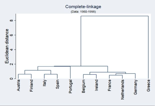
CEPII Working Paper                                                       Heterogeneity within the Euro Area: New Insights into an Old Story

   Abstract
We assess cross-country heterogeneity within the eurozone and its evolution over time by measuring the distances
between the equilibrium exchange rates’ paths of member countries. These equilibrium paths are derived from the
minimization of currency misalignments, by matching real exchange rates with their economic fundamentals. Using
cluster and factor analyses, we identify two distinct groups of countries in the run-up to the European Monetary Union
(EMU), Greece being clearly an outlier at that time. Comparing the results with more recent periods, we find evidence
of rising dissimilarities between these two sets of countries, as well as within the groups themselves. Overall, our
findings illustrate the building-up of macroeconomic imbalances within the eurozone before the 2008 crisis and the
fragmentation between its member countries that followed.

   Keywords
Euro Area, Equilibrium Exchange Rates, Cluster Analysis, Factor Analysis, Macroeconomic Imbalances.

   JEL
F33, F45, E5, C38.

Working Paper

   CEPII (Centre d’Etudes Prospectives et                  CEPII Working Paper                         Editorial Director:   CEPII
   d’Informations Internationales) is a French institute   Contributing to research in international   Sébastien Jean        20, avenue de Ségur
   dedicated to producing independent, policy-             economics                                                         TSA 10726
                                                                                                       Production:           75334 Paris Cedex 07
   oriented economic research helpful to understand
                                                           © CEPII, PARIS, 2019                        Laure Boivin          +33 1 53 68 55 00
   the international economic environment
                                                                                                                             www.cepii.fr
   and challenges in the areas of trade policy,            All rights reserved. Opinions expressed     No ISSN: 1293-2574    Press contact: presse@cepii.fr
   competitiveness, macroeconomics, international          in this publication are those of the
   finance and growth.                                     author(s) alone.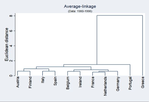
CEPII Working Paper                           Heterogeneity within the euro area: New insights into an old story

                 Heterogeneity within the euro area: New insights into an old story1

                       Virginie Coudert∗ , Cécile Couharde† , Carl Grekou‡ , Valérie Mignon§

1.    Introduction

     The 2008 financial crisis and the sovereign crisis that followed in Europe have revived
debates about the European Monetary Union (EMU). The most lingering question un-
derlying most issues is to know if member states are similar enough to share the same
currency in the long run. Whatever the answer, drastic steps had to be taken rapidly in
2012 to avoid a fragmentation of the eurozone. Monetary policy has largely contributed
to alleviate the diverging pressures, notably though the quantitative easing strategy, en-
largement of collateral and the public sector purchase program (PSPP). Fiscal policy
has also been more tightened in the peripheral countries in order to restore the sustain-
ability of public finances. Besides, banking supervision has been strengthened through
the banking union. On the whole, the functioning of the euro area has been improved
compared to the pre-2008 period.
     Despite all these advances, the key question remains to know if the countries are
reasonably similar to benefit from sharing the same currency and if differences have been
ironed out since the launch of the euro. As pointed out by Lane (2006), this issue was
identified as a major challenge for the success of the euro from its beginning. It led to
numerous contributions in the wake of the Maastricht Treaty that largely focused on
studying convergence in prices and business cycles within the euro area. In particular,
earlier empirical studies typically relied on the optimum currency area (OCA) literature
(Mundell, 1961; McKinnon, 1963; Kenen, 1969), in order to examine whether future
eurozone members meet the OCA criteria that could allow them to be less vulnerable to
1
   Corresponding author : Valérie Mignon, EconomiX-CNRS, University of Paris Nanterre, 200 avenue de
la République, 92001 Nanterre cedex, France. Email: valerie.mignon@parisnanterre.fr.
We are very grateful to Anne-Laure Delatte for valuable comments and suggestions. This paper reflects
the opinions of the authors and does not necessarily express the views of the institutions to which they
belong.
 ∗
   Banque de France, Direction de la Stabilité Financière, Paris, France
 †
   EconomiX-CNRS, University of Paris Nanterre, France
 ‡
   CEPII and EconomiX-CNRS, University of Paris Nanterre, France.
 §
   EconomiX-CNRS, University of Paris Nanterre, and CEPII, Paris, France

                                                       3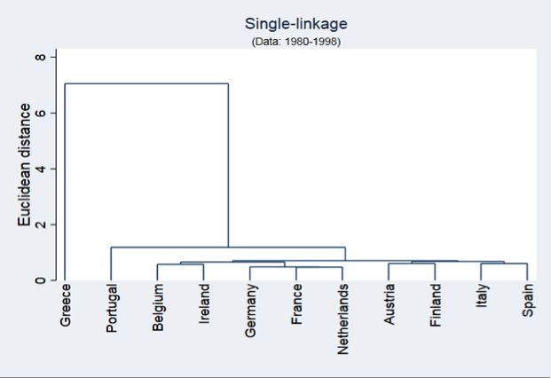
CEPII Working Paper                        Heterogeneity within the euro area: New insights into an old story

       shocks and then to undergo low stabilization costs in joining the EMU.2 The findings of
       this literature usually tended to be pessimistic about the possibility for European coun-
       tries to form a viable monetary union. In particular, in their seminal article, Bayoumi and
       Eichengreen (1993) highlighted the existence of a core–periphery pattern in the run-up
       to the EMU. Using pre-EMU data (1960-88) to estimate the degree of supply shocks
       synchronization, they showed that, over this period, there was a core (Germany, France,
       Belgium, the Netherlands, and Denmark) where shocks were highly correlated, and a
       periphery (Greece, Ireland, Italy, Portugal, Spain, and UK) where synchronization was
       significantly lower. Bayoumi and Eichengreen (1993) suggested that, if persistent, this
       pattern would be detrimental to the EMU project.
            As the single currency seemed to perform successfully until the 2008 crisis despite
       these bleak predictions, some observers criticized the previous analyses on the ground
       that they ignored the complex nature of monetary unification and its endogenous char-
       acter. In particular, Frankel and Rose (1998) presented empirical evidence that countries
       with more bilateral trade will feature higher business cycle correlations. As monetary uni-
       fication induced eurozone members to trade more with each other (see Baldwin (2006)
       for a survey), the process should be matched by an increase in business cycle synchro-
       nization among countries. It would then become easier for euro-area members to meet
       the OCA criteria. The shock caused by the 2007-08 financial collapse, followed by the
       European sovereign debt crisis, has however raised new doubts about the ability of the
       single currency to work well in a region with huge economic and political diversity (see
       Stiglitz, 2017). It has also given a new dimension to this debate by highlighting the
       building-up of unsustainable macroeconomic imbalances within the eurozone.
            The objective of this paper is to revisit such issue of sharing a common currency by
       taking stock of the consensus reached after the 2008 crisis that highlighted the accumu-
       lation of macroeconomic imbalances in the run-up to most financial crises. Specifically,
       we examine between-country disparities in terms of equilibrium exchange rates, i.e., ex-
       change rates that would prevent currency misalignments resulting from unsustainable
       macroeconomic disequilibria within the member countries. We consider the oldest mem-
       bers of the EMU, namely the ten founding members and Greece in order to have a
       long historical record —our sample spanning from 1980 to 2016. First, we assess the
       equilibrium exchange rate paths for the considered euro-area members. Second, we rely
       on a cluster analysis to partition the euro-area countries into homogeneous groups or

        2
         For a survey, see Bayoumi and Eichengreen (1994), De Grauwe (1997), Lafrance and St-Amant (1999),
       and Alesina, Barro and Tenreyro (2002).

                                                   4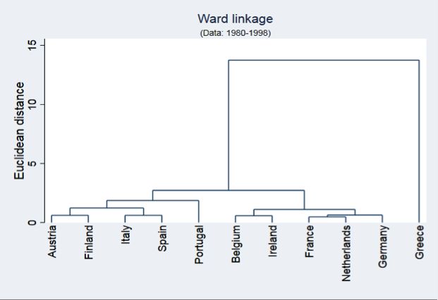
CEPII Working Paper                       Heterogeneity within the euro area: New insights into an old story

clusters in order to measure how equilibrium exchange rate trajectories have been dis-
tant across euro-area members. Third, we try to identify the characteristics of EMU
members that explain the formation of such clusters. In these two last parts, we split
the sample into several sub-periods in order to investigate the dynamics of these clusters
over time thanks to the identification of their main underlying factors, before and after
the monetary union, as well as before and after the 2008 crisis.

     Previewing our main results, we find that that the pre-euro configuration of the eu-
rozone can be partitioned into three groups of countries. On the one hand, Belgium,
France, Germany, Ireland, and the Netherlands form the most homogenous group; on the
other hand, Austria, Finland, Italy, and Spain constitute the second group. We also find
evidence of two outliers, namely Portugal and Greece. Indeed, these countries exhibit
the most divergent equilibrium exchange rate paths; Greece being the most idiosyncratic
country. The comparison with the post-euro period reveals that member states have not
moved structurally closer to each other. On the contrary, we find that (i) disparities have
increased across and within countries’ groups, and (ii) Greece has moved away from the
other member states, becoming more peripheral over time. Only Spain seems to gradu-
ally converge towards the core countries. Overall, our findings point out the disparities
within the euro area and their evolution through time.
     The rest of the paper is structured as follows. Section 2 describes our methodological
framework to assess equilibrium exchange rates. Section 3 presents the partition of the
euro area based on cluster analysis, while that issued from factor analysis is analyzed
in Section 4. In both sections, we make the distinction between the period before and
after the implementation of the EMU to get evidence of the build-up of macroeconomic
imbalances within the euro area. Finally, Section 5 concludes.

2.     Equilibrium exchange rates within the euro area

2.1.    The relevance of currency misalignments inside the monetary union

     There is common sense among economists and policymakers that currency misalign-
ments—i.e., departures of real exchange rates from their equilibrium levels—are likely
to cause substantial losses in economic efficiency and social welfare. This conviction is
substantiated by the new Keynesian literature in which the equilibrium exchange rate cor-
responds to a real exchange rate that allocates resources efficiently and thus maximizes
social welfare. For example, Engel (2011) argues that any violation of the law of one
price is inefficient and, in turn, leads to a reduction in world welfare. This literature also

                                                  5
CEPII Working Paper                            Heterogeneity within the euro area: New insights into an old story

       widely recognizes that in a world of imperfect markets, the floating exchange rates cannot
       fully adjust to an efficient level. As a consequence, minimizing currency misalignments
       may be a goal for monetary policy, along with domestic objectives regarding inflation
       and the output gap. If the equilibrium exchange rate matters for efficiency and social
       welfare, it also plays a key role in allowing any economy to reach simultaneously both
       its internal and external balances according to more traditional Keynesian open-economy
       models. Following this literature (see Driver and Westaway, 2004), the equilibrium real
       exchange rate is compatible with the steady state of an economy that is characterized by
       (i ) an output gap close to zero or equilibrium in the non-tradable goods sector (internal
       balance), and (ii ) consistent relations between net foreign assets and current account
       balances (external balance). An optimal mix of consistent policies can make the real
       exchange rate converge towards its equilibrium, thus wiping out external and internal
       imbalances.3
            In the context of a monetary union, currency misalignments are especially detrimental
       because the nominal parity can no longer be adjusted. The only possible adjustment con-
       cerns prices. This is particularly painful when one member country has an overvalued real
       exchange rate, as it has no choice but to reduce its relative prices by cutting spending
       and limiting wages. Before the financial crisis, there was a fairly widespread consensus
       that the single currency will bring about prosperity and these potential shortcomings
       will be more than compensated by other benefits, such as low-inflation and credibility
       (Alesina and Barro, 2002). Another prominent argument advocated by the new Keyne-
       sian open economy literature was that (i ) instead of acting as shock absorbers, nominal
       exchange rates act as sources of shocks, and (ii ) monetary unification, by eliminating ex-
       cess volatility of nominal variables, was then superior to a flexible exchange rate regime
       (Neumeyer, 1998; Devereux and Engel, 2006). Lastly, imbalances in current account
       positions within the euro area rose for good reasons, as they were mainly driven by pro-
       ductivity differentials and catching-up developments (Blanchard and Giavazzi, 2002). In
       short, there were widespread expectations that the increased financial integration would
       play an important role in the adjustment process. However, macroeconomic imbalances
       initially considered as “good imbalances” turned out to be “bad imbalances” (Belke and
       Dreger, 2013). They also brought about severe misalignments of real exchange rates
       within the euro area (Coudert et al., 2013). Moreover, these imbalances as well as

        3
         It is also worthwhile noting that the implications of minimizing currency misalignments are in line with the
       European Commission Reflection paper on the deepening of the EMU (May 31, 2017) especially regarding
       the first of the four guiding principles ("Jobs, growth, social fairness, economic convergence and financial
       stability should be the main objectives of our Economic and Monetary Union"; see Page 18).

                                                        6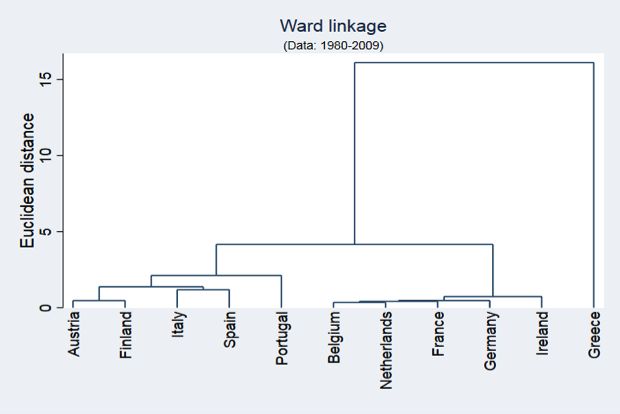
CEPII Working Paper                             Heterogeneity within the euro area: New insights into an old story

low interest rates and credit boom paved the way to the sovereign debt crisis in several
Southern member states. As currency misalignments as well as imbalances are especially
harmful in a monetary union, we consider an analysis that emphasizes how the exchange
rates have departed from their equilibrium paths.4

2.2.    Deriving nominal equilibrium exchange rate paths

    A preliminary step in our methodology is to reconcile the real approach of the equilib-
rium exchange rates with the nominal nature of a monetary union. Another is to switch
from the multilateral approach of the equilibrium exchange rates to the fixed bilateral
parities implied by a single currency.
    Regarding the transition from real to nominal, on one side, equilibrium exchange rates
are generally defined in real terms; this is also true for currency misalignments that mea-
sure the gap between the observed exchange rates and their equilibrium levels. On the
other side, a monetary union only deals with nominal parities, by fixing them irreversibly
between members, but this does not prevent the real exchange rates to evolve differently
across countries along with the relative prices. Regarding the multilateral versus bilat-
eral approach, the equilibrium exchange rate is generally assessed towards a whole set
of trade partners, whereas the monetary union defined fixed bilateral parities between
member countries.
    To sum up, we have to convert our multilateral real equilibrium exchange rates into
nominal bilateral parities. Various methods exist to deal with this issue. For example,
Alberola et al. (1999) propose a framework that allows determining nominal equilibrium
exchange rates that are consistent at the global level. Their approach consists in in-
verting the weighted matrix of effective equilibrium exchange rates to deduce bilateral
equilibrium values. However, as only (N − 1) bilateral exchange rates can be derived
from N effective rates, one currency—corresponding to the chosen numeraire—has to
be discarded. This amounts to assuming that the misalignment of the selected currency
(the rest of the world) is the mirror image of the misalignment of all other currencies.
Instead of imposing such assumption, we adopt here another approach in which nomi-
nal exchange rates that are consistent with minimized currency misalignments follow an
equilibrium path independent of each other.
4
  Couharde et al. (2013) have also developed an approach based on the use of equilibrium exchange
rates to assess the sustainability of the CFA zone; a sustainable currency area being defined as a zone in
which real exchange rates do not deviate persistently from their equilibrium paths. Similarly, Coulibaly and
Gnimassoun (2013) fall into this strand of the literature by addressing the optimality of monetary unions
in West Africa through the analysis of exchange rate misalignments.

                                                         7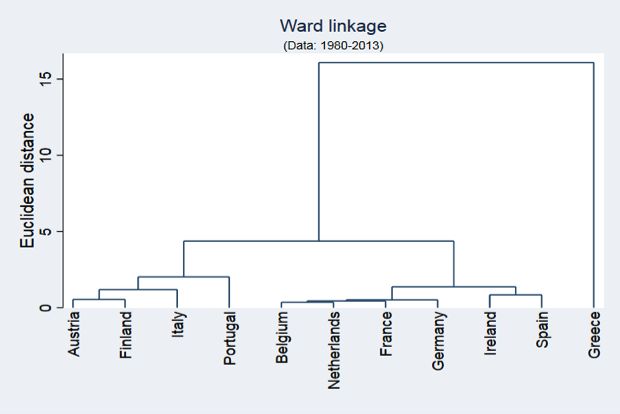
CEPII Working Paper                                    Heterogeneity within the euro area: New insights into an old story

           By definition, the real effective exchange rate of country i , REERi,t , is calculated
       as the weighted average of country i ’s real bilateral exchange rates against each of its
       N trading partners j:
                                                                       N
                                                                                      w
                                                                       Y
                                                       REERi,t =             RERij,tij,t                                 (1)
                                                                       j=1

                                                Pi,t
       where RERij,t = NERij,t ×                Pj,t    is an index of the real bilateral exchange rate of the
       country i ’s currency vis-à-vis the currency of the trading partner j in period t. NERij,t is
       the index of the nominal bilateral exchange rate between the currency of country i and
       the currency of its trade partner j in period t (number of units of currency j per currency
       i ), and Pi,t (resp. Pj,t ) stands for the price index of country i (resp. j). N denotes
       the number of trade partners, and wij,t stands is for country i ’s the trade-based weights
       associated to the for all its partners j. Note that an increase in REERi,t and NERij,t
       denotes an appreciation of currency i .

           The definition of the real effective exchange rate thus becomes:

                                         N                                                    N
                                         Y               w              Pi,t                  Y           w
                       REERi,t =               NERij,tij,t × QN                           =         NERij,tij,t × φi,t   (2)
                                         j=1                         j=1 (Pj,t   )wij,t       j=1

                          Pi,t
       with φi,t =    QN         wij,t
                       j=1 j,t )
                          (P

       Given the observed domestic and foreign price indexes and the trade-based weights,
       the equilibrium real effective exchange rate (REERi,t
                                                         ∗
                                                             ) can be written in terms of the
       equilibrium nominal bilateral exchange rate (NERi,t
                                                       ∗
                                                           ):

                                                               N
                                                               Y
                                              ∗
                                          REERi,t            =       ∗
                                                                 (NERij,t )wij,t × φi,t                                  (3)
                                                               j=1

               QN
       where             ∗
                 j=1 (NERij,t )
                               wij,t           ∗
                                         = NEERi,t is the equilibrium nominal effective exchange rate.

           We express the equilibrium bilateral nominal exchange rate (NERt∗ ) of each currency
       relative to a numeraire currency. To this end, we use the no-arbitrage property on the
       foreign exchange market that makes all the cross rates consistent, namely: NERij,t =

                                                                8
CEPII Working Paper Heterogeneity within the euro area: New insights into an old story
NERi,t
NERj,t , where NERi,t denotes the exchange rate of country i against the numeraire. We
choose the Special Drawing Rights (SDR) as the numeraire, as in Housklova and Osbat
(2009) for instance. Frankel and Wei (2008) advocated for this choice of numeraire
because monetary authorities generally do not monitor their exchange rate towards a
single currency, but have rather to focus on several key currencies. Other authors use
the dollar, the Swiss franc or several numeraires (Frankel and Wei, 1994; Bénassy-
Quéré, 1999), although this choice generally does not affect their results. Although in a
bilateral set-up the choice of the numeraire will not qualitatively affect the estimates, the
derivation of bilateral misalignments from effective misalignments leads to assessments
that are affected by the effective misalignment of the numeraire currency at all points in
time (Housklova and Osbat, 2009). The introduction of the SDR avoids this problem.
Furthermore, the use of the SDR allows us (i ) to define the value of each currency
independently of the others, and, in turn, (ii ) to derive an equilibrium exchange rate
path specific to each country. Recalling that the equilibrium exchange rate of country i
is independent from country j’s exchange rate level, Equation (3) can thus be rewritten
as follows:
N wij,t
Y 1
∗
REERi,t = ∗
SiSDR,t × × φi,t (4)
j=1
SjSDR,t
where SiSDR,t
∗
is the equilibrium nominal exchange rate of the currency of country i vis-à-
vis the SDR and SjSDR,t denotes the nominal exchange rate of the currency of country
j vis-à-vis the SDR.
Equation (4) can be rewritten as:
1 1
∗
REERi,t ∗
= SiSDR,t × QN wij,t
∗
× φi,t = SiSDR,t × × φi,t (5)
j=1 SjSDR,t
Ωi,t
QN w
where Ωi,t = j=1
ij,t
SjSDR,t corresponds to the weighted average of the nominal exchange
rate of the N trade partners vis-à-vis the SDR.
The equilibrium value of the currency of country i vis-à-vis the SDR that minimizes
9CEPII Working Paper Heterogeneity within the euro area: New insights into an old story
currency misalignments (i.e., that equalizes REERi,t and REERi,t
∗
) is then given by:
Ωi,t
∗
SiSDR,t ∗
= REERi,t × (6)
φi,t
The time series of this equilibrium bilateral exchange rate allows us determining the
paths of equilibrium parities SiSDR,t
∗
against the numeraire.
2.3. Assessing equilibrium exchange rates
There are three approaches of equilibrium real exchange rates: (i ) the fundamental
equilibrium exchange rate (FEER; Williamson, 1994) approach also referred to as the
macroeconomic approach, (ii ) the external sustainability approach, and (ii i ) the behav-
ioral equilibrium exchange rate (BEER; Clark and MacDonald, 1998) approach. In the
FEER framework, the equilibrium real exchange rate corresponds to the exchange rate
level that allows the current account—projected over the medium term at prevailing
exchange rates—to converge towards an estimated equilibrium current account, or a
current account target. In the external sustainability approach, the equilibrium exchange
rate aims at stabilizing the ratio of net foreign assets (NFA) to GDP at an appropriate
level. These two approaches share a common drawback since they require defining the
long-run equilibrium paths of economies. This exercise involves making assumptions on
the long-run values of the economic fundamentals (such as current account norms in
the FEER approach, and the appropriate ratio of NFA to GDP), which may be viewed
as quite arbitrary. On the contrary, the BEER approach directly estimates an equilibrium
real exchange as a function of medium- to long-term fundamentals, taking into account
both internal and external balances without any ad hoc judgments. In this paper, we rely
on such BEER framework for these reasons.
We consider the stock-flow model of exchange rate determination in the long run
originally proposed by Faruqee (1995)—followed by Alberola et al. (1999) and Alberola
(2003)—which is particularly suitable for describing advanced economies. This model
emphasizes the net foreign asset position and the relative sectoral productivity (i.e.,
the Balassa-Samuelson effect) as important drivers of the real effective exchange rate.
Following Clark and MacDonald (1998) among others, we augment this benchmark spec-
ification by including the terms of trade as an additional fundamental variable to account
for real shocks.5 These fundamentals are particularly relevant for the euro-area countries
5
For the sake of robustness, we have also estimated a simpler specification including only productivity
differential and net foreign asset position as determinants of real exchange rates; the results remain similar
10CEPII Working Paper Heterogeneity within the euro area: New insights into an old story
as they fairly reflect the main sources of macroeconomic imbalances within the EMU
that have been stressed: inflation rate differentials exceeding what could be explained by
Balassa-Samuelson effects (Belke and Dreger, 2013), presence of large stock imbalances
(Lane, 2013), and finally real shocks paving the way for asymmetric shocks. The full
specification of our model is then the following:
r eeri,t = µi + β1 r pr odi,t + β2 nf ai,t + β3 toti,t + εi,t (7)
where r eeri,t is the real effective exchange rate (in logarithm), r pr odi,t stands for the
relative productivity (in logarithm), nf ai,t is the net foreign asset position (as share of
GDP), and toti,t denotes relative terms of trade, expressed in logarithm. µi are the
country-fixed effects and εi,t is an error term. A positive relationship between the real
effective exchange rate and each of the fundamentals is expected. Once the coefficients
estimated, the equilibrium real exchange rate r eeri,t
∗
will be calculated as the fitted value
of r eeri,t in Equation (7). Corresponding currency misalignments, Mi si,t , are then given
by: Mi si,t = r eeri,t − r eeri,t
∗
.
2.4. Data and results
Our panel consists of the following eleven eurozone countries: Austria, Belgium,
Finland, France, Germany, Ireland, Italy, the Netherlands, Portugal and Spain; i.e., the
founding members of the euro area in 1999 plus Greece which joined the union in 2001.6
The data are annual and cover the 1980-2016 period.7 To assess equilibrium real ex-
change rates, we collect real exchange rate indexes from the EQCHANGE database
provided by the CEPII.8 These indexes correspond to the real effective exchange rates
vis-à-vis 186 trading partners computed using time-varying weights representative of
trade flows (5-year windows).9 These REER indexes are defined so that an increase
corresponds to a real appreciation of the domestic currency. We use the same trade
partners and weights for the calculation of the relative productivity, proxied here by the
relative real GDP per capita (in PPP terms).10 The net foreign asset positions are
and are available upon request.
6
Luxembourg and the other countries are excluded due to data availability issues during the 1980s and
1990s.
7
See Table A.1 in Appendix A for details regarding the data.
8
http://www.cepii.fr/CEPII/fr/bdd_modele/presentation.asp?id=34.
9
The use of time-varying weights is important to move closer to the reality by capturing trade dynamics.
See Couharde et al. (2018) for details regarding the EQCHANGE database.
10
Due to the lack of sectoral data on output and employment for traded and non-traded goods sectors,
most empirical studies test the Balassa-Samuelson hypothesis by relating the real exchange rate to the
11CEPII Working Paper Heterogeneity within the euro area: New insights into an old story
extracted from the Lane and Milesi-Ferretti (2007) database (extended to 2014) and
updated using information on national current accounts provided by the IMF databases
(International Financial Statistics and World Economic Outlook). The terms of trade
series are taken from the World Bank’s WDI (World Development Indicators) database.
We rely on the cross-sectionally augmented pooled mean group procedure (CPMG;
see Pesaran, 2006; Binder and Offermanns, 2007; De V. Cavalcanti et al., 2015) to
estimate the long-run relationship between the REER and its fundamentals, described by
Equation (7). This method has the advantage to provide consistent estimates of a long-
run relationship in presence of cross-sectional dependencies. Indeed, CPMG augments
the pooled mean group procedure (PMG; see Pesaran et al., 1999) with cross-sectional
averages of the variables, therefore accounting for unobservable common factors. Fur-
thermore, the CPMG procedure, compared to other long-run estimation methods (e.g.
dynamic OLS, fully-modified OLS), better accounts for potential heterogeneity between
countries as it allows short-run dynamics heterogeneity for each member of the panel.11
The CPMG procedure appears therefore as the most adequate to capture not only in-
terdependencies between countries, but also each country particularities (e.g. resilience
to shocks). However, as a condition for the efficiency of the CPMG estimator is homo-
geneity of the long-run parameters across countries, we also rely on the cross-sectionally
augmented mean group estimator (CMG) and test the long-run slope homogeneity hy-
pothesis.12
Table A.2 in Appendix A presents the CPMG and CMG estimates, as well as the
Hausman test statistic examining panel heterogeneity. According to the test statistic,
the long-run homogeneity restriction is not rejected for individual parameters and jointly
in all regressions. We therefore focus on the CPMG estimates. Considering the whole
period, results reported in Table A.2 appear consistent with the theory since the coeffi-
cients have the expected signs. Indeed, the real effective exchange rate appreciates in
the long run with the increase in the relative real GDP per capita (in PPP terms), the
improvement in the net foreign asset position and in the terms of trade.
The fitted values of real effective exchange rates given by the estimation of Equa-
real GDP per capita (in PPP terms) differential which is a common measure for productivity. We follow
here the same approach.
11
Further note that all the mentioned procedures impose long-run slope homogeneity but, in the case of
the CPMG procedure, this hypothesis can be tested (Hausman-test type).
12
The CMG procedure provides consistent estimates of the averages of long-run coefficients, although
they are inefficient if homogeneity is present. Under long-run slope homogeneity, the CPMG estimates are
consistent and efficient (De V. Cavalcanti et al., 2015).
12CEPII Working Paper Heterogeneity within the euro area: New insights into an old story
tion (7) provide the equilibrium real exchange rates.13 Then we calculate the nominal
equilibrium rates against the SDR (SiSDR,t
∗
) from Equation (6). To this end, we deflate
the equilibrium real effective exchange rate series by the weighted relative prices (Φi,t )
that are used for the computation of REER indexes in the EQCHANGE database.14
Finally, equilibrium real exchange rates are adjusted for movements in the nominal bilat-
eral exchange rates of trading partners vis-à-vis the SDR (variable Ωi,t constructed as a
weighted average).15
3. Evaluating the distance between euro-area countries: a cluster analysis
The purpose of this section is (i ) to identify relatively homogeneous groups of euro-
members based on their respective equilibrium exchange rate path, and (ii ) to examine
whether the subsequent partition of the euro area has evolved over time, specifically
since the launch of the single currency. To assess the size of dissimilarities across euro-
area countries, we implement a cluster analysis, based on the hierarchical ascendant
classification (HAC). This method allows us partitioning the eurozone into relatively ho-
mogeneous groups of countries without imposing any reference group or leading country
as in business cycle synchronization analyses. Moreover, it provides further information
on the level of heterogeneity in the euro area, by evidencing interrelationships within and
between the different groups of economies.
3.1. The method
The HAC procedure begins by estimating the dissimilarities between any pair of objects
(here the dissimilarities between the optimal exchange rate paths for any pair of euro-
area countries) using an appropriate metric (i.e., a measure of distance between pairs
of objects). Here we use the standard Euclidian distance.16 Let Xi,t be the optimal
exchange rate for country i at period t (t = T1 , . . . , TN ), the dissimilarity coefficient
defined by the Euclidean distance between the optimal exchange rate of country i and
13
Figure A.1 in Appendix A displays the calculated real effective exchange rates and estimated equilibrium
real exchange rates. Corresponding misalignments are reported in Figure A.2.
14
Weighted relative prices are computed as a geometric average of the ratios of the Consumer Price Index
(CPI) of a country to the CPI indexes of its main trade partners. The CPI series are from the IMF and
OECD databases (see Couharde et al., 2018).
15
Nominal bilateral exchange rates vis-à-vis the SDR are extracted from the IMF database.
16
While other measures exist (Squared Euclidean distance, Manhattan distance . . . ), the Euclidian distance
is the most common metric. Since we are working in a continuous space where all dimensions are properly
scaled and relevant (due to the numeraire currency), the Euclidean distance is the best choice for the
distance function. In addition, it does not suffer from sensitivity to outliers and is a real metric.
13CEPII Working Paper Heterogeneity within the euro area: New insights into an old story
country j is: v
u TN
uX 2
d(Xi , Xj ) = ||Xi , Xj || = t Xi,t − Xj,t (8)
t=T1
where d(Xi , Xj ) or ||Xi , Xj || denotes the Euclidean distance between Xi and Xj .
Using distance information, pairs of objects are grouped into clusters that are further
linked to other objects to create bigger clusters. The algorithm stops when all the objects
are linked. This agglomeration is realized using another metric that measures the distance
between two clusters and therefore determines the borders of the homogeneous groups.
We adopt here the following four agglomerative methods: (i ) Ward’s linkage, (ii )
single-linkage, (ii i ) complete-linkage, and (iv ) average-linkage. Let A and B be two
clusters with, respectively, nA and nB as the number of objects, and A and B as the
centroids. The Ward’s method, which is the most commonly used procedure, consists
in joining two clusters that result in the minimum increase in the sum of squared errors
(so the loss of within-cluster inertia is minimum). The within-cluster sum of squares is
defined as the sum of the squares of the distances between all objects in the cluster and
the centroid of the cluster. The Ward’s method relies on the distance dW between the
centroids of the two clusters X A and X B :
2nA nB 2
dW (A, B) = k XA − XBk (9)
(nA + nB )
The single-linkage, also called “nearest neighbor”, considers the smallest distance dS
between objects in the two clusters. On the contrary, the complete-linkage or “furthest
neighbor”, as it name suggests, concentrates on the largest distance dC between objects
in two clusters. Finally, the average-linkage method uses the average distance dA between
all pairs of objects in any two clusters.17 These inter-cluster distances are expressed as
follows:
(10)
dS (A, B) = mi n d XAi , XBj
(11)
dC (A, B) = max d XAi , XBj
nA XnB
1 X
(12)
dA (A, B) = d XAi , XBj
nA nB i=1 j=1
17
For more details regarding these measures, see Kaufman and Rousseeuw (1990).
14CEPII Working Paper Heterogeneity within the euro area: New insights into an old story
where i = 1, . . . , nA (resp. j = 1, . . . , nB ) designates the i th (resp. j th ) object in cluster
A (resp. B).
We use the HAC analysis to measure the distance between the euro-area countries
regarding the path of their equilibrium exchange rates. First, we consider the period
before the monetary union 1980-1998. Then, we study how the clustering of countries
has evolved over time. To do so, we perform the same cluster analysis over different
time periods in order to track structural changes. This investigation aims at capturing
any change in dissimilarities across the euro area. On the whole, we retain three periods
all starting in 1980: (i ) before the monetary union: 1980-1998; (ii ) before the global
financial crisis: 1980-2006; and (ii i ) the whole period 1980-2016.
3.2. Cluster analysis before the launch of the euro
The groups identified by applying the HAC analysis before the launch of the euro are
shown in the four dendrograms reported in Figure 1. These "cluster trees" indicate the
order in which successive aggregations were made (and therefore the optimal groupings).
The vertical axis of the dendrograms represents the distance or dissimilarity between the
objects (i.e., the countries’ equilibrium exchange rate paths), while the horizontal axis
displays the different countries. The dissimilarity measures are captured by the heights
of the links.
As can be seen, the four different methods release consistent information regarding
dissimilarities in exchange rate paths across the eurozone members. From these dendro-
grams, we clearly identify two clusters of countries (two branches that occur at about
the same vertical distance). A first cluster can be identified as the “core countries”, it
includes Germany, Belgium, the Netherlands, France and Ireland. A second group of ho-
mogeneous countries is made of Austria, Spain, Italy and Finland. Portugal and Greece
are fused separately at much higher distances compared to the other countries and can
be considered as two outliers.18
The division of the euro area into several groups of countries is quite in line with
the existing literature while the composition of the core group may differ depending on
research undertaken.19 For instance, applying clustering techniques to a set of OCA vari-
18
This can be confirmed by the dissimilarity matrices reported in Appendix C for the 1980-1998 (Table
C.1) and 1980-2016 (Table C.2) periods: as shown, Greece and, to a lesser extent, Portugal are the two
countries exhibiting the highest values.
19
Part of these differences can be related to the definition of membership of the core. While the approach
suggested by Bayoumi and Eichengreen (1993) defines core countries as those whose aggregate supply
and demand shocks are relatively highly correlated with Germany, the clustering approach separates the
15CEPII Working Paper Heterogeneity within the euro area: New insights into an old story
ables, Artis and Zhang (2001) also find evidence in support of three groups of countries:
those belonging to the core (Germany, France, Austria, Belgium and the Netherlands),
those part of a Northern periphery (Denmark, Ireland, the UK, Switzerland, Sweden,
Norway and Finland) and those belonging to a Southern periphery (Spain, Italy, Por-
tugal and Greece). Also relying on OCA theory but using a modified Blanchard-Quah
decomposition within the aggregate supply – aggregate demand setup, Bayoumi and
Eichengreen (1993) identify (i) a core composed of Germany, France, Belgium and the
Netherlands, and (ii) a periphery including Greece, Ireland, Italy, Portugal and Spain.
Three sets of countries are also obtained by Bayoumi and Eichengreen (1997), distin-
guishing the economies in terms of readiness for EMU: Germany, Austria, Belgium and
the Netherlands which exhibit a high level of readiness; Finland and France which ex-
perienced little convergence; and Italy, Greece, Portugal and Spain which are gradually
converging.
Looking back on the debates at the introduction of the euro, our results thus confirm
that dissimilarities across the euro area candidates persisted until the eve of the EMU.
If we restrict our sample to the countries that adopted the euro in 1999 (i.e., excluding
Greece), two groups of countries are clearly identified, with Portugal as an outlier. From
this point of view, our results are consistent with the findings of the OCA literature
that counselled against the pursuit of further and deeper monetary integration within
Europe at that time. The partition of the euro area into different groups of relatively
homogenous countries called into question (i ) the effectiveness of Maastricht criteria in
making these countries converge before the launch of the euro, and (ii ) the desirability
of a unique monetary policy for all the economies composing these groups. Our results
also reflect the argument advanced by Eichengreen (1993) and Feldstein (1997) that
much of the driving force for monetary union was political, as in economic terms the
eurozone project would have been postponed or designed differently to allow for some
flexibilities between the core and the periphery.
3.3. The evolution in the groupings of countries
So far, our findings cannot refute the argument that dissimilarities across the potential
eurozone member countries were due to insufficient financial integration and would be
swept off by monetary union. We now extend our analysis by including the period after
most similar countries into several clusters, without assuming a representative core country. In this latter
approach, core countries are then defined as those that are theoretically suitable for a common currency,
i.e., those forming the most homogeneous group.
16CEPII Working Paper Heterogeneity within the euro area: New insights into an old story
the launch of the single currency in order to analyze the evolution of cluster memberships
over time. The corresponding results are displayed in Figure 2.20 The configuration of the
eurozone shares the same features as before, with a set of core countries and a second
group of economies. These two groups are fused at the same distance, suggesting
that the monetary union has not reduced dissimilarities between these two clusters of
countries. The peripheral countries seem also more fragmented in sub-groupings. In
particular, Italy now exhibits slightly distinct features from the other members, and is
depicted as a singleton inside the peripheral group. This is also the case for Portugal,
which is linked to the peripheral set in a single element group. Greece still appears as
an outlier, neither linked to core nor to peripheral members. It has even become more
distinct from the other countries over time as the distance to the other clusters has
increased. These latter results are in line with those of Wortmann and Stahl (2016) and
Ahlborn and Wortmann (2018) who apply different cluster algorithms respectively to the
Macroeconomic Imbalance Procedure (MIP) indicators and to output gap series. They
also find evidence in support of a strengthening over time of the core–periphery structure
of the euro area.
20
To save space, we only report the results obtained with the Ward method. The three other approaches
lead to similar results, which are available upon request to the authors.
17CEPII Working Paper Heterogeneity within the euro area: New insights into an old story
Figure 1 — HAC analysis results (1980-1998)
18CEPII Working Paper Heterogeneity within the euro area: New insights into an old story
Figure 2 — Recursive HAC analysis results
19CEPII Working Paper Heterogeneity within the euro area: New insights into an old story
On the whole, these findings suggest that the configuration of the eurozone since the
launch of the single currency has become more fragmented; dissimilarities between groups
of countries have augmented. The peripheral countries that are aggregated together
exhibit some increased distinct features. The comparison between the graphs before and
after the 2007-08 collapse shows that the adjustment that followed the financial crisis
has not changed the deal between countries. The clusters have not been brought closer
despite all the steps that have been taken to counter imbalances.
4. Identification of heterogeneous patterns: a factor analysis
Apart from the partition of countries by itself, it is also interesting to analyze which
variables have mostly explained the formation of such clusters. For this purpose, we now
develop a factor analysis in order (i ) to identify the common features shared by euro-
area countries belonging to the same group, and (ii ) to check if the results are similar
to those issued from the cluster analysis. Accordingly, we collect data on several key
variables that are more prone to reflect macroeconomic imbalances. Then, we perform a
factor analysis to identify the structural economic differences between the EMU members
emphasized by the cluster analysis.
4.1. Method and selected indicators
We use factor analysis to select the main relevant indicators, i.e., the variables that
underlie the formation of clusters. Specifically, being a multivariate explorative analysis
tool, factor analysis gathers together several variables with similar patterns and containing
most of the information into a few interpretable unobserved (underlying) variables, called
factors. Thus, as a technique of data reduction, the aim is to reduce the dimension of the
observations by grouping p observed variables into a lower number, say k, of factors. To
this end, the p variables are modeled as a linear combination of the potential factors (i.e.,
latent unobserved variables that are reflected in the behavior of the observed variables)
plus an error term. In doing so, factor analysis is a useful tool to detect the structure
of the relationships between the variables. Specifically, let us assume we have a set
of p observable random variables (Y1 , . . . , Yp ). From these p observed variables, factor
analysis aims at identifying k common factors which linearly reconstruct the original
variables as follows:
Yij = Zi1 γ1j + Zi2 γ2j + ... + Zik γkj + uij (13)
20CEPII Working Paper Heterogeneity within the euro area: New insights into an old story
where Yij is the value of the i th observation of the j th variable (j = 1, . . . , p), Zil is the
value of the i th observation of the l th common factor (l = 1, . . . , k), the coefficients γlj
denote the factor loadings (l = 1, . . . , k), and the error term uij is the unique factor of
the j th variable.
The selection of indicators must meet the need for both comprehensiveness and parsi-
mony in order to set out clear factors that can be easily interpreted. We select indicators
among a set of fundamental variables often linked to the formation of imbalances within
the euro area. This set includes the current account balance, consumer price, inflation,
public debt, GDP per capita, real growth, output gap, unemployment rate and unit labor
cost, to which we add the currency misalignments that we have calculated. Table A.1
in the appendix details the source of these series. This set of variables is large enough
to account for the usual OCA criteria as well as the economies’ internal and external
balances and their dynamics. For example, inflation obviously accounts for price stabil-
ity and debt-to-GDP ratios measure the soundness and sustainability of public finances:
these two variables, as well as unemployment rates are able to gauge the internal equilib-
rium of the economies.21 Regarding the external balance, the current account-to-GDP
ratio encompasses various key determinants according to the usual medium to long-term
specifications such as net foreign asset position, fiscal position, output gap, population
growth rate, dependency ratio, openness, etc. (see e.g. Chinn and Prasad, 2003; Gru-
ber and Kamin, 2007; Cheung et al., 2010); it has thus the advantage of parsimony by
synthetizing them in a sole series.
The selected variables should also meet considerations/rules regarding the function-
ing of the euro area, although rules much changed over the long period 1980-2016 that
we consider. For example the Maastricht criteria were important before the monetary
union, then the stability and growth pact (SGP) and the “six-pack” legislation, including
the MIP, in the aftermath of the 2008 crisis.22 We therefore take stock of the macroeco-
nomic imbalance procedure (MIP) that the European Commission has been using since
2011 in order to deal with imbalances in the member countries. Most of the 14 headline
21
Beyond all the technical aspects and rules regarding the limits of the variables mainly defined by the
Maastricht Treaty (i.e., an inflation rate that should be lower than a reference value—defined as the average
of the inflation rates in the 3 eurozone member states with the lowest inflation plus 1.5 percentage points;
a debt ratio that should not exceed 60%) or SGP rules (the unemployment three-year moving average
should be lower than 10%), factor analysis ignores such rigidity in the criteria and simply maps out the
countries on the basis of their proximity regarding the variable levels, thus potentially underlining clusters
of countries.
22
It should be noted that for the sake of consistency and uniformity of the analysis, the selection of the
variables must satisfy both ex ante prospective and ex post evaluation exercises. This explains why we did
not restrict the analysis to the sole convergence criteria.
21CEPII Working Paper Heterogeneity within the euro area: New insights into an old story
indicators that are monitored in this procedure are taken into account in our analysis.
Indeed, both the 3-year moving average of the current account (% of GDP) and the
net international investment position (% of GDP) indicators are considered either (i )
directly through the current account, or (ii ) through currency misalignments thanks to
the net foreign asset position. As well, the 3-year percentage change of the real effective
exchange rate is also accounted for via the currency misalignments.23
The detailed results of the factor analysis are presented in Appendix B.2; Table
B.1 giving some descriptive statistics on the variables. Specifically, Tables B.2.1.1 and
B.2.1.2 (respectively B.2.2.1 and B.2.2.2) are related to the results of the unrotated
analysis for the 1980-1998 (respectively 1999-2016) period, the other tables in Appendix
B.2 concerning the rotated analysis.24 Each variable is assigned to the factor in which it
has the highest loading. Once (i ) variables have been assigned to the common factors
and (i i ) the factors and their loadings have been estimated (right-hand side of Equation
(13)), the factors must be interpreted. To this end, the factor loadings have to be
examined.
4.2. Factor analysis before monetary union
Let us start with the pre-EMU, 1980-1998 period. As shown in Table B.2.1.1 in
Appendix B, only the first three factors are retained as the eigenvalues associated with
the other factors are negative. The first two factors are the most meaningful, explaining
the major part (around 75%) of the total variance (Table B.2.1.3). Table B.2.1.4 shows
that the first factor (Factor 1 ) has a high positive correlation with inflation and the
debt-to-GDP ratio, and a high negative correlation with the current account balance.
Factor 1 thus principally opposes (i ) on the left side, the current account balance and,
(i i ) on the right side, the debt-to-GDP ratio and inflation. Accordingly, Factor 1 may be
interpreted as the “Finance/Wealth axis” or reflecting the “Financial position”: on the left
side, countries with good/sustainable foreign position; on the right side, countries facing
external imbalances characterized by a high inflation rate and a high debt-to-GDP ratio,
which result in current account deficits. The second factor, Factor 2, correlates strongly
23
Furthermore, we consider the country total debt (government plus private sector) while in the MIP
scoreboard a distinction is made regarding the debt indicators. By the same token, we use the total
economy unemployment rate instead of the different types/horizons of unemployment.
24
Recall that factor loadings could be rotated to make easier the interpretation of the factors. Indeed,
rotation consists in expressing the factors so that loadings on a quite low number of variables are as large as
possible, while being as small as possible for the remaining variables. Here, we retain the usual orthogonal
varimax rotation (Kaiser, 1958) which maximizes the variance of the squared loadings within factors.
22CEPII Working Paper Heterogeneity within the euro area: New insights into an old story
and positively with the indicators for unemployment and misalignments, and negatively
with economic growth. Factor 2 may thus appropriately reflect internal imbalances
(Table B.2.1.4).
Regarding methodological aspects, our results are satisfying as shown by the low
values of uniqueness in Table B.2.1.4. Indeed, recall that uniqueness measures the
percentage of variance for the considered variable that is not explained by the common
factors. Uniqueness could represent measurement error, which is likely if it takes a
high value, typically larger than 0.6. The values we obtain being quite low (except for
inflation), our retained variables are well explained by the identified factors.
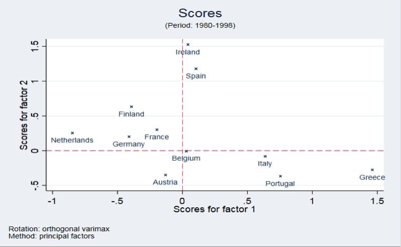
The results regarding the first two factors are synthesized in Figure 3. Specifically,
the top chart, i.e., the factor loadings plot, displays the position of each variable in the
Factor 1 -Factor 2 plane. Its aim is to identify clusters of variables with similar loadings.
The bottom chart (“Scores”) of Figure 3 displays the score of individual countries on
each factor, the values being provided in Table B.2.1.6. The closer the country is to a
variable, the more important is the score of the country regarding this variable.
An interesting observation, which is in line with the results of the cluster analysis, is
that Greece and, to a lesser extent, Portugal score very high with respect to external
imbalances. Their position appears far from that of any other country (except Italy).
With the HAC analysis, Greece and Portugal were viewed as outliers among the eurozone
countries in the sense that they were the last countries that merged into the final cluster
that included all other members. This is reflected by their extreme position in the scores
plot, (i ) close to Debt and Inflation suggesting the highest debt and inflation levels—on
average—, and (ii ) far away from the other variables (as the current account position),
reflecting recurrent current account deficits. The positions of Greece and Portugal as
outliers are therefore confirmed by their poor performance reflected in high financing
requirements before the launch of euro area.25
Another interesting finding which also corroborates the results of the cluster analysis is
that some core countries score rather low on the factor of external imbalances: France,
Germany, the Netherlands and Belgium. As showed by the bottom chart of Figure
3, these countries form a cluster at the left-center of the scores plot, indicating that
they had low inflation rates and debt-to-GDP ratios before the EMU, which resulted in
lower current imbalances and/or current surpluses. Other countries either score high
on the factor of external imbalances, such as Italy, or score low on this factor, but
25
The bad performance of Greece is confirmed by the highest score displayed by this country when con-
sidering the third factor (see Table B.2.1.6).
23CEPII Working Paper Heterogeneity within the euro area: New insights into an old story
Figure 3 — Factor analysis results (1980-1998)
at the expense of higher internal imbalances, as Spain and Finland. Although Austria
appears close to the core group, Factor 2 —which displays a strong correlation with
misalignments—makes this country apart from the group composed by France, Germany,
the Netherlands and Belgium, as highlighted by the cluster analysis.26 Only the position
of Ireland gives a picture that is less clear-cut than the one delivered by the cluster
analysis. Indeed, whereas Ireland is merged into the core group when the clustering
method is used, its high unemployment rate makes it move away from the core in the
26
It should be noted that the position of Austria is not straightforward as this country is found to be in
the core group over the 1980-1998 period when we use the k-means procedure as an alternative clustering
method (see Appendix D).
24CEPII Working Paper Heterogeneity within the euro area: New insights into an old story
factor analysis. This gap is partly explained by the highest—negative—score regarding
the third factor displayed by Ireland. As this third factor is not represented in Figure 3,
this may affect the global pattern. Despite these facts, its position issued from the factor
analysis remains compatible with our previous findings. Indeed, the factor analysis being
performed using data on the total unemployment rate, its result simply highlights that
Ireland was one of the countries exhibiting the highest unemployment rate before the
monetary union. Meanwhile, Ireland also had a quite high—estimated—NAIRU (Non-
Accelerating Inflation Rate of Unemployment) which makes the aforementioned rate of
unemployment sustainable, i.e., reflecting a situation of near internal balance.
Overall, this first factor analysis proves to be very informative and comes in support to
the findings of the HAC analysis. Indeed, both approaches suggest that Belgium, France,
Germany, the Netherlands, and Ireland form the core group. While the picture for the
first four aforementioned countries is clear-cut from both the cluster and factor analyses,
the inclusion of Ireland—indicated by the HAC approach—is also found relevant by the
factor analysis, except for the unemployment figure. The other economies appear quite
dissimilar; with persistent imbalances, the participation to the monetary union together
with these core countries would imply costs. This is particularly true for Greece and, to
a lesser extent, for Portugal.27
4.3. Factor analysis after the launch of the euro
Let us now turn to the 1999-2016 period to examine how the observed trends have
evolved since the launch of the single currency, and whether they remain consistent with
those derived from the cluster analysis.
As for the previous pre-EMU period, two principal factors explain most (about 90%) of
the total variance (Tables B.2.2.1 and B.2.2.3), while reflecting different patterns (Table
B.2.2.4). The first factor may now be interpreted as reflecting “virtuous countries”: this
axis opposes the debt-to-GDP ratio on the left side, and growth on the right side. For
its part, Factor 2 can be seen as ranking countries facing macroeconomic imbalances:
it displays negative and important correlation with the current account balance, and is
positively correlated with unemployment and inflation. Hence, the higher the country’s
score on this axis is, the larger its macroeconomic imbalances.28 Thus, the two principal
27
In contrast with Greece, the analysis indicates that Portugal only suffers from competitiveness problems.
This holds for Spain, but to a lesser extent.
28
Note that the third factor is principally defined by currency misalignments—while opposing them with
the current account balance. Factor 3 can thus be seen as the competitiveness factor: the higher the
overvaluations, the lower the trade performances.
25You can also read