Working Paper Series No country is an island: international cooperation and climate change
←
→
Page content transcription
If your browser does not render page correctly, please read the page content below

Working Paper Series
          Massimo Ferrari, Maria Sole Pagliari   No country is an island:
                                                 international cooperation
                                                 and climate change

                                                   No 2568/ June 2021

Disclaimer: This paper should not be reported as representing the views of the European Central Bank
(ECB). The views expressed are those of the authors and do not necessarily reflect those of the ECB.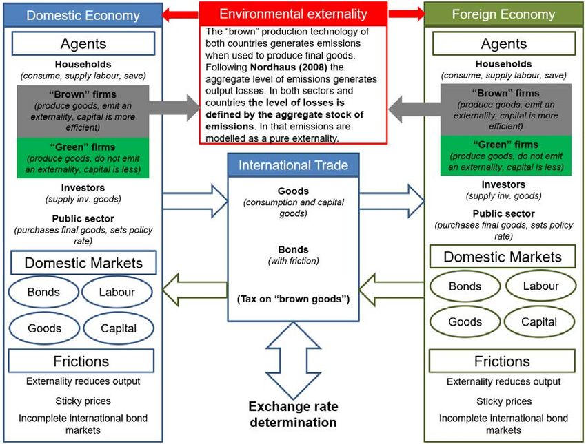
Abstract

       In this paper we explore the cross-country implications of climate-related mitigation policies.
       Specifically, we set up a two-country, two-sector (brown vs green) DSGE model with negative
       production externalities stemming from carbon-dioxide emissions. We estimate the model
       using US and euro area data and we characterize welfare-enhancing equilibria under alter-
       native containment policies. Three main policy implications emerge: i) fiscal policy should
       focus on reducing emissions by levying taxes on polluting production activities; ii) mone-
       tary policy should look through environmental objectives while standing ready to support
       the economy when the costs of the environmental transition materialize; iii) international
       cooperation is crucial to obtain a Pareto improvement under the proposed policies. We
       finally find that the objective of reducing emissions by 50%, which is compatible with the
       Paris agreement’s goal of limiting global warming to below 2 degrees Celsius with respect to
       pre-industrial levels, would not be attainable in absence of international cooperation even
       with the support of monetary policy.

       Keywords: DSGE model, open-economy macroeconomics, optimal policies, climate mod-
       elling

       JEL Codes: F42, E50, E60, F30

ECB Working Paper Series No 2568 / June 2021                                                             1
Non-technical summary

The discussion on the impact of climate change and of potential mitigation policies has gained
momentum both in academia and policy circles over the last decades. Heatwaves, floods and
natural disasters at broad are raising the awareness that the long-neglected costs of adverse
climatic events might materialize sooner than expected. Scientific studies, endorsed by interna-
tional agreements, have estimated that countries should reduce their emissions by about 50%
in order to maintain the increase in temperature below 2 degree Celsius over the next century
(IMF (2019)). Research networks involving central banks and policy institutions have been
created to discuss how to best tackle climate change and how to calibrate mitigation policies.
A recent report by the Network for the Greening of the Financial System (NGFS), organized
by 87 central banks and supervisory authorities, for example, provides a detailed analysis of
the potential impacts of climate change onto the economy and the central banking operations
(NGFS (2020)).
Despite there exist robust empirical evidences on the macroeconomic costs of higher emission
levels (Nordhaus (1994) and Hsiang et al. (2017)), there are relative few structural macro models
featuring emission externalities that can be used to analyse the trade-off of different containment
policies. Moreover, most of the existing macro-literature mainly makes use of closed-economy
frameworks with no cross-country interaction (e.g., Heutel (2012), Ferrari and Nispi Landi
(2020) and Dietrich et al. (2021)). Against this backdrop, our paper provides four new con-
tributions. First, we derive an open economy general equilibrium model where emissions and
their spillovers can be studied in a structural framework. In our setting there are two countries,
each of which produces “brown” and “green” goods. The two goods are perceived as similar
by consumers, but the production of brown goods generates a negative emission externality. In
this context, the cross-country dimension is particularly relevant because emissions produced in
once country affect also the other. As a consequence, only cooperative actions are successful in
reducing climate risk at the global level. In economic terms, this is a coordination problem, as
actions produce the maximum benefits only if taken jointly. However, profit-maximizing agents
might refrain from doing anything as they would benefit more by waiting for other agents to act.
Second, we estimate the model with US and euro area data to study how emissions patterns
across the Atlantic have changed over the last 20 years. Notably, in our framework the “social
cost” of emissions, which is given by the GDP loss due to emissions in the steady state, amounts
to around 1.2% of GDP in the US, a figure which looks more realistic and aligned to the empirical
estimates compared to other calibrated models’ predictions. Third, we compare different policies

ECB Working Paper Series No 2568 / June 2021                                                     2
that can be deployed to reduce emissions: i) a change in monetary policy objectives, whereby
the central bank pursues a double mandate of maximizing welfare and reducing emissions; ii) a
change in domestic fiscal policy, whereby fiscal authorities start to directly tax emissions; iii) a
change in trade policy,whereby one country implements tariffs targeting polluting imports from
the foreign economy. We additionally evaluate the consequences of coordinated and competitive
actions by agents. Specifically, we show that the non-cooperative equilibrium is characterized
by an insufficient level of taxation on emissions, as both countries attempt to entirely pass the
cost of emissions containment on to their respective counterpart. Therefore, only coordinated
policies can achieve the climate objective when fiscal and monetary policy interact. Notably,
the best policy mix is the one where governments focus on reducing emissions, while the central
banks intervene to reduce the welfare costs of environmental taxation.

1       Introduction

The discussion on the impact of climate change and of potential mitigation policies has gained
momentum both in academia and policy circles over the last decades. Heatwaves, floods and
natural disasters are raising the awareness that the long-neglected costs of adverse climatic
events might materialize sooner than expected. Scientific studies, endorsed by international
agreements, have estimated that countries should reduce their emissions by about 50% in order
to maintain the increase in temperature below 2 degree Celsius over the next century (IMF
(2019)). Networks among central banks and policy institutions are now discussing how to best
tackle climate change and how to calibrate mitigation policies. NGFS (2020), for example,
provides a detailed analysis of the potential impacts of climate change onto the economy.
In spite of the wide and growing empirical literature that tries to quantify the costs of climate
events and to assess the relationship across emissions, climate disasters and economic perfor-
mance, few structural models have been developed in this field1 . Such frameworks could be
anyways useful to study the implications of policies that have arguably never been implemented
before and, therefore, cannot be ascertained on the basis of past data. Among the existing
contributions on this topic, Heutel (2012) is the first to provide a structural model where emis-
sions are endogenous and affect output.2 One advantage of using structural models is that they
    1
     Notably, there are several empirical contributions that focus on the assessment of physical and transitional
climate risks in the financial sector. See, for instance, Pagliari (2021) for a study of the relationship between
climatic adverse events and banking performance in the euro area, or Allen et al. (2020) for the setup of an
analytical framework to quantify the impacts of climate policy and transition narratives on economic and financial
variables that are necessary for financial risk assessment. Finally, refer to Tol (2009) for a thorough survey of the
early theoretical macroeconomics literature on climate change.
   2
     There indeed exists a wide literature on the quantification of the cost of climatic events, for example Nordhaus
(2008). However models in the spirit of DICE or FUND have been developed to account for several sources of

ECB Working Paper Series No 2568 / June 2021                                                                       3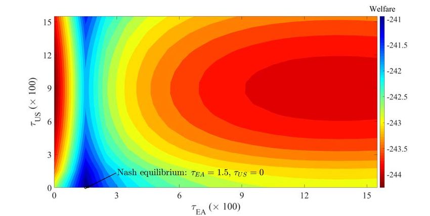
can be used to formally study optimal policy problems and identify trade-offs between different
specifications of the policies of interest. The literature on optimal policy in DSGE model is vast,
including the pioneering work of Woodford (2003) on monetary policy, but only recently these
tools have been applied to the design of climate change mitigation policies (Benmir et al. (2020),
Kotlikoff et al. (2020)). Against this backdrop, our paper provides five relevant contributions.
First, we show that there are relevant non-linearities in the relationship between carbon emis-
sions, a common measure of climate externalities, and macro variables. For example, when the
level of emissions is low there is a positive correlation between CO2 and GDP, because more
output leads to more emissions, but the emission stock is too low to generate sizeable climate
events. When the stock of CO2 is high, on the contrary, that correlation drops because more
emissions directly increase the severity of climate shocks leading to GDP losses. These results
suggest that empirical models, if anything, underestimate the real costs of climate externalities
on full sample estimations. Second, we derive an open economy general equilibrium model where
emissions and their spillovers can be studied in a structural framework. Specifically, we set up
a rich two-country two-sector model, where, on the one hand, “brown” production generates
a negative environmental externality that is detrimental to both domestic and foreign output,
while, on the other hand, “green” production does not. This cross-country dimension is crucial
in the debate on climate change, because only a fall in the global stock of emission would reduce
the likelihood of a “climatic disaster”, whereas isolated actions might result insufficient. In
economic terms, this is a coordination problem, as efforts produce the maximum benefit only
if taken jointly. However, profit-maximizing agents might refrain from doing anything as they
would benefit more by waiting for other agents to act, without bearing any direct cost.
Third, we estimate the model with US and euro area data to study how emissions patterns
across the Atlantic have changed over the last 20 years. In our framework the “social cost”
of emissions, which is given by the GDP loss due to emissions in the steady state, amounts to
around 1.2% of GDP in the US, a figure which looks more realistic and aligned to the empirical
estimates (Hsiang et al. (2017)) compared to other models’ predictions (Heutel (2012)). Fourth,
we evaluate the implementation of three alternative policies to reduce emissions: i) a change in
monetary policy objectives, whereby the central bank pursues a double mandate of maximizing
welfare and reducing emissions; ii) a change in domestic fiscal policy, whereby fiscal authorities
start to directly tax emissions; iii) a change in trade policy, whereby one country implements
tariffs targeting polluting imports from the foreign economy. We show that both monetary
policy and tariffs are not effective in reducing emissions, whereas domestic taxation can achieve
pollution and types of climatic events, but often rely on reduced-form equations for production and consumption
side of the economy, which make them less appealing than structural models for the welfare analysis of policies.

ECB Working Paper Series No 2568 / June 2021                                                                  4
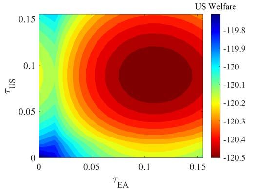
the objective. Against this background, we determine the Nash equilibrium of a game where
each country optimally sets the domestic environmental tax by responding to the opponent’s
choice. We show that such equilibrium is characterized by an insufficient level of taxation on
emissions, as both countries attempt to entirely shift the cost of emissions containment to their
respective counterpart. Therefore, only coordinated cross-country policies can attain the ap-
propriate reduction in global emissions.
We then characterize the incentive compatible policy mix, defined as the policy which reaches
the climate objective without reducing welfare in both countries, and find that it is character-
ized by a combination of fiscal and monetary policies. Notably, under such policy governments
should focus on reducing emissions while the central bank should intervene to reduce the welfare
costs of environmental policies. This joint intervention only can ensure that the climate policy
is also welfare compatible. The reason is twofold: i) the pattern of emissions is impacted more
strongly by altering the incentives of firms and inducing them to shift to a greener production.
Fiscal policy has therefore an advantage in tackling climate change compared to monetary pol-
icy, which in turn reduces fluctuations around the growth path of the economy; ii) monetary
policy plays a crucial role in stabilizing the economy once climate policies are implemented, thus
minimizing their social costs. When the environmental tax is introduced, indeed, the relative
volatility of inflation and output changes thus providing the monetary authority with the pos-
sibility to adjust its optimal reaction function, accommodate the green transition and improve
welfare.
Finally, we show that the equilibrium under international cooperation is superior to the non-
cooperative Nash equilibrium and that countries cannot credibly threaten to retaliate if their
partner deviates from environmental agreements. Our framework could then prove useful also
to address some policy issues that have become relevant in the current international debate
(NGFS (2020), McKibbin et al. (2020), Dees and Weber (2020)).

1.1       Related literature

There exists a growing literature incorporating the effects of climate change, as well as the po-
tential economic consequences of containment policies, into workhorse macroeconomic models.
These models, like ours, depart from standard DICE frameworks, such as the one of Nordhaus
(2017)3 . DICE-type models have been developed to determine the social cost of carbon (SCC),
i.e. the economic cost caused by an additional ton of carbon dioxide emissions or its equivalent,
by accounting for several sources of pollution at the same time and different dimensions of cli-
   3
       See also: The DICE-RICE model by William Nordhaus.

ECB Working Paper Series No 2568 / June 2021                                                    5
mate change such as air and sea temperatures. To preserve tractability, however, the framework
needs to rest on some simplifying assumptions: there are no assets except for investments, which
are given by the difference between output and consumption; there are no wages; prices and
interest rates are constant; the world economy is modelled as a unique block and many macroe-
conomic relations are included via reduced-form equations4 . These characteristics make the
DICE setting less appealing for optimal policy analysis as it abstracts from agents’ preferences
and expectations, trade-offs across assets and proper inter-temporal investment-consumption
decisions. Moreover, DICE models are generally simulated starting from some given initial
conditions. In other terms, they do not have a properly defined steady state which, in most
monetary and fiscal models, is the starting point for the evaluation of policies. Finally, structural
models can be estimated with standard methods whereas DICE models are typically calibrated.
For all these reasons a new generation of macro-models accounting for climate change has been
developed in recent years. Our paper fits within this growing research stream, by extending it
to a multi-country environment.
Some of the existing contributions aim at assessing the impact of fiscal policies that can be
deployed to address climate change. Heutel (2012), for instance, is the first one to include emis-
sion externalities in a DSGE model to evaluate optimal containment policies along the business
cycle. The main finding is that both quota and tax policies should be pro-cyclical, with the
tax rate and the emissions quota decreasing during recessions. Similarly, Benmir et al. (2020)
set up a theoretical model to study the optimal design of a carbon tax when environmental
factors, such as CO2 emissions, directly affect agents’ marginal utility of consumption. Using
asset pricing theory, they show that the optimal taxation policy is pro-cyclical: the carbon tax
should be increased during booms to “cool down” the economy and should be decreased to
stimulate it in recessions. Our paper differs from Benmir et al. (2020) in two respects: from
a methodological standpoint, we do not directly include emissions in the households’ utility
function; context-wise, we aim at assessing the international effects of environmental policies.
Annicchiarico and Di Dio (2015), instead, develops a New Keynesian model to study the econ-
omy under different environmental policy regimes highlighting that the optimal environmental
policy response to shocks depends on price stickiness and on the monetary policy conduct.
Other contributions focus more on the potential role of monetary policy, given that climate
change and its mitigation can have substantial repercussions on the conduct of monetary policy
along several dimensions5 . Dietrich et al. (2021), for instance, explore the so-called expectation
   4
     Another popular model for the consumption of environmental resources, the FUND model, is also based on
reduced-form equations (Waldhoff et al. (2014)).
   5
     The NGFS (2020) report outlines four crucial aspects to be considered in this regard: i) the effect on the key
macroeconomic variables that are targeted by monetary policy; ii) the effect on the main transmission channels

ECB Working Paper Series No 2568 / June 2021                                                                     6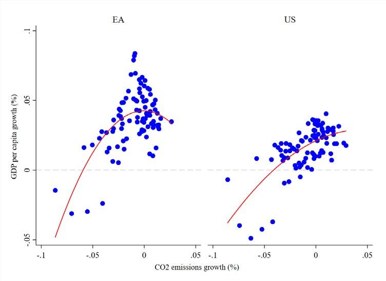
channel of climate change, whereby agents’ expectations about future climatic disasters can
negatively impact the economy today via a drop in the natural rate of interest, if the central
bank is unwilling or unable to adjust its policy in a timely manner. Given the limitations
that conventional monetary policy might face, Ferrari and Nispi Landi (2020) build a DSGE
model where the central bank can temporarily modify its balance sheet to buy bonds issued by
non-polluting firms. This Green QE is found to have limited effects in reducing the stock of
emissions and to produce positive, yet small, welfare gains.
Another aspect of the debate concerns the estimation of the real economic costs of emissions.
Tol (2009) provides an overview of the different estimates of the earliest literature, with losses in
GDP ranging from -4.8% (Nordhaus (1994)) to -0.1% (Maddison (2003)). More recently, Burke
et al. (2015) have found that climate change is expected to reshape the global economy by
reducing global economic output and possibly amplifying existing global economic inequalities,
with an estimated impact on global income of -23% by 2100. Similarly, Hsiang et al. (2017)
underscore the role of climate change in exacerbating income inequalities and estimate that,
by the late 21st century, poorest countries are projected to experience damages between 2%
and 20% of country income under the current emissions scenario. Nordhaus (2017), by revising
the estimates provided by Nordhaus (2008), quantifies the cost of CO2 emissions in the US as
being equal to 32 dollars per metric cube (3.2% of GDP). As to the effects on emerging markets,
Bombardini and Li (2020) find that a one standard deviation increase in the pollution content of
exports in China raises infant mortality by 4.1 deaths per thousand live births, which is about
23% of the standard deviation of infant mortality change. Finally Desmet et al. (2021) use a
spatial model to quantify the effects of rising sea levels that are estimated to range 0.16-0.25
p.p. of GDP in present values. In this respect, our model produces estimates of the cost of
climate externalities (in GDP terms) that are aligned to the existing empirical measures.
Another strand of research focuses on the potential consequences of policies enacted to contain
the negative effects of climate change. Brock et al. (2013), for instance, construct a computable
general equilibrium model where the degree of spatial differentiation of optimal taxes depends on
heat transportation. Keen and Kotsogiannis (2014) analyse the possibility for countries to im-
plement some form of border tax adjustments (BTAs) to countervail distortions stemming from
different carbon pricing and show that BTAs’ efficiency depends on whether climate policies are
pursued by carbon taxation or by cap-and-trade. In a similar vein, Larch and Wannera (2017)
show that the introduction of carbon tariffs in a multi-sector, two-factor gravity model reduces
welfare in most countries, with the effect being more pronounced in poorer economies. However,
as well as on the assessment of the policy space; iii) the expansion of the central banks’ analytical toolkits to
include climate-related risks; iv) the diversified impact of climate change on the different monetary regimes.

ECB Working Paper Series No 2568 / June 2021                                                                   7
they also show that carbon emissions can be shifted from these to richer countries. Nordhaus
(2015) extends the DICE framework to more countries and shows the conditions under which a
“climate club” can be established in that framework.6 In a more recent contribution, Hambel
et al. (2021) construct a DSGE model featuring a social cost of carbon, which measures the
externalities incurred into by emitting one ton of carbon dioxide to the atmosphere. Account-
ing also for the feedback effects of SCC on temperature dynamics, they show how the optimal
abatement strategy and, hence, SCC crucially depend on whether temperature has a negative
impact on either the level or the growth rate of output. Our paper also fits into this particular
literature, as it analyses the open-economy implications of containment policies. Specifically,
we focus on the risks stemming from a lack of international cooperation, thus highlighting the
importance of cross-country coordination when it comes to pursue a commonly agreed environ-
mental objective.
The remainder of the paper is structured as follows: Section 2 provides some empirical evidence
on the relationship between economic performance and emissions; Section 3 describes the main
features of the structural model; Section 4 reports the estimation strategy and the model’s
posterior results; Section 5 discusses the different containment policies; Section 6 concludes.

2       Empirical evidence

In this section we provide some empirical evidence which is instrumental for supporting the
underlying assumptions of our theoretical framework. In particular, Section 2.1 investigates the
empirical regularities characterizing the link between CO2 emissions and economic performance
in the euro area and the US, which are the economies of reference in our model. The same
section also presents some anecdotal evidence on the possible discrepancy in the returns to
capital across firms operating in brown and green sectors.
In Section 2.2 all these stylized facts are assessed in a more structural context, by setting up
two non-linear Vector Autoregression (VAR) models, one for each country, whose parameters
are allowed to switch across two different Regimes depending upon past growth rate in annual
CO2 emissions. The results of the exercise provide a rationale for some of the assumptions we
make in Section 3.
    6
    The literature on climate policies is clearly larger, and cannot be summarized here. Other important contri-
butions, discussing different domestic and cross-country policies, are Larch and Wanner (2017), Böhringer et al.
(2016), Aichele and Felbermayr (2012), Eichner and Pethig (2011), Elliott et al. (2010).

ECB Working Paper Series No 2568 / June 2021                                                                   8
2.1    Some stylized facts

A crucial element in our theoretical model, which is also considered as a discriminatory factor
across different economies, is the impact of CO2 emissions on aggregate production. An empir-
ical analysis of the relationship between production and CO2 emissions could provide us with
useful insights about the assumptions to be made about the functional form of such link.
Figure 1 depicts the correlation between the GDP per capita y-o-y growth and the annual
growth in CO2 emissions for the euro area and US over the period 1995Q1-2018Q4. A first look

Figure 1: Relationship between GDP per capita growth and CO2 emissions growth in the euro
area and US.

Notes: CO2 emissions per capita are computed as the ratio between CO2 emissions in thousands of tonnes and
the total population in thousands.
Sources: OECD, authors’ computations

at the data seems to suggest that in both economies the relationship between the two variables
is best described via a quadratic (inverse) function, though this is more the case for the euro
area compared to the US. This phenomenon, also referred to as the “environmental Kuznets
curve” (EKC), has been already discussed by the literature, but conclusions are mixed7 . Dées
(2020), for instance, provides evidence of income-related threshold effects in the relationship
between emissions and growth for a panel of 142 countries8 . In a more recent contribution, Tol
    7
      The EKC is named after Kuznets (1955), who hypothesized that income inequality first rises and then
falls as economic development proceeds. Alternative hypotheses concerning the relationship between economic
growth and emissions are: 1. the Brutland curve hypothesis, whereby the relationship is best described by a
proper U-shaped function; 2. the environmental Daly curve hypothesis, whereby there are no turning points in
the relationship between production and emissions.
    8
      In a slightly different empirical setting, Wang (2013) shows similar results in a panel of 138 countries.

ECB Working Paper Series No 2568 / June 2021                                                                 9
(2021) sets up a stochastic frontier model with climate in the production frontier and weather
shocks as a source of inefficiency for a sample of 160 countries.
On the other hand, Grubb et al. (2004) show that the statistical analysis which the EKC hypoth-
esis rests upon is not robust, thus discarding the assumption of a common inverted U-shaped
pathway that countries follow as their income rises.
We delve deeper into this particular aspect by setting up an exponential model of the form
yt = αxβt , where yt is GDP per capita and xt is the amount of CO2 emissions per capita. By
applying the log operator on both sides, the equation becomes:
ỹt =α̃ + β x̃t (2.1)
where α̃ ≡ logα, ỹti ≡ logyt , x̃t ≡ logxt . We can get a precise estimation of the curvature of
the quadratic function, β, by running an OLS regression. Results, reported in Table 1, confirm
that the parameter describing the curvature is significantly bigger for the euro area compared
to the US. In particular, estimates seem to indicate that an unitary increase in emissions entails
a twofold loss in production in the euro area, while the same loss is less than proportional in
the US, as also confirmed by the F tests performed on the β’s.
Table 1 also reports regression results using yearly growth rates9 , which are in line with what
shown in Figure 1. Specifically, while the slope coefficients are positive for both the euro area
(0.527) and the US (0.510), we also find evidence of a reversal in the sign of coefficients, with
estimates dropping to -0.63 and -0.26 for the euro area and the US respectively when the annual
emission growth rates are above 010 .
Table 1: OLS estimates for Equation (2.1)
Country EA US
Variables (1) (2) (1) (2)
Emissions -2.117*** 0.527*** -0.775*** 0.510***
(0.114) (0.106) (0.0543) (0.0915)
F tests H0 : |β| = 2 H0 : |β| = 1 H0 : |β| = 1 H0 : |β| = 1
P-value 0.30 0.00 0.00 0.00
Observations 96 92 96 92
R2 0.676 0.258 0.565 0.443
Notes: (1) Equation in levels; (2) Equation in growth rates. Robust standard errors in
parentheses. ***p < 0.01, **p < 0.05, *p < 0.1.
Another aspect to be considered concerns the differences between the “brown” and “green”
production processes, especially as far as profitability is concerned. As explained in Section 3
9
Equation (2.1) can be easily expanded to annual growth rates. Notably, taking the 4-th order difference on
both sides leads to: ŷt = β x̂t , with ẑt ≡ z̃t − z̃t−4 , z ∈ {y, x}.
10
However, the estimates are not significantly different across the two economies.
ECB Working Paper Series No 2568 / June 2021 10Figure 2: Median ROA at green and brown companies. Notes: Annual moving averages. Return on Assets green (brown) is computed as the ratio between profit/losses after tax and assets at listed companies with highest (lowest) GHG Scope1 and Scope2 values, expressed as share of revenues, according to a quartile classification. Sources: Bloomberg, authors’ computations below, our model postulates that the two sectors feature different returns to capital. Once again, a preliminary analysis of existing data might provide us with a guidance about the extent and direction of such difference. Notably, we look at the performance of green and brown companies in the US and in the euro area (Figure 2). In the US, greener companies constantly feature a lower Return on Assets (ROA) compared to brown companies, whereas the same metric seems more aligned across the two groupings in the euro area, with green companies outperforming brown ones as of the mid-2000s, especially in periods of economic expansion (2005-2008) or recovery (2011-2016). 2.2 A more structural approach Evidences provided in Section 2.1 above might be the result of spurious correlations, rather than of a proper structural link across emissions, output and the profitability of green and brown firms. In particular, OLS estimates of Equation (2.1) might be biased by reverse causality between emissions and GDP. In this section, we make use of a structural approach to produce more grounded empirical evidence on the relationship between CO2 emissions and economic performance, which is one of the main elements in the model discussed in Section 3. The relationship between emissions and GDP might be highly non-linear. For a low stock of ECB Working Paper Series No 2568 / June 2021 11
CO2 , the correlation between emissions and GDP might be positive: higher production increases
emissions, but the level of pollution in the atmosphere might not be high enough to trigger
negative climate events thus reducing output. Only when CO2 levels are high enough more
emissions might trigger severe climate events hence reducing GDP. This non-linear relationship
is indeed suggested by both Figure 2 and estimation of Equation (2.1). To structurally test this
hipothesis we set up two separate threshold Vector Autoregression (TVAR) models with the
following reduced form:
Yi,t = St [B01 + B11 Yi,t−1 + · · · + Bp1 Yi,t−p + ui,t ]
(2.2a)
+ (1 − St )[B02 + B12 Yi,t−1 + ··· + Bp2 Yi,t−p + ui,t ],
where
1 ⇐⇒ zt−d ≤ z ∗ (Regime 1)
St = (2.2b)
0 otherwise
(Regime 2)
In Equation (2.2), i ∈ {U S, EA} and Yt includes: et , the log-level of total emissions; yt , the
annual real GDP growth; πt , the annual CPI inflation; roagt and roabt , the Return on Assets
in the green and brown sectors respectively; rt , the Wu & Xia’s shadow interest rate11 . The
model allows the system to shift between two distinct regimes, depending upon the level of the
variable zt−d with respect to an unknown threshold level, z ∗ . In our setting, zt−d is the (lagged)
annual emissions growth rate, while d and z ∗ are parameters to be estimated. Moreover, we
i.i.d.
assume that ui,t ∼ N (0, Σ), with Σ = diag(σ12 , σ22 , . . . , σN
2 ). The identification of structural
shocks in both regimes is achieved recursively via the Choleski decomposition of the reduced-
form variance-covariance matrix, Σ12 .
The aim of this empirical exercise is to characterize the behaviour of the economy in both
the euro area and the US, conditional on the past growth rate of CO2 emissions. Following
Alessandri and Mumtaz (2017), we estimate Equation (2.2) by using natural conjugate priors
for the VAR parameters in both regimes, as proposed by Litterman (1986), Sims and Zha
(1998) and Bańbura et al. (2010)13 . Notably, we choose identical priors for the two regimes. In
addition, we set p = 4 and we base our inference on a total of 100000 draws from the posterior,
with a burn-in of 50000 draws.
Given the recursive identification strategy, the ordering of the endogenous variables crucially
influences the final results. Therefore, we get a more precise indication as to which elements
11
Time series are demeaned and standardized. See also Appendix A for an overview of data sources.
12
This approach works under the assumption that the variance-covariance matrix of the structural shocks is
given by the identity matrix.
13
See Alessandri and Mumtaz (2017) for the technical details on the estimation methodology.
ECB Working Paper Series No 2568 / June 2021 12to put first in Yt by running pairwise Granger-causality tests across the endogenous variables.
Results, summarized in Table 2, suggest the following ordering: Yt = [et , yt , πt , roabt , roagt , it ].
Table 2: Granger causality tests
Variables πt et yt roabt roagt
EA/US
et ← ↔
yt ↔ ← → →
b
roat ← ← - - ↔ ↔
roagt ← → - - ← - - -
rt - ↔ ← - ↔ - ↔ → - -
Notes: → (←): the row (column) variable Granger-causes the col-
umn (row) variable; ↔: Granger causality runs in both ways; -: no
meaningful Granger causality is found in either direction between
two variables.
2.2.1 Results
The estimation algorithm delivers a lag on the threshold variable, d, of 2 both for the US and
the euro area. The threshold level for annual emissions growth, z ∗ , is estimated to be -0.14%
for the euro area and -0.19% for the US. Figure 3 below depicts the identification of the two
different regimes, with low and high level of emissions growth, in the two economies over time.
Regime 1, which is associated with lower growth in emissions, is broadly coinciding with periods
of economic slowdowns in both cases.
Figure 3: Regime identification
(a) Euro Area (b) US
Notes: Grey shaded areas indicate periods where emissions growth has been below the estimated threshold,
identified as Regime 1.
A more interesting set of results is provided by the posterior estimates of the contemporaneous
coefficients, i.e. how strong is the contemporaneous relationship between endogenous variables,
that are recursively identified in the two regimes. Figure 4 below plots the posterior estimates
of the emissions coefficients in the GDP equation, for both the euro area (Figure 4a) and the US
ECB Working Paper Series No 2568 / June 2021 13Figure 4: Convergence check for posterior estimates of contemporaneous coefficient of CO2
emissions in GDP equation - α1,2
(a) Euro Area (b) US
Notes: Solid lines depict the rolling means of posterior estimates over 2000 draws that are randomly selected
among the posterior draws. Values on the x-axis indicate the number of draws.
Table 3: Posterior estimates of contemporaneous coefficients of CO2 emissions - α1,j , j = 1, . . . , 6
Coefficients α1,e α1,y α1,π α1,roab α1,roag α1,i
Euro Area
Regime 1 0.077* 0.091* 0.002 -0.071 0.007 0.057*
Regime 2 0.043* -0.083* 0.009* -0.086* -0.084* 0.027*
Difference -0.034* -0.175* 0.008 -0.014 -0.095 -0.03
United States
Regime 1 0.034* 0.274* -0.006 -0.197* -0.043 0.027*
Regime 2 0.041* 0.009 0.007 0.169* -0.119* -0.008
Difference 0.007* -0.271* 0.014 0.371* -0.072 -0.036*
Notes: *significant at the 68% confidence level based on HPD sets. The difference is com-
2 1
puted as α1,j − α1,j ∀j = 1, . . . , 6, with the superscript indicating the regime.
(Figure 4b). There is a significant difference in the coefficient estimates across the two regimes
in both countries (see Table 3). Notably, in Regime 1 (lower past annual emissions growth)
the sign remains positive after the convergence, thus implying that an increase in emissions has
a positive effect on output. In Regime 2 (higher past annual emissions growth), on the other
hand, the same effect turns not significant in the US and even negative in the euro area, which
seems to suggest that there can be negative spillovers of increasing emissions on a country’s
economic performance. Results therefore confirm the preliminary evidences produced by less
structural approaches in Section 2.1 and can be used to inform the functional assumptions in the
theoretical model (see Section 3). Moreover, results for inflation suggest that more emissions
have limited effects on prices under both regimes. This stylized fact is also captured by the
impulse response of the structural model presented later.
ECB Working Paper Series No 2568 / June 2021 143 The model Our baseline two-country model (home vs foreign) includes households, a financial sector, com- petitive producers, retailers, the government and the central bank (Figure 5). In each country there is a continuum of firms producing with brown and green technology, indexed by k and j respectively. Brown and green goods, which are bundled together in final consumption, both generate the same marginal utilities to households, i.e. they are identical to consumers, but are produced with different technologies. Based on the evidence provided in Section 2, indeed, we assume that the aggregate production of brown goods across countries generates negative externalities, i.e. the CO2 emissions, which are detrimental to the whole pro- duction. As k firms are atomistic in nature, they take the aggregate level of brown production as exogenous. The inclusion of emissions allows to characterize the economic costs of climatic events in the spirit of Nordhaus (2008) and Stern (2008). The estimation of the model, which uses data on sector-specific productivity and global emissions, would allow to quantify those costs in terms of output. The remainder of the model includes several standard features of international macro models in the spirit of Eichenbaum et al. (2021). Notably, households consume, supply labor and save by purchasing domestic and foreign bonds. International capital markets are incomplete, which entails that: i) households incur in frictions when buying foreign bonds; ii) and the UIP condi- tion does not hold. Intermediate goods are bundled together by retailers, who sell them on the final domestic and foreign markets with some degree of monopoly power. Prices are assumed to be sticky, with retailers that are able to optimally reset prices in each period with probability ξ. The central bank follows a Taylor-type rule and the government chooses the level of public spending. When discussing climate policies we allow the government to intervene to steer the economy towards a “greener” production by imposing taxes on domestic and imported brown goods. Finally, the exchange rate is determined by interest rate differentials, international trade, prices and taxes. 3.1 Main sectors In what follows, we present the key equations characterizing the domestic economy only, as the foreign economy is perfectly symmetric. Specifically, in this section we introduce the main building blocks of the model, i.e. consumers’ preferences and production, while leaving the complete model with all the derivations in Appendix B. ECB Working Paper Series No 2568 / June 2021 15
Figure 5: Model setup

3.1.1     Consumers

The non-production block of the economy is modelled as in Eichenbaum et al. (2021). In each
period t, households’ utility depends on aggregate consumption and labor supplied:

                                           ∞
                                           X
                                                      j                                      χ   1+φ
                               Ut = Et            β           ect ln (Ct+j   − hCt+j−1 ) −      L      .                                (3.1)
                                                                                           1 + φ t+j
                                           j=0

We assume that there are habits in consumption to generate reasonable inter-temporal discount
factors as in Campbell and Cochrane (1999, 2000). Households can also invest in domestic
capital as well as domestic and foreign bonds. Their budget constraint is:

                                          X
 Pt Ct + BtH + N ERt BtF +                        Pt Iti
                                          i=b,g
                                                                                             2                                         (3.2)
                                                                      φB         N ERt BtF

                                                                                                                 Pt Rtk,i Kt−1
      X                                                                                                  X
  ≤           Wti Lit   +       H
                            Rt Bt−1   +   Rt∗ N ERt Bt−1
                                                     F
                                                                    −                             Pt +                     i
                                                                                                                                 + Πt
                                                                       2            Pt
      i=b,g                                                                                              i=b,g

where i ∈ {b, g} denotes the green and brown sectors respectively. Furthermore, C is aggre-
gate consumption, L represents total labor supply, B H and B F stand for the overall amount

ECB Working Paper Series No 2568 / June 2021                                                                                              16
of domestic and foreign bonds, N ER is the nominal exchange rate, W are nominal wages, P
is the aggregate price level and Π are profits net of lump-sum taxes. Households can invest
in brown (b), or green (g) companies, with I ∗ , K ∗ and Rk,∗ denoting investments, capital and
capital returns on the two assets respectively. International bond markets are not complete,
which implies that the UIP conditions does not hold. As in Christiano et al. (2005), we assume
that there are convex investment adjustment costs14 .
Final goods are bundled together by retailers which buy them from perfectly competitive pro-
ducers and sell them with some degree of monopoly power on the final good market. The final
good aggregator for consumption is:15
% %
g
Ct = [ωΥ]1−% CH,tb
+ [ω (1 − Υ)]1−% CH,t +
% % (3.3)
g
+ [(1 − ω) Υ]1−% CF,t
b
+ [(1 − ω) (1 − Υ)]1−% CF,t .
Cib and Cig , i ∈ {H, F }, are consumption goods produced with the brown and green technology
respectively. ω is the home bias, Υ is the share of brown goods in consumption16 and % the
elasticity of substitution between domestic and imported goods. According to Equation (3.3)
brown and green goods give the same marginal utility if Υ = 0.5. Hence, in this model,
consumers do not have an a priori specific preference for one type of good over the other. We
prefer to opt for this assumption in that the choice of a specific functional form might affect final
allocations17 , without being really backed by sufficiently strong empirical evidence. Existing
studies, indeed, are not yet conclusive on whether consumers actually prefer sustainable goods
over others. For example, some studies suggest that environmental concerns are important
in consumption choices 18 while other argue that consumers are rather driven by factors like
brand and prices when taking their decisions (see, among others, Hardisty et al. (2016) and
de Vicente Bittar (2018)). Setting similar preferences for brown and green goods is a more
conservative choice to prevent that a results might be driven by specific functional forms that
favour green production over brown.19
14
The full optimization problem and first order conditions are reported in Appendix B.1.
15
The aggregators for government spending and investments as well as CES demand functions are derived in
Appendix B.3.
16
Similarly to ω for home and foreign goods, Υ pins down the steady state ratio of brown to green goods. In
other terms, captures households preferences for green or brown goods; we set it to 0.5 to allow preference to be
identical between the two.
17
It would be relatively easy to assume that consumers derive higher utility from green consumption. As a
result, consumers would rebalance strongly towards green goods after a shock, hence reinforcing our conclusions.
18
See also Hojnik et al. (2019) for a review of the literature and the different conclusions.
19
Stronger preferences for green would just make the rebalancing between brown and green production stronger;
in that case our quantitative results can be considered as a lower bound.
ECB Working Paper Series No 2568 / June 2021 173.1.2 Producers
In each country there are two continua of firms: brown and green. Both firms use the same
labor and produce undifferentiated intermediate goods. The only difference is in the production
technology, as brown firms use a standard and polluting technology which entails a negative
externality (emissions) for the environment which in turns generates aggregate costs. Examples
of these types of costs are the effects of climate-induced disasters like floods, heavy rainfalls and
hurricanes, as well as the health costs of diseases; Hsiang et al. (2017) provides a quantification
of several of these risks for the US. Based on what discussed in Section 2, we also assume
that brown production relies on more standard and trustworthy production technologies, thus
making the marginal productivity of capital in the brown sector higher. Conversely, green
production does not generate the negative externality, but is intrinsically more expensive and,
hence, capital there invested is less productive20 . These assumptions model the fundamental
trade-off between different production technologies: brown goods rely on existing and refined
technologies hence are cheaper but their production generate aggregate losses; on the contrary,
green goods require more investment hence are more expensive, but have no detrimental effects
on the society as a whole. Differences in returns is also necessary to justify the co-existence of
the two types of firms and avoid corner solutions.
Specifically, we assume that brown goods are produced with the technology21 :
Xtb = [1 − L(xt )] At (Ktb )α (Lbt )1−α (3.4)
with A being a TFP shock and L(xt ) the loss in production derived from the stock of emissions
(externality) in the economy, xt . L(·) is a function that quantifies the costs of the current stock
of emissions in terms of production losses. Following Heutel (2012), we assume that xt evolves
according to an autoregressive process:
xt = ρx xt−1 + At et + A∗t e∗t (3.5)
where ρx is the decay rate of emissions, which is inversely related to the amount of the exter-
nalities that the environment is able to absorb in each period. Empirical evidences suggest that
the half-life of emission ranges between 139 and 83 years, implying a relatively high value of
ρx (0.9979). We introduce also two shocks to emissions, A and A∗ , which proxy for sources of
20
In Section 4, we estimate the model with different production technologies and we test whether productivity
of capital is indeed different.
21
We drop the index k for presentation convenience. See Appendix B.2 for the complete problem.
ECB Working Paper Series No 2568 / June 2021 18emissions outside the production of goods, including emissions from other countries22 .
e and e∗ are the emissions by the domestic and foreign economy respectively. They are a
function of the production of brown goods:
et = (Xtb )1−γ (3.6a)
e∗t = (Xt∗,b )1−γ . (3.6b)
Notably, in this framework, emissions generated in one country produce a negative externality
also in the other. Because the stock of emission x is very persistent, only coordinated reductions
across countries are effective in reducing the cost of climate events L(x).
The production of green goods, instead, does not generate externalities but is equally affected
by the level of emissions:
Xtg = [1 − L(x)] At (Ktg )αψ̄ (Lgt )(1−α) . (3.7)
ψ̄ is a scalar that defines the marginal productivity of capital of green to brown firms. Notice
that green firm production does not generate social costs, but might be less efficient in terms
of output per unit of capital. This trade-off de facto allows brown and green productions to
cohexist in the model. The loss function L(·) takes the following form:
L(xt ) = d1 xdt 2 , (3.8)
which implies that the externality produced in the brown sector of one country affects both
the domestic green sector as well as the overall foreign production. In Section 4, d1 and d2
in Equation (3.8) will be estimated using prior values derived from Heutel (2012) and Golosov
et al. (2014). In its original formulation in the DICE model, see Nordhaus (2017), the loss func-
tion has a linear-quadratic specification and takes as argument the temperature level, which
is itself a function of radiative forcings of greenhouse gases that depend of the total stock of
emissions. Because temperature levels do not need to appear explicitly in this model, our loss
function relates directly emissions with GDP losses, thus keeping the model more tractable. In
other terms, it captures the reduced-form relation between higher emissions and lower output
caused by more severe climatic events. Because there are no established sources to calibrate its
22
On an empirical ground, the addition of this shock helps match the data with model-generated series. For
example, without this shock it would be harder to disentangle TFP shocks as emissions would be collinear with
GDP production. Moreover, historical data, indeed, show that the production sector does not account for the
entire amount of emissions produced. This issue can be compared to that of measurement errors in time-series.
ECB Working Paper Series No 2568 / June 2021 19coefficients, we estimate them based on GDP and emission data.23 .
The introduction of L(xt ) introduces a feedback-loop in production, which is the key mechanism
of climate macro-models. Any policy that increases output also rises the level of emissions thus
generating more GDP losses and dampening the effects of the policy. The resulting equilibrium
is therefore the result of a combination of the positive effects of the policy and of the negative
effects of rising emission costs. In quantitative terms, this implies that a model neglecting the
cost of climate events might overestimate the effects of shocks. Appendix C.1 shows how the
deterministic steady state and first order impulse responses change when emission externali-
ties are included in a version of the model with symmetric calibration for the two countries.
Appendix C.2 shows, for the same calibration of structural parameters, how optimal mone-
tary policy changes when the cost of emissions increases. Notably, higher emissions entail a
stronger response to output, because when climate costs rise, output becomes less volatile in
both economies, see Table C.2. This is a direct consequence of the negative feedback loop
between emissions and output (i.e. higher output increases emissions which in turns reduce
output in the future). When climate costs rise above a specific threshold, responding positively
to output becomes optimal.
4 Estimation
We estimate the model with euro area and U.S. data using 12 macroeconomic time series: real
GDP (y o ), inflation (π o ), real aggregate consumption (co ), labor supply (lo ), the policy rate
(ro ) and the stock of CO2 emissions (eo ).
With the exclusion of emissions and the policy rate variables are defined as in Smets and
Wouters (2007). Specifically, variables are expressed in per-capita growth rates, de-trended
and seasonally adjusted. Emissions are also expressed in per-capita terms and are de-trended.
When the effective lower bound is binding we use shadow rates instead of the short-term rate;
interest rates and inflation rates are defined in quarterly terms. Variables are related to the
23
Golosov et al. (2014) use an exponential specification of the loss function: 1−L(xt ) = exp(−γt (xt − x̄)), where
x̄ represents the pre-industrial emission average. Heutel (2012), on the other hand, adopts a linear-quadratic
specification: L(xt ) = d0 + d1 xt + d2 (xt )2 derived from the DICE model. As highlighted above, however, the
linear-quadratic specification of the loss function in Nordhaus (2017) has temperature as input. In this setting,
the former alternative seems preferable for practical reasons. Moreover, the form proposed by Heutel (2012)
indeed generates a trend in output, to the contrary of all the other variables in the model. This would represent
a departure from the standard specifications of New-Keynesian open economy models and would lead to issues at
the estimation stage. Our formulation of the loss function is a generalization of those proposed by Heutel (2012)
and Golosov et al. (2014), as the estimation of parameters would determine whether the linear or exponential
component would dominate in generating the externality, in the same spirit of the empirical analyses presented
in Section 2.
ECB Working Paper Series No 2568 / June 2021 20model through the following observable equations in the domestic and foreign economies24 :
yto log(Yt ) − log(Yt )
o
πt πt − 1
o
ct log(Ct ) − log(Ct−1 )
= . (4.1)
o
lt log(Lt ) − log(Lt−1 )
1
o
rt
rt − β
o
et log(At et ) − log(At−1 et−1 )
4.1 Calibrated parameters and priors
Following Smets and Wouters (2007) we estimate only a subset of the structural parameters25 ,
while we calibrate the rest by following the relevant literature. The habit formation parameter h
is set to 0.75 as in Eichenbaum et al. (2021). As explained in Campbell and Cochrane (2000) and
Benmir et al. (2020), habit formation plays an importat in DSGE models, in that it generates
inter-temporal correlation for consumption. Such feature allows for credible model-based risk-
premia and stochastic discount factors, which in turn determine to what extent households are
willing to tolerate volatility in asset prices before substituting across them. Since in our model
households choose between brown and green assets, it is indeed crucial to generate reasonable
dynamics of risk-premia.
ρx , the parameter measuring the persistence of emissions, is calibrated to 0.9979, in line with
both empirical evidence and other models featuring emission externalities (Nordhaus (2008),
Heutel (2012) and Benmir et al. (2020)). As in Eichenbaum et al. (2021) α is set to 0.3, the
home bias, ω, to 0.9, the elasticities ρ and ν to 1/3 and 6 respectively, ϕ is set to 1 and we use
log-utilities. Finally, we set ψ, the parameter driving the wedge between steady state returns
on brown and green assets, by using Greenhouse Gas Protocol (GHG) scores for equities26 .
Specifically, we calibrate ψ to match the difference in average returns between companies in the
top and bottom 10% of the distribution of emissions, namely 0.98 in the euro area and 0.93 in
the US (Table D.5). Other calibrated parameters are reported in Table D.6.
As to the estimated parameters, we use the standard prior specifications adopted by Eichenbaum
et al. (2021). Therefore, the shocks’ standard deviations are set to follow an inverse gamma
distribution with mean of 0.01 and standard deviation of 2. The prior distribution of the
24
Refer to Appendix A for information on data and sources.
25
A similar approach is also used by Gerali et al. (2010), Angelini et al. (2014) and Eichenbaum et al. (2021).
26
GHG scores are produced by the World Resources Institute based on reported greenhouse gas emissions by
company. It is a standard source to get information about the environmental footprint of private and public
entities. Refer to https://ghgprotocol.org/ for additional information.
ECB Working Paper Series No 2568 / June 2021 21autoregressive component of shocks, on the other hand, is a gamma with mean equal to 0.5
and standard deviation equal to 0.2. The persistence of the Taylor rule, γr , follows a beta
distribution with mean 0.75 and standard deviation 0.1. The inflation and output coefficients,
θπ and θy , have a normal distribution with means 1.2 and 0.6 and standard deviations 0.2 and
0.1 respectively. The Calvo pricing parameter ξ follows a beta distribution with mean 0.75 and
standard deviation 0.1.
For the climate-specific parameters no standard prior choice is indicated by the literature. In
our model the normal prior mean of γ, which determines the link between new emissions and
current brown production, is set equal to 0.304 as in Nordhaus (2008), whereas its standard
deviation is equal to 0.1. d1 and d2 , which fall in the interval [0, ∞) and determine how much
the stock of emissions is detrimental to production, follow an inverse gamma prior distribution
with mean and standard deviation both equal to 0.01.
4.2 Posterior
Posterior parameters are reported in Table D.7. Standard New-Keynesian parameters are
broadly in line with Eichenbaum et al. (2021), the slight discrepancies deriving essentially from
the differences in countries, the estimation samples considered and obviously the introduction
of climate externalities.
As to the climate parameters, the posterior estimates of γ are smaller for the US than for the
euro area. In the US, brown production generates more externalities per unit of output with
respect to what found by Nordhaus (2008). This might be due to the fact that our sample
covers the period between 2000 and 2018, while Nordhaus (2008) uses pre-2000 data only, thus
excluding years where emissions have increased the most27 . On the other hand, the production
technology generates less emissions in the euro area. These results are confirmed by the pa-
rameter estimates for the cost of emissions, d1 and d2 , which are found to be larger in the US
than in the euro area. This might also result from the different climate policies implemented
on the two sides of the the Atlantic. In regard to the impact of climate change, our estimates
suggest that the US economy is more affected than the euro area, with a loss of steady state
output of 1.2% and 0.4% respectively. These numbers are in the range of the losses for the US
economy in the early 90s as estimated by, among others, Nordhaus (1994) and Tol (1995). In
more recent studies the cost of emissions in the US lies between 1.4% (Hsiang et al. (2017)) and
32 dollars per ton or 3.2% of GDP (Nordhaus (2017))28 . State-of-the-art structural models with
27
See Canadell et al. (2007) and the related Reuters articles: World CO2 emissions speed up since 2000 (2007)
and World CO2 output to rise 59 pct by 2030: U.S (2007).
28
Refer also to Burke et al. (2015) and Tol (2009) for a comprehensive review of estimates produced by the
relevant literature. Generally speaking, emission costs are found to range from 0.4% to 1.9% of GDP.
ECB Working Paper Series No 2568 / June 2021 22You can also read