9th MEETING OF THE SCIENTIFIC COMMITTEE
←
→
Page content transcription
If your browser does not render page correctly, please read the page content below
9th MEETING OF THE SCIENTIFIC COMMITTEE
                   Held virtually, 27 September to 2 October 2021

                                           SC9-Obs04

Regional Stock Assessment of Flying Jumbo Squid in the South-Eastern Pacific –
                           A Conceptual Proposal
                                           CALAMASUR

                               PO Box 3797, Wellington 6140, New Zealand
                    P: +64 4 499 9889 – F: +64 4 473 9579 – E: secretariat@sprfmo.int
                                             www.sprfmo.int
SC9-Obs04

1    Regional stock assessment of the flying jumbo squid in
2      the South-Eastern Pacific: a conceptual proposal
3                                         Rodrigo Wiff
4                          CALAMASUR’s Scientific Advisor
5                                  rodrigo.wiff@gmail.com
6

7                                    Rubén H. Roa-Ureta
8                        Independent consultant, Bilbao, Spain
9                                ruben.roa.ureta@mail.com
10

11                                     August 27, 2021

12                                           Abstract

13       The flying jumbo squid fishery is the largest invertebrate fishery in the world and
14       one of the largest of the world even when including finfish fisheries. In the South
15       East Pacific Ocean (SEP) it is fished in four regions: Ecuadorian, Peruvian and
16       Chilean exclusive economic zones (EEZ), and international waters off those EEZs.
17       In international waters, the main operators currently are China (mainland and Tai-
18       wan) and South Korea, and a Japanese fleet with substantial catches also operated
19       until 2012. In recent years, efforts have been made toward sharing and standardis-
20       ing databases among countries fishing jumbo squid in the SEP. However, a common
21       regional framework for stock assessment on the SEP is still lacking. Knowledge of
22       abundance and productive capacity of Jumbo squid will allow moving forward to
23       a regional management of the stock aiming at sustainability. A recent review of
24       stock assessment for cephalopod fisheries argued that the best approach to assess
25       cephalopod stocks involves innovative depletion models. In this note, we propose
26       such a model to be applied at the SEP regional level building upon recent progress
27       with a family of stock assessment methods called generalised depletion models. The
28       proposal aims at building an elementary regional database of fisheries data to ap-
29       ply the model, as a first step in the direction of a regional stock assessment and
30       management.

31   Keywords: stock assessment; generalised depletion models; flying jumbo squid; South-East

                                                 1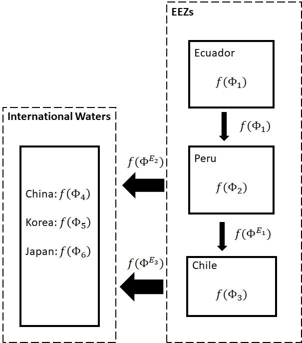
SC9-Obs04
32 Pacific
33 1 Introduction
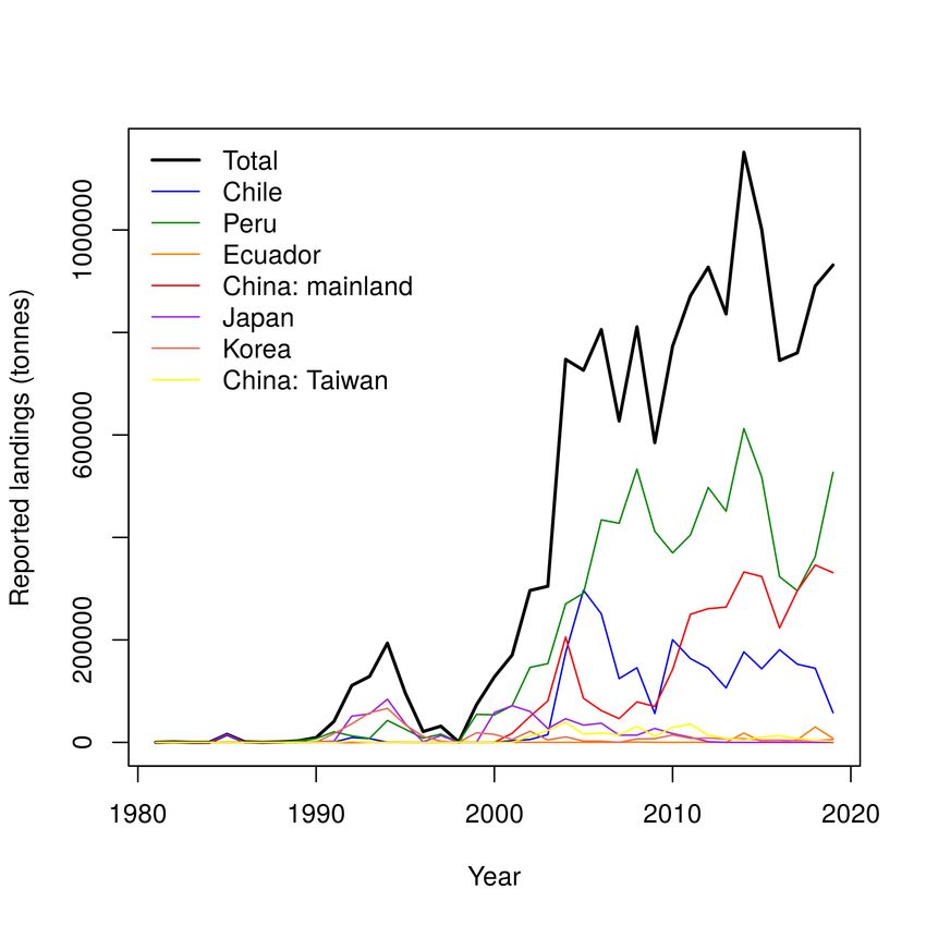
34 The flying jumbo squid fishery extends over the whole Eastern Pacific Ocean yielding
35 the largest volume of landings of any invertebrate fishery worldwide, reaching over a
36 million tonnes in recent years (Robinson et al., 2016). According to FAO records (FAO,
37 2021), in the South Eastern Pacific Ocean (SEP) the fishery started to develop and
38 grow in the early 90s, with the activities of Japanese and Korean fleets in international
39 waters off the jurisdiction of Ecuador, Peru and Chile, and Peruvian fleets in Peru’s
40 Exclusive Economic Zone (EEZ) (Fig. 1). Starting in the 2000s, Chilean and Chinese
41 fleets joined the exploitation in Chilean EEZ and international waters, respectively, and
42 in 2014 Ecuadorian fleets became active in the fishery with landings in the low thousands
43 (Fig. 1).
Figure 1: Historical landing records of the flying jumbo squid in FAO database (FAO,
2021) in the South-Eastern Pacific Ocean.
2
SC9-Obs04

44   A special issue of Fisheries Research (Rodhouse et al., 2016) compiled important biological
45   research including feeding (Rosas-Luis and Chompoy-Salazar, 2016), predators (Rosas-
46   Luis et al., 2016), reproduction (Hernández-Muñoz et al., 2016), and the connection
47   between volume of catches and environmental conditions (Paulino et al., 2016; Robinson
48   et al., 2016). In recent years, discussions regarding method to assess jumbo squid and
49   efforts toward sharing and standardising databases have been made among countries
50   fishing jumbo squid in the SEP (SPRFMO, 2019, 2020). In spite of these efforts, there
51   is still need of an integrated system of observation, modelling and management to secure
52   the continued viability of the fishery (Rodhouse et al., 2016). Currently, there is much
53   interest in generating scientific knowledge leading to an assessment of the abundance and
54   productive capacity of the stock in the SEP region as a whole. This knowledge would be
55   useful to take coordinated and agreed upon management actions aimed at the sustainable
56   exploitation of the stock by the various fleets and countries involved.
57   Life history and population dynamic of cephalopods differ for many harvested fish popula-
58   tions which imposes challenges for assessing and manage their populations. Cephalopods
59   are commonly characterised by very fast growth rates, short life span, high fecundity,
60   continuous spawning during a given season and they show highly phenotypic plasticity
61   as a result of changes in environmental conditions (Arkhipkin et al., 2021). In addition
62   most of cephalopods are semelparous (Hoving et al., 2015), an individual undergoes only a
63   single reproductive cycle after which it dies. Some cepalopods like jumbo squid exhibited
64   high migratory behaviour (Nesis, 1983; Ibáñez and Cubillos , 2007) and age is difficult to
65   asses given the formation of daily increments in hard structures such statolihts. For an
66   assessment viewpoint, in semelparous and fast-growing animals, the estimation of natural
67   mortality became extremely challenging. On the other hand, the time consuming-nature
68   of reading daily increments in cephalopods hard structures make age-based models im-
69   practical to be used in the context of stock assessments. These characteristics preclude
70   the application of routine age and cohort-based stock assessment methods usually applied
71   in teleost fishes. In this context, Arkhipkin et al. (2021) conducted a recent review of
72   cephalopods stock assessment and management and recommended the use of depletion
73   models running at rapid time steps. Such family of stock assessment models can handle
74   rapid life history with short life span in which age and natural mortality are not requires
75   to be estimated beforehand. Depletion models are also less data demanding because they
76   do not require intensive biological sampling or fishery independent data. Roa-Ureta et al.
77   (2021) propose a depletion model for non-closed populations which are particularly use-
78   ful in the context of flying jumbo squid given trans zonal and long migratory behaviour
79   describe for this species.
80   The purpose of this conceptual paper, presented to the 2021 SC SPRFMO Metting, is
81   to propose the construction of a simple and viable regional database to serve as input
82   information for a stock assessment model that would evaluate movements (flows) among

                                                  3
SC9-Obs04
83 sub-regions in the wider SEP region, annual recruitment pulses to each sub-region, average
84 natural mortality rate over the whole region, fishing mortality rates exerted by the various
85 fleets in each sub-region, and total abundance of the stock in the region. The model to be
86 proposed is a new type of generalised depletion model (Roa-Ureta, 2012, 2015; Roa-Ureta
87 et al., 2015, 2019, 2020, 2021) especially modified and adapted to the evaluation of flows
88 among sub-regions. Results of the model will be further exploited to fit a population
89 dynamics model of the general surplus production kind (Roa-Ureta et al., 2019) and a
90 spawners-recruitment model (Roa-Ureta et al., 2021), this latter application depending
91 on the availability of additional biological knowledge or data concerning the maturity
92 ogive.
93 2 Regional Database
94 To apply the depletion model described in the next section, the database that needs to
95 be compiled and curated by Ecuadorian, Peruvian, Chilean, Chinese and Korean fleets,
96 and the Japanese fleet that operated until 2012, consists of complete monthly landings
97 (assumed very close to catches) and fishing effort, plus samples of mean weight in the
98 landings. For purposes of exposition, we are going to assume that the data cover the
99 period of January 2001 to December 2020, because a long time series is more informative,
100 although it should be stressed at this point that the application of the model does not
101 depend on the length of the time series. Note that a general and common template for
102 collecting data in the context of depletion models have been already discussed in the
103 SPRFMO (SPRFMO, 2020).
104 We are also going to assume a single fleet per country though the mode may accom-
105 modate any number of fleets with the subsequent increase in the numerical burden for
106 maximization of the likelihood function. A graphical representation is shown in Fig. 2.
107 In this figure, olive cells ideally are complete, meaning that there could be no gaps (i.e.
108 months with fishing but without recorded data) and the full amount of catch and effort
109 by the fleet has been recorded. On the other hand, yellow cells could have gaps and be
110 based on samples, meaning that the mean weight of squids in the catch was computed
111 by averaging over random samples. In the case of the Japanese fleet all the cells after
112 December 2012 (or an earlier month in that year) will be filled with zeros.
113 One important consideration is that each fleet may report the fishing effort in different
114 units. For instance one fleet may report fishing effort in coarse units such as number of
115 boats or number of fishing trips per month, while another fleet may report fishing effort
116 in more granular units such number of fishing hauls or even hours of fishing per month.
117 As will be shown below, each fleet has its own parameters related to its operations so it
118 is not necessary that all fleets report their fishing effort in the same units. Nevertheless,
119 for every fleet the unit of fishing effort must the same along the entire time series.
4SC9-Obs04
Figure 2: Pictorial representation of the regional database to be compiled and curated to
apply the depletion model.
120 Another important aspect of fitting this type of models is that, although ideally all the
121 catch and all the fishing effort per time step are reported, the existence of a few gaps in
122 the time series of a given fleet may be overcome by using statistical imputation techniques
123 but for this to be acceptable, without seriously compromising the reliability of results,
124 these gaps need to be few and spread over the whole time series.
125 3 Generalised Depletion Model with Flows Among
126 Sub-regions
127 3.1 General model
128 Generalised depletion models are depletion models for open populations with nonlinear
129 dynamics. Regarding the open population aspect, traditional depletion models do not
130 admit inputs of abundance during the fishing and that is the reason they could not
131 be used for multi-annual assessments, since in that case one obvious factor, the annual
132 pulse of recruitment, could not be included in the assessment. Therefore, depletion
133 models were often connected to assessing stocks with intra-annual data, for one season of
134 fishing separately. Generalised depletion models allow any number of exogenous inputs of
135 abundance during the fishing, so they are apt for multi-annual assessments with monthly
136 data (Roa-Ureta, 2015). Regarding the nonlinear dynamics aspect, traditional depletion
137 models assumed a linear relationship between catch as the result, and fishing effort and
138 stock abundance as the causes of the catch. Therefore, it is common with these traditional
139 depletion models to use the catch per unit of effort on the l.h.s of the equation and the
140 abundance dynamics in the r.h.s. of the equation. Generalised depletion models allow
141 for nonlinear dynamics for the effect of fishing effort and stock abundance on catch, and
5SC9-Obs04
142 therefore fishing effort is not used as a standardising quantity but as a predictor on the
143 r.h.s. of the equation. Perhaps more importantly, generalised depletion models allow for
144 a nonlinear effect of stock abundance on the resulting catch, which allows considering
145 phenomena such as hyper-stability (Roa-Ureta, 2012).
146 With those introductory remarks, and assuming a database of 20 years (2001 to 2020)
147 and six fleets, we can now define precisely the model that we propose to assess the jumbo
148 squid stock in the SEP. So let C be the expected total (across all fleets) catch under the
149 model and let t be a month in the time series. Let Et,f be the total fishing effort of fleet
150 f in month t. Then the model states that
f =6
X
Ct = Cf,t
f =1
α1 β1 α2 β2 α3 β2 α4 β4 α5 β5 α6 β6
= k1 E1,t Nt + k2 E2,t Nt + k3 E3,t Nt + k4 E4,t Nt + k5 E5,t Nt + k6 E6,t Nt
"i=t−1 # j=20 !β1
X X
α1 M/2
Ct = k1 E1,t e N0 e−M t − eM/2 C1,i e−M (t−i−1) + I1,j R1,j e−M (t−τ1,j ) ± f (Φ1 ) +
i=1 j=1
"i=t−1 # j=20
!β2
X X
α2 M/2
k2 E2,t e N0 e−M t − eM/2 C2,i e−M (t−i−1) + I2,j R2,j e−M (t−τ2,j ) ± f (Φ2 ) +
i=1 j=1
"i=t−1 # j=20
!β3
X X
α3 M/2
k3 E3,t e N0 e−M t − eM/2 C3,i e−M (t−i−1) + I3,j R3,j e−M (t−τ3,j ) ± f (Φ3 ) +
i=1 j=1
"i=t−1 # j=20
!β4
X X
α4 M/2 −M t M/2 −M (t−i−1) −M (t−τ4,j )
k4 E4,t e N0 e −e C4,i e + I4,j R4,j e ± f (Φ4 ) +
i=1 j=1
"i=t−1 # j=20
!β5
X X
α5 M/2
k5 E5,t e N0 e−M t − eM/2 C5,i e−M (t−i−1) + I5,j R5,j e−M (t−τ5,j ) ± f (Φ5 ) +
i=1 j=1
"i=t−1 # j=20
!β6
X X
α6 M/2
k6 E6,t e N0 e−M t − eM/2 C6,i e−M (t−i−1) + I6,j R6,j e−M (t−τ6,j ) ± f (Φ6 )
i=1 j=1
(1)
151 The monthly catch of each fleet is determined by a proportionality constant, the scaling
152 (k ), which is comparable to catchability (although more general, see Roa-Ureta (2012))
153 having units of effort−1 × abundance−1 , times the fishing effort E modulated by the
154 effort-response parameter α, times stock abundance N modulated by the abundance-
155 response parameter β. Thus, the monthly catch of each fleet is the result of two causes,
156 effort and abundance, with effort being an observed cause and abundance being a latent
157 cause. In the third line of Eq. 1, latent abundance available to each fleet is made explicit
158 and expanded with Pope’s equation (second sum inside parentheses) and the input of
6SC9-Obs04
159 abundance (third sum inside parentheses) corresponding to the annual recruitment (R)
160 to the fleet as a part of the total recruitment (R = R1 + R2 + R3 + R4 + R5 + R6 ) in year
161 j (j = 1, ..., 20, 2001 to 2020) minus or plus a function of immigration and emigration
162 pulse among sub-regions, to be explained below. Parameters N0 and M are the initial
163 abundance (January 2001) and the average (across the whole period) monthly natural
164 mortality rate, respectively, and these two parameters are common to all fleets because
165 they are characteristics of the stock, independent of fishing operations. The variable Ij
166 is an indicator that takes the value of 0 before the input of recruitment and 1 afterwards.
167 Finally, parameters τj are the months in which recruitment happens in year j, which can
168 be different for each fleet.
169 The model has a total of 120 recruitment parameters (20 years × 6 fleets), plus N0 and
170 M, plus six k, α and β parameters, giving a total of 140 free differentiable parameters,
171 before counting immigration and emigration pulses. To tackle this multidimensional
172 optimization problem there would be 1440 pairs of observations of catch and effort (20
173 years × 12 months × 6 fleets). This total data count does not count the months when
174 the fishing is not happening in some fleets because of seasonality of operations.
175 The model in Eq. 1 is the process model, the postulated mechanism linking the true
176 catch Ct to effort and abundance, which is assumed to be fairly complete and exact, with
177 negligible process error. The true catch time series however, are not observed. Instead,
178 random time series χf,t are observed and its expected value is Cf,t . Thus the catch time
179 series are random variables and the stock assessment model is completed with a statisti-
180 cal model where χf,t has a probability density, a specific parametric distribution. In this
181 proposal, two distributions will be implemented for each fleet, normal and lognormal,
182 corresponding with additive or multiplicative hypotheses for the observations of catch.
183 Each fleet’s catch data may have any of the two distribution, giving rise to 26 = 64 com-
184 binations for distributional hypothesis of the total catch distribution. In implementing
185 the normal and lognormal distributions for the fleet’s catch data, adjusted profile approx-
186 imations will be coded to eliminate the dispersion parameters, leading to the following
187 approximate likelihood functions for the data,
T −2 log PT (χt − Ct )2 N ormal
2 i=1
lp (θθ ; {χt , Et }) = P (2)
T −2 log T 2
2 i=1 (log(χt ) − log(Ct )) Lognormal
188 where lp is the negative log-likelihood function, θ is the vector of 140+ parameters,
189 {χt , Et } are the catch and effort data, Ct is the predicted catch according to the model
190 in Eq. 1, and T is the total number of months (T = 240 with 20 years of data). These
191 negative log-likelihood functions are minimised numerically as a function of θ to estimate
192 maximum likelihood parameter values and their covariance matrix. The 140 + ×140+
193 covariance matrix contains the asymptotic standard errors of parameter estimates along
7SC9-Obs04
194 its main diagonal and the covariances/correlations in the off diagonal triangles.
195 In addition to the 140+ differentiable parameters, the model has 20 years × 6 fleets
196 = 140 τ parameters corresponding to the month of recruitment to each fleet in each
197 year, and these τ parameters are non-differentiable. They can be estimated by maximum
198 likelihood by fitting models with alternative τ for each fleet and year combination and
199 selecting the fit that maximises the likelihood. In this proposal the τ parameters will
200 be initially evaluated using the non-parametric catch spike statistics (Roa-Ureta, 2015).
201 After examination of optimization results with this initial timing hypothesis, further
202 hypotheses will be evaluated by changing some of the months of recruitment for some
203 of the fleets. The final best model will be selected as the one with the lowest Akaike
204 Information Criterion (AIC) as well as better numerical, biological realism and statistical
205 quality criteria.
206 3.2 Flows among sub-regions
207 There are several authors that have hypothesised that groups of jumbo squid that differs
208 in life history traits such as maturity and size should represent genetically discrete units,
209 and thus should be treated as isolated stocks for managing purposes (see revision in Ibáñez
210 et al. (2015)). However, many molecular studies have demonstrated that specimens of
211 different sizes in different areas of the South Pacific are genetically identical (Sandoval-
212 Castellanos et al., 2009; Wang et al., 2021). Variations found in life history traits seem
213 to be caused by the large phenotypic flexibility of this species (Hoving et al., 2013).
214 The lack of genetic differences and the migratory behaviour of jumbo squids support the
215 hypothesis that this species composes only one large interconnected stock in the South
216 east Pacific.
217 There are few hypotheses regarding flows and interconnections among sub-regions along
218 the exclusive economic zones (EEZs) and open international seas in the South East Pacific.
219 However, one of the most accepted hypotheses indicates flows in the north-south axis
220 along the cost of Ecuador, Peru and Chile and also a reproductive migration of individuals
221 off shore from Chile and Peru (Ibáñez et al., 2015). We Followed this hypothesis as first
222 approach to modelling the jumbo squid stock in the South east Pacific. An idealised
223 representation of hypothesis is shown in Figure 3.
8SC9-Obs04
Figure 3: Idealised representation of stock flows across sub-regions in an arbitrary υ
month. f (Φ) represents the immigration/emigration flows on each sub-region/fleets
224 The f (Φf ) terms in Eq. 1 account for the possibility that part of the stock moves from
225 one sub-region to another sub-region at specific months during the period covered by time
226 series of data. To simplify the exposition, consider the idealised situation represented in
227 Fig. 3. On an arbitrary month υ, there are minor pulses from Ecuador to Peruvian EEZs
228 and also from Peru to Chilean EEZ. In the same month (υ), larger pulses happen from
229 the Peruvian EEZs and from Chilean EEZs to international waters offshore. The catch
230 and effort data, when of sufficient quality, may contain information on immigration and
231 emigration that allow estimation of the magnitude of those pulses as demonstrated in
232 Roa-Ureta et al. (2021).
233 Let enumerate the fleets in eq. 1, as Ecuador (1), Peru (2), Chile (3), China (4), Korea
234 (5) and Japan (6), then, the modelled flows on each sub-region/fleets are as follows:
9SC9-Obs04
235 Ecuador:
" j=20 #
X
−M (t−υ)
f (Φ1 ) = −Υ Φ1,j e (3)
j=1
236 where Υ is an indicator variable that takes the value of 1 in the month υ where flows
237 among fleets occurs, and takes a value of 0 otherwise. Note the simplified assumption
238 that all flows among sub-regions occur at the same month (υ).
239 The Peruvian sub-region included the most complex case in which an immigration input
240 is received from Ecuador, but this sub-region also generates emigrations for Chile EEZ
241 (which magnitude is refers as ΦE E2
j ) and to international waters (Φj ) as follows,
1
242 Peru:
" j=20 j=20 j=20
#
X X X
f (Φ2 ) = Υ Φ1,j e−M (t−υ) − ΦE1 −M (t−υ)
j e − ΦE2 −M (t−υ)
j e
j=1 j=1 j=1
" j=20 #
X
E2 −M (t−υ)
=Υ (Φ1,j − ΦE
j − Φj )e
1
j=1 (4)
" j=20 #
X
=Υ (Φ2,j )e−M (t−υ)
j=1
243 where (Φ2,j = Φ1,j − ΦE E2
j − Φj ) represents the net flux from the EEZ Peruvian sub-
1
244 region in the year j. Note the sign of parameter Φf,j is indicating the importance of
245 either immigration or emigration on each particular sub-region and year.
246 Note that Peruvian vessels had fished for Jumbo squid in international waters (SC7-
247 Doc33, 2019). However, on this first modelling approach, we considered these catches
248 negligible in comparison with Peru’s catches on its EEZ. Nevertheless, the proposed
249 modelling framework can be easily adapted to include any other fleet in international
250 waters if adequate data are available.
251 Likewise, in the case of the Chilean sub-region, we consider an immigration from Peru
252 (ΦE E3
j ) and an emigration to international waters defined as (Φj ). Then, the flow model
1
253 for Chile can be described as,
254 Chile:
10SC9-Obs04
" j=20 j=20
#
X X
1 −M (t−υ) 3 −M (t−υ)
f (Φ3 ) = Υ ΦE
j e − ΦE
j e
j=1 j=1
" j=20 #
X
E3 −M (t−υ)
=Υ (ΦE
j − Φj )e
1
j=1 (5)
" j=20 #
X
=Υ (Φ3,j )e−M (t−υ)
j=1
255 In the case of the International sub-region, we consider an immigration from Peru (ΦjE2 )
256 and another from Chile (ΦE j ). However, these immigration pulses are shared among the
3
257 three international fleets. In general terms, the Peruvian immigration to international
258 waters can be divided among the Chinese (4), Korean (5) and Japanese (6) fleets as
259 follows: ΦjE2 = ΦE E2 E2
4,j j + Φ5,j j + Φ6,j j . Likewise, the Chilean immigration to international
2
260 waters can be divided among fleets as, ΦE 3 E3 E3 E3
j = Φ4,j j + Φ5,j j + Φ6,j j . Note from data alone,
261 it is impossible to know which amount of immigration is fished by which international
262 fleet (e.g ΦE E3
f,j j , Φf,j j ). However, it is possible to know from data the net flux from each
2
263 international fleet in the same manner as we did in the other sub-regions above:
264 China:
" j=20 j=20
#
X X
2 −M (t−υ) 3 −M (t−υ)
f (Φ4 ) = Υ ΦE
4,j e − ΦE
4,j e
j=1 j=1
" j=20 #
X (6)
=Υ Φ4,j e−M (t−υ)
j=1
265 Korea:
" j=20 j=20
#
X X
E2 −M (t−υ) E3 −M (t−υ)
f (Φ5 ) = Υ Φ5,j e − Φ5,j e
j=1 j=1
" j=20 #
X (7)
=Υ Φ5,j e−M (t−υ)
j=1
266 and Japan:
11SC9-Obs04
" j=12 j=12
#
X X
2 −M (t−υ) 3 −M (t−υ)
f (Φ6 ) = Υ ΦE
6,j e − ΦE
6,j e
j=1 j=1
" j=12 #
X (8)
=Υ Φ6,j e−M (t−υ)
j=1
267 where Φ4,j , Φ5,j and Φ6,j , are the net immigration fluxes on the year j by China, Korea
268 and Japan, respectively.
269 In practice, only the larger emigration/immigration pulses would be estimated reliably
270 enough from the model and the data. With further reference to eq. (1), on an arbitrary
271 month all sub-regions receive an input of abundance corresponding to annual recruit-
272 ment, i.e. squids that grow to become vulnerable to the fishing gear, and there are no
273 emigration/immigration pulses, thus in a month like this Eq. 1 would have the Φf terms
274 evaluating to zero by virtue of indicator variable Υ.
275 4 General Surplus Production Model for the
276 Region
277 The depletion model above allows direct estimation of 140 parameters but it also permits
278 posterior calculation of derived parameters and predictions such as monthly fishing mor-
279 tality by fleet (from Baranov catch equation), regional abundance and regional biomass
280 per month in absolute terms. The latter two predictions are estimated with standard
281 errors using the Delta method. By selecting one of the monthly regional biomass esti-
282 mates per year (preferably the biomass in the month that on average across the years,
283 produces the estimate with the lowest standard error) and by appending the regional
284 total catch for the years before the time series covered with the depletion model, it is
285 possible to estimate a general surplus production model of the Pella-Tomlinson type. In
286 our approach this is done with a non-Bayesian hierarchical inference method based on
287 hybrid likelihood functions (Roa-Ureta et al., 2015). The Pella-Tomlinson model is
p−1 !
By−1
By = By−1 + rBy−1 1− − Cy−1 , p > 1, y1 ≤ y ≤ yend (9)
K
288 where r is the intrinsic population growth rate, p is the symmetry of the production
289 function, K is the carrying capacity, By is the biomass estimated in the depletion model,
290 and Cy−1 is the total annual catch during the previous fishing season.
291 The annual biomass and its standard deviation from fitting the depletion model and
12SC9-Obs04
292 the annual biomass predicted by the Pella-Tomlinson model are linked through a hybrid
293 (marginal-estimated) likelihood function,
y
!
end
1X (B̂y − By )2
`HL (θθ P T |{B̂y }) ∝ − log(2πSB̂2 y ) + (10)
2 y SB̂2
1 y
294 where θ = {By0 , K, r, p} is the vector of parameters of the Pella-Tomlinson model in Eq.
295 9 plus one additional parameter for biomass in the year prior to the first year in the
296 time series, 2000, SB̂2 are the distinct numerical estimates of standard deviations of each
y
297 annual biomass estimate from the fitted depletion model (replacing the unknown distinct
298 true standard deviations), B̂y are the likelihood estimates of annual biomass from the
299 fitted depletion model, and By are the true annual biomass according to Eq. 9.
300 With reference to θ , models could be fit where By0 is a distinct parameter or where it
301 is set to be equal to K. In the second option it is assumed that the stock was at the
302 carrying capacity when the annual time series (that goes much more back in time than
303 the depletion model time series) started. Thus the first option is a fit a 4-parameters
304 model while the second option is a fit of 3-parameters model. The second option is useful
305 because convergence of the fit may not need to be burdened with four parameters to
306 estimate and also because the true biomass at the start of the annual time series, By0 ,
307 is the least important parameter for management of the stock at the current time. To
308 determine which of the two options is better for the biomass observations it is possible
309 to use the model with the lowest AIC.
310 From the fit of Pella-Tomlinson model, we compute several biological reference points
311 depending on the prevailing dynamics of the stock. Those reference points were the
312 MSY,
M SY = rK(p − 1)p−p/(p−1) (11)
313 the biomass at the MSY,
BM SY = Kp1/(1−p) (12)
314 and the latent productivity,
p−1 !
pp/(p−1
By By
Ṗ = γM SY 1− ,γ = (13)
K K p−1
315 For all those biological reference points, standard errors are computed using the delta
316 method.
317 With reference to the latent productivity (Quinn and Deriso, 1990), this is a biological
318 reference point analogous to the MSY, but while the MSY is a constant, the latent
319 productivity varies with the biomass of the stock. Thus the latent productivity is more
13SC9-Obs04
320 relevant for stocks that tend to fluctuate because of environmental forces or because of
321 their intrinsic population dynamics. For instance, in Roa-Ureta et al. (2015) we found that
322 the stock under study was fluctuating because of a high value of the intrinsic population
323 growth rate, r. In another case (Roa-Ureta et al., 2021) we found that the stock was
324 undergoing cyclic fluctuations due to an unstable equilibrium point in the spawners-
325 recruitment relationship. Thus the MSY was not applicable in those cases and it was
326 actually an excessive harvest rate.
327 5 Final Remarks
328 • Data regarding monthly catches and average individually weight on each sub-region
329 and fishing fleet will be needed on a first modelling approach. Future and more
330 intensive biological sampling (e.g maturity) will allow coupling a depletion model
331 with productivity derive from a stock-recruitment relationship.
332 • Model specification for flows can be adjusted to different competing hypotheses
333 regarding immigration/emigration among sub-regions. These hypotheses can be
334 evaluated in the context of model selection.
335 • The proposed modelling framework is flexible enough to capture the main features
336 of the jumbo squid such as fast growth rate, inter-connectivity within the stock
337 among several sub-regions and fleets with different units for effort.
338 • Collaboration among different countries in the SPRFMO will be crucial for the
339 implementation of the proposed modelling framework. Main aspects of such collab-
340 oration should be based on data curation and data sharing in common templates,
341 agreements regarding extension of the data used and the selection on the main
342 migratory (flows) hypotheses to be tested.
343 6 Acknowledgements
344 We thank C.M. Ibáñez for his helpful discussion regarding the hypotheses of jumbo squids
345 migrations among sub-regions and to Renato Gozzer for his comments and suggestions
346 that improved an early version of this report.
347 References
348 Arkhipkin, A.I., Hendrickson, L.C., Payá, I., Pierce, G.J., Roa-Ureta, R.H., Robin, J-P.,
349 Winter, A. 2021. Stock assessment and management of cephalopods: advances and
14SC9-Obs04
350 challenges for short-lived fishery resources. ICES Journal of Marine Science 78, 714–
351 730.
352 Berger, T., Sibeni, F., Calderini, F. 2021. FishStatJ, a tool for fishery statistics analysis,
353 release 4.01.5. FAO, Fisheries Division, Rome.
354 Congcong Wang, Gang Li, Hao Xu
355 Hernández-Muñoz, A.T., Rodrı́guez-Jaramillo, C., Mejı́a-Rebollo, A., Salinas-Zavala,
356 C.A. 2016. Reproductive strategy in jumbo squid Dosidicus gigas (D’Orbigny, 1835):
357 A new perspective. Fisheries Research 173, 159–168.
358 Hoving, H.J.T., Gilly, W.F., Markaida, U., Benoit-Bird, K.J., -Brown, Z.W., Daniel, P.,
359 Field, J.C., Parassenti, L., Liu, B., Campos, B. 2013. Extreme plasticity in life-history
360 strategy allows a migratory predator (jumbo squid) to cope with a changing climate.
361 Global change biology 19, 2089–2103.
362 Hoving, H.J.T., Laptikhovsky, V.V., Robison, B.H. 2015. Vampire squid reproductive
363 strategy is unique among coleoid cephalopods. Current Biology, 25(8), R322–R323.
364 Ibáñez, C.M., Cubillos, L.A. 2007. Seasonal variation in the length structure and repro-
365 ductive condition of the jumbo squid Dosidicus gigas (d’Orbigny, 1835) off central-south
366 Chile. Scientia Marina, 71(1), 123–128.
367 Ibáñez, C.M., Sepúlveda, R.D., Ulloa, P., Keyl, F., Pardo Gandarillas, M.C., 2015. The
368 biology and ecology of the jumbo squid Dosidicus gigas (Cephalopoda) in Chilean
369 waters: a review. Latin American Journal of Aquatic Research, 43, 402–414.
370 Nesis, K.N. 1983. Dosidicus gigas In: P.R. Boyle (ed.). Cephalopod life cycles, Vol. 1.
371 Species accounts. Academic Press, London, pp. 216–231.
372 Robinson, C.J., Gómez-Gutiérrez, J., Markaida, U., Gilly, W.F. 2016. Prolonged decline
373 of jumbo squid (Dosidicus gigas) landings in the Gulf of California is associated with
374 chronically low wind stress and decreased chlorophyll a after El Niño 2009–2010. Fish-
375 eries Research 173, 128–138.
376 Rodhouse, P.J.K., Yamashiro, C., Arguelles, J. 2016. Introduction. Jumbo squid in the
377 eastern Pacific Ocean: A quarter century of challenges and change. Fisheries Research
378 173, 109–102.
379 Rosas-Luis, R., Chompoy-Salazar, L. 2016. Description of food sources used by jumbo
380 squid Dosidicus gigas (D’Orbigny, 1835) in Ecuadorian waters during 2014. Fisheries
381 Research 173, 139–144.
15SC9-Obs04
382 Rosas-Luis, R., Loor-Andrade, P., Carrera-Fernández, M., Pincay-Espinoza, J.E., Vinces-
383 Ortega, C., Chompoy-Salazar, L. 2016. Cephalopod species in the diet of large pelagic
384 fish (sharks and billfishes) in Ecuadorian waters. Fisheries Research 173, 159–168.
385 Paulino, C., Segura, M., Chacón, G. 2016. Spatial variability of jumbo flying squid (Do-
386 sidicus gigas) fishery related to remotely sensed SST and chlorophyll-a concentration
387 (2004-2012). Fisheries Research 173, 122–127.
388 Roa-Ureta, R.H. 2012. Modeling In-Season Pulses of Recruitment and Hyperstability-
389 Hyperdepletion in the Loligo gahi Fishery of the Falkland Islands with Generalized
390 Depletion Models. ICES Journal of Marine Science 69, 1403–1415.
391 Roa-Ureta, R.H., 2015. Stock assessment of the Spanish mackerel (Scomberomorus com-
392 merson) in Saudi waters of the Arabian Gulf with generalized depletion models under
393 data-limited conditions. Fisheries Research 171, 68–77.
394 Roa-Ureta, R.H., Molinet, C., Bahamonde, N., Araya, P. 2015. Hierarchical statistical
395 framework to combine generalized depletion models and biomass dynamic models in
396 the stock assessment of the Chilean sea urchin (Loxechinus albus) fishery. Fisheries
397 Research 171, 59–67.
398 Roa-Ureta, R.H., Santos, M.N., Leitão, F. 2019. Modelling long-term fisheries data to
399 resolve the attraction versus production dilemma of artificial reefs. Ecological Modelling
400 407, 108727.
401 Roa-Ureta, R.H., Henrı́quez, J., Molinet, C. 2020. Achieving sustainable exploitation
402 through co-management in three Chilean small-scale fisheries. Fisheries Research 230,
403 105674.
404 Roa-Ureta, R.H., Fernández-Rueda, M.P., Acuña, J.L., Rivera, A., González-Gil, R.,
405 Garcı́a-Flórez, L. 2021. Estimation of the spawning stock and recruitment relationship
406 of Octopus vulgaris in Asturias (Bay of Biscay) with generalized depletion models:
407 implications for the applicability of MSY. ICES Journal of Marine Science. pdf.
408 Sandoval-Castellanos, E., Uribe-Alcocer, M. and Dı́az-Jaimes, P. 2009. Lack of genetic
409 differentiation among size groups of jumbo squid (Dosidicus gigas). Ciencias marinas,
410 35(4), 419–428.
411 SC7-Doc33. 2019. Peru’sAnnual report(SPRFMO Area). 7th MEETING OF THE SCI-
412 ENTIFIC COMMITTEE, La havana, Cuba.
413 SPRFMO. 2019. SPRFMO SC 2nd Squid Workshop Report. 20 p. Wellington, New
414 Zealand 2019.
16SC9-Obs04
415 SPRFMO. 2020. 8th Scientific Committee meeting report. 76 p. Wellington, New Zealand
416 2020.
417 Quinn, T.J., Deriso, R. 1990. Quantitative Fish Dynamics. Oxford University Press, NY.
418 Wang, C., Li, G., Xu, H. 2021. China genetics study of Jumbo flying squid, methods and
419 results. South Pacific Regional Fisheries Management Organization. Technical Report,
420 10 p.
17You can also read