A decade of glaciological and meteorological observations in the Arctic (Werenskioldbreen, Svalbard) - ESSD
←
→
Page content transcription
If your browser does not render page correctly, please read the page content below
Earth Syst. Sci. Data, 14, 2487–2500, 2022
https://doi.org/10.5194/essd-14-2487-2022
© Author(s) 2022. This work is distributed under
the Creative Commons Attribution 4.0 License.

             A decade of glaciological and meteorological
        observations in the Arctic (Werenskioldbreen, Svalbard)
           Dariusz Ignatiuk1 , Małgorzata Błaszczyk1 , Tomasz Budzik1 , Mariusz Grabiec1 , Jacek A. Jania1 ,
                  Marta Kondracka1 , Michał Laska1 , Łukasz Małarzewski1 , and Łukasz Stachnik2
                    1 Faculty of Natural Sciences, University of Silesia in Katowice, Katowice, 40-007, Poland
       2 Faculty   of Earth Sciences and Environmental Management, University of Wrocław, Wrocław, 50-137, Poland
                    Correspondence: Dariusz Ignatiuk (dariusz.ignatiuk@us.edu.pl) and Marta Kondracka
                                                 (marta.kondracka@us.edu.pl)
                                 Received: 23 December 2021 – Discussion started: 5 January 2022
                             Revised: 22 April 2022 – Accepted: 30 April 2022 – Published: 1 June 2022

       Abstract. The warming of the Arctic climate is well documented, but the mechanisms of Arctic amplification
       are still not fully understood. Thus, monitoring of glaciological and meteorological variables and the environ-
       mental response to accelerated climate warming must be continued and developed in Svalbard. Long-term me-
       teorological observations carried out in situ on glaciers in conjunction with glaciological monitoring are rare
       in the Arctic and significantly expand our knowledge about processes in the polar environment. This study
       presents glaciological and meteorological data collected for 2009–2020 in southern Spitsbergen (Werenskiold-
       breen). The meteorological data are composed of air temperature, relative humidity, wind speed, short-wave
       and long-wave upwelling and downwelling radiation on 10 min, hourly and daily resolution (2009–2020). The
       snow dataset includes 49 data records from 2009 to 2019 with the snow depth, snow bulk density and snow
       water equivalent data. The glaciological data consist of seasonal and annual surface mass balance measure-
       ments (point and glacier-wide) for 2009–2020. The paper also includes modelling of the daily glacier surface
       ablation (2009–2020) based on the presented data. The datasets are expected to serve as local forcing data
       in hydrological and glaciological models as well as validation of calibration of remote sensing products. The
       datasets are available from the Polish Polar Database (https://ppdb.us.edu.pl/, last access: 24 May 2022) and
       Zenodo (https://doi.org/10.5281/zenodo.6528321, Ignatiuk, 2021a; https://doi.org/10.5281/zenodo.5792168, Ig-
       natiuk, 2021b).

1   Introduction                                                    Schuler et al., 2014; Isaksen et al., 2016; Vikhamar-Schuler
                                                                    et al., 2016; Walczowski et al., 2017; Osuch and Wawrzy-
Long-term meteorological observations carried out in situ           niak, 2017; Førland et al., 2020; Wawrzyniak and Osuch,
on glaciers in conjunction with glaciological monitoring are        2020), which causes progressive and ongoing changes in the
rare in the Arctic and may be used to expand knowledge              cryosphere (Błaszczyk et al., 2013; Wawrzyniak et al., 2016;
about processes in the polar environment. Terrestrial mete-         Box et al., 2019; Grabiec et al., 2018; Nuth et al., 2019; van
orological monitoring alone does not always adequately ad-          Pelt et al., 2019; Schuler et al., 2020; Błaszczyk et al., 2021).
dress the needs of numerical modelling as well as valida-           According to the data published in SIOS data access por-
tion and calibration of satellite products regarding glaciers       tal (https://sios-svalbard.org/, last access: 24 May 2022) and
(Pellicciotti et al., 2014; Gabbi et al., 2014). The warming        the meteorological bulletin “Spitsbergen-Hornsund” (https:
of the Arctic climate is well documented, but the mecha-            //hornsund.igf.edu.pl/weather/, last access: 24 May 2022),
nisms of Arctic amplification are still not fully understood        2020 was the year with the warmest summer in the history
(IPCC, 2019). Both, climate and ocean variables have fluc-          of instrumental observations in Svalbard. (The mean June–
tuated in Svalbard in recent decades (Nordli et al., 2014;

Published by Copernicus Publications.
2488 D. Ignatiuk et al.: A decade of glaciological and meteorological observations in the Arctic
July–August temperature was 7.2 ◦ C, about 3 ◦ C above the
climatological normal at the Svalbard Airport meteorolog-
ical station.) In Hornsund the same summer months mean
was 4.8 ◦ C (only 1.2 ◦ C higher than the local normal). The
highest air temperature since the beginning of measurements
was recorded on 25 July 2020: 21.7 and 16.5 ◦ C at Sval-
bard Airport and the Polish Polar Station in Hornsund re-
spectively. Moreover, in 2019 the sea ice area on the Arc-
tic Ocean reached the second minimum extent in the history
of satellite measurements since 1979 (Yadav et al., 2020).
While the summer of 2021 was colder and the minimal Arc-
tic sea ice extent significantly larger, acceleration of the cli-
mate warming trend is proved despite interannual variations
(Hanssen-Bauer et al., 2019). Such acceleration causes sig-
nificant changes in the cryosphere of Svalbard and is partic-
ularly reflected in the faster melting of glaciers and thawing
of the permafrost (Schuler et al., 2020; Christiansen et al.,
2021). It also stimulates faster energy and mass exchange
between the atmosphere, cryosphere and ocean. The above
examples of transition in air temperature, sea ice extent or
glacier and permafrost melting demonstrate regional differ-
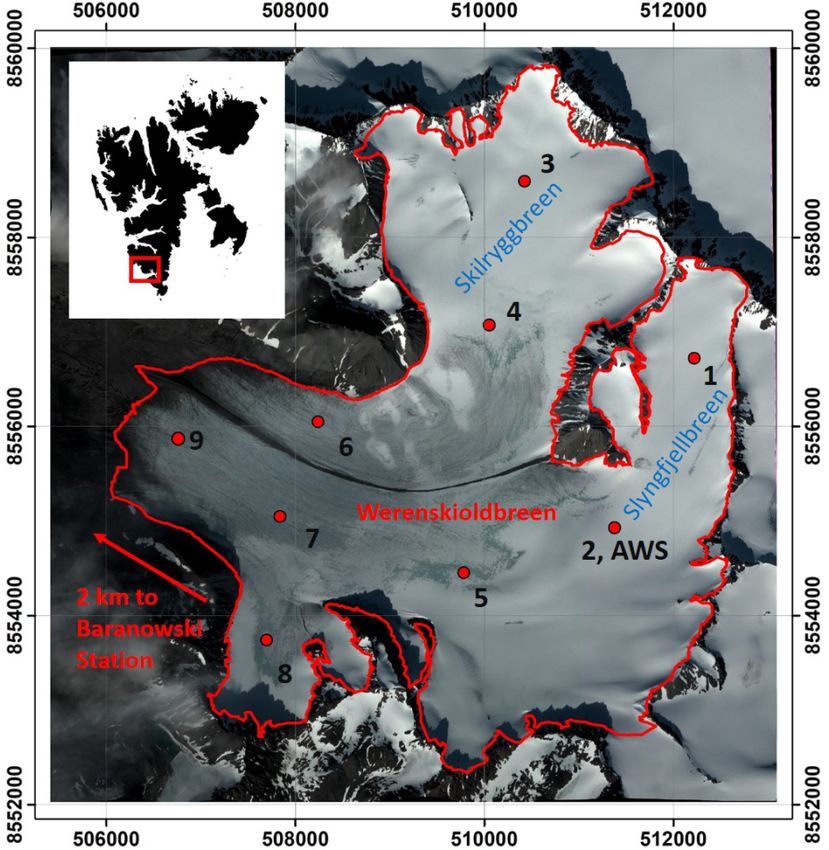
ences in climate warming and subsequently response of other Figure 1. Location of mass-balance stakes (1–9) for 2009–2020
environmental components. Therefore, monitoring of such and the automatic weather station (AWS) on Werenskioldbreen
parameters and the environmental response to climate change (background: GeoEye, 10 August 2010).
is recommended to be carried out in Svalbard, where climate
warming is one of the most dynamic (Nordli et al., 2014;
Isaksen et al., 2016). Long-term observations allow for better moraine. Both facilities greatly simplify the accessibility and
quantification of observed changes and facilitate more pro- logistics of research and monitoring projects.
found understanding of these changes. This study presents
the unique Arctic glaciological and meteorological data col-
3 Instruments and methodology
lected for 2009–2020 in southern Spitsbergen.
3.1 Meteorological monitoring
2 Study area The automatic weather station (AWS) is located at an alti-
tude of 380 m above sea level (Fig. 1), close to the aver-
Werenskioldbreen is a well-studied, polythermal glacier lo- age equilibrium line altitude (ELA) for the years 1959–2008
cated in South Spitsbergen (Fig. 1) (Baranowski, 1982; Pälli (Noël et al., 2020). The station was installed on the glacier on
et al., 2003; Grabiec et al., 2012; Ignatiuk et al., 2015; Stach- 15 April 2010. The AWS was mounted on a long steel mast
nik et al., 2016a, b; Sułowicz et al., 2020). This valley-type placed in the ice drilling hole (ca. 6 m deep). In the follow-
glacier covered an area of 27.1 km2 in 2008 (Ignatiuk et al., ing years, as ablation progressed, the sensors were lowered
2015) and 25.7 km2 in 2017 (current study) in a catchment or the mast was replaced with a new one in close proximity
area of 44 km2 . Werenskioldbreen is divided by a medial to the original location. The recording of variables (air tem-
moraine into the south-eastern part Slyngfjellbreen and the perature, humidity, wind speed, short-wave and long-wave
northern part Skilryggbreen accumulation area (Fig. 1). The radiation) started on 17 April 2010 (Table 1). The Kipp &
glacier’s forefield is closed by a distinct arc of the ice-cored Zonnen CNR4 consists of two CM3 pyranometers, two CG3
terminal moraine with one river gorge. Such a hydrologi- pyrgeometers and temperature sensors (PT100). Pyranome-
cal system allows the glacier basin to be treated as a well- ters (180◦ solid angle) have a glass dome and measure radia-
defined research laboratory for many hydrological and inter- tion in the range from 300 to 2800 nm. One of the pyranome-
disciplinary studies (Majchrowska et al., 2015; Stachnik et ters directed upwards measures downwelling radiation, and
al., 2016b; Łepkowska and Stachnik, 2018; Gwizdała et al., the second one directed downwards measures solar radia-
2018; Stachnik et al., 2019; Osuch et al., 2022). The glacier tion reflected from the earth’s surface (upwelling radiations).
is situated 15 km to the north from the Polish Polar Sta- Pyrgeometers (180–150◦ solid angle) have silicone windows,
tion Hornsund. The Stanisław Baranowski Spitsbergen Polar which allow radiation measurements in the range from 4500
Station (University of Wrocław), a small field station, is lo- to 42 000 nm. Like the pyranometers, the pyrgeometers point
cated at the southern edge of the Werenskioldbreen terminal in opposite directions (upwards and downwards). One of the
Earth Syst. Sci. Data, 14, 2487–2500, 2022 https://doi.org/10.5194/essd-14-2487-2022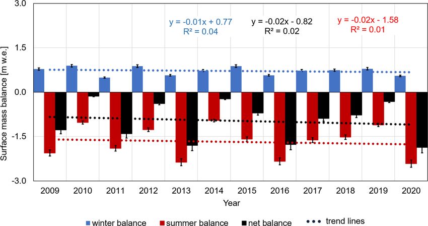
D. Ignatiuk et al.: A decade of glaciological and meteorological observations in the Arctic                                  2489

pyrgeometers measures the long-wave radiation coming from          glacier-wide surface mass balance, snow depth, bulk snow
the atmosphere, the second one the long-wave radiation from        density and SWE at the measuring points.
the ground surface. In 2016, the A100R cup anemometer was             The analyses of the glacier’s surface were based on alti-
replaced with the Gill WindSonic sensor, which allowed for         tude zones determined from digital elevation models (DEM).
measuring wind speed. Damaged sensors were replaced dur-           Two DEMs with geoidal height (EGM2008) were used, one
ing the spring or autumn service to maintain data continuity.      generated from SPOT image acquired on 1 September 2008
   In the years 2010–2011, the sampling time was 1 min. Due        (Ignatiuk et al., 2015) for the years 2008–2019 and Pleiades
to high energy demand during the polar night, the sampling         high-resolution images taken on 20 August 2017 (Błaszczyk
time was changed to an instantaneous measurement every             et al., 2019) for year 2020.
10 min. Calibration and testing of sensors were performed
regularly during spring expeditions based on the infrastruc-
                                                                   4     Meteorological observations
ture of the Polish Polar Station Hornsund.
                                                                   4.1    Air temperature and radiation

3.2   Glaciological monitoring                                     The air temperature data forms the most homogeneous se-
                                                                   ries for 2010–2016 (Fig. 2a). For 2017–2020 the data gaps
In 2009–2010, nine mass-balance stakes were installed on           were already significant due to a series of failures of the in-
the Werenskioldbreen. The locations have been chosen to            struments. Also, for 2010–2016, net radiation balance data
cover the elevation range from 117 to 515 m a.s.l. to create al-   (short- and long-wave radiation) are available (Fig. 2b and
titudinal profiles along the northern and southern tributaries     c). For 2017–2020, radiation data included only downwelling
of the glacier (Fig. 1).                                           short-wave radiation.
   The stakes, 6–8 m long, were embedded in the glacier by a          For years with full data continuity (Fig. 2a), air tempera-
steam drilling rig or by Kovacs ice coring system (ICS). The       ture monthly and yearly averages were calculated and then
mass-balance stakes were measured twice a year (spring–            compared with the data from the Polish Polar Station Horn-
autumn, 2009–2013) during the winter maximum accumu-               sund (Wawrzyniak and Osuch, 2020). The average differ-
lation (April–May) and at the end of the ablation season           ence in the annual temperature (2011, 2012, 2014 and 2015)
(September–October) or once a year (at spring, since 2014).        between the glacier (380 m a.s.l.) and the Polish Polar Sta-
The measure of winter accumulation was determined during           tion Hornsund (8 m a.s.l.) was −2.7 ◦ C, which gives an av-
the spring campaigns. The properties of snow cover (bulk           erage temperature lapse rate of 0.72 per 100 m (annual val-
snow density, snow depth and snow water equivalent (SWE))          ues vary from 0.55 to 0.80 per 100 m). We have calculated
were measured in snow pits (a 100 cm3 snow gauge by Win-           the significance of the trend presented in this study using
ter Engineering was used to determine the snow density of          the non-parametric modified Mann–Kendall test (Hamed and
subsequent layers) or shallow core boreholes (ICS). Dur-           Rao, 1998) while considering the effect of autocorrelation of
ing the measurements, repeated soundings of the snow depth         time series. The slope of the trend was calculated using Sen’s
were also performed with avalanche probes. In the absence of       method (Sen, 1968). The test indicated the statistically signif-
the autumn campaign, boreholes have been drilled near each         icant increasing temperature trend in the period 2010–2016
stake in order to accurately determine the amount of summer        (with the significance level α = 0.05 and p value = 0.036),
ablation and possible summer accumulation. Measurements            and taking into account the 12-month seasonality the Sen’s
during the autumn campaign did not always take place after         slope was 0.02. Gaps in the data were filled based on the rela-
or at the end of the ablation season. This was due to the logis-   tions between air temperature measured on the PPS in Horn-
tics of the expeditions and the extension of the ablation sea-     sund and air temperature on the WRN glacier (R 2 = 0.96).
son. In the case of availability of data from the SR50A sen-       According to the Wawrzyniak and Osuch (2020), the esti-
sor, ablation or accumulation corrections were also made if        mated slope of trend for air temperature between 1979 and
the winter or summer season ended later than the date of field     2018 at the Hornsund station was estimated as 1.14 ◦ C per
observations. Some of the ablation stakes have been damaged        decade. Increasing distance between the glacier surface and
every few years. They have been broken by wind, polar bears,       the sensors during the season is affecting the air temperature
melt out from the ice or been buried by snow. The network          measurements. Periodic measurements of the vertical tem-
of ablation stakes was supplemented and renovated during           perature gradient between 0.5 and 4 m carried out at the AWS
maintenance visits. Unfortunately, recent years have resulted      indicate that the air temperature in the atmospheric boundary
in large gaps in measurements due to the pandemic travel           layer changes by about 0.2 ◦ C m−1 during the ablation sea-
restrictions (years 2020 and 2021). Detailed information on        son. Downwelling short-wave radiation reaches its maximum
the temporal availability of glaciological data is presented in    during the middle of the polar day (June). Its annual course
Table 2.                                                           is governed by the occurrence of polar day and night, while
   Based on the data collected, the following glaciologi-          its daily course is governed the height of the sun above the
cal variables are available: seasonal and annual point and         horizon. The reflected short-wave radiation (upwelling) is a

https://doi.org/10.5194/essd-14-2487-2022                                         Earth Syst. Sci. Data, 14, 2487–2500, 2022
2490 D. Ignatiuk et al.: A decade of glaciological and meteorological observations in the Arctic
Table 1. Automatic weather station (AWS) sensors specification (Werenskioldbreen, Svalbard). All sensors were set in the spring so that
they were about 1.5 m above the snow surface, and height has been varied during the season.
Variable Sensor/producer Operating range Accuracy Period of operation (per-
cent of gaps in dataset)
Air temperature 107/Campbell Scien- −35. . . +50 ◦ C ±0.2 ◦ C (over range Apr 2010–May 2016 (6 %)
tific 0. . . 50 ◦ C)
Air temperature HMP155 −80. . . +60 ◦ C ± Accuracy at −80. . . May 2016–Dec 2019
(PT100)/Vaisala +20 ◦ C (0.226–0.0028 (60 %)
× temperature) ◦ C
Relative humidity HOBO/ONSET COM- 0 %. . . 100 % RH ±2.5 % (10 %–90 % Mar 2011–Sep 2011 (0 %)
PUTER RH);
±5 % (below 10 % and
above 90 %)
Relative humidity HMP45AC/Vaisala 0 %. . . 100 % ±2 % (0 %–90 % RH) May 2016–Aug 2019
±3 % (90 %–100 % (55 %)
RH)
Wind speed A100R/Vector Instru- 0. . . 75 m s−1 ±0.1 m s−1 (0.3– Sep 2010–May 2016
ments 10 m s−1 ); (14 %)
±1 % (10–55 m s−1 );
±2 % (> 55 m s−1 )
Radiation CNR4 /Kipp&Zonen Short wave: Pyranometer: uncer- Sep 2010–May 2016 (1 %)
– short wave: down- 300–2800 nm tainty in daily total
welling and up- Long wave: < 5%
welling 4500–42 000 nm Pyrgeometer: uncer-
tainty in daily total
– long wave: down- < 10 %
welling and up- ±6 % (−40–80 ◦ C)
welling ±25 W m−2 at
1000 W m−2
Data logger CR1000/Campbell Sci- −40 to 50 ◦ C Apr 2010– May 2020 (–)
entific
Ablation and accumu- SR50/Campbell Scien- 0.5–10 m ±1 cm or 0.4 % Sep 2010–Dec 2019 (–)
lation tific
function of the surface albedo. In the spring and early sum- water under the station or the presence of sediment or cry-
mer, we observed the highest values of reflected radiation oconite. Both of these situations were observed at the AWS.
due to the presence of snow cover on the glacier. In the fur- In the view of the CNR4 sensor (180◦ ), there is also a mast
ther part of the ablation season (July–August), we noticed a with a logger, sensors and a solar panel, which cause dis-
sudden decrease in reflected radiation (Fig. 2b) as a result of tortions in the observations. These problems are difficult to
the disappearance of snow cover at the measurement site (i.e. eliminate. Assuming the homogeneity of the surface around
the AWS) and the appearance of glacial ice on the surface. the AWS, increasing the distance of the CNR4 sensor from
The decrease in upwelling short-wave radiation can be slight the glacier surface should not affects its measurements.
(e.g. 2012) when the melting of snow cover occurs mainly as
a result of surface ablation or abrupt (e.g. 2015) when sig-
nificant rainfall led to a sudden change in the albedo on the 4.2 Other variables
glacier. The maximum values of downwelling or upwelling The AWS measured relative humidity, wind speed, ablation
long-wave radiation (Fig. 2c) usually occurred in summer and accumulation of snow (for the time span see Table 1).
and autumn. The values in winter and spring are lower, which These sensors were installed at the station depending on the
in general shows similar patterns with the seasonal variations needs of the ongoing projects. Not all of them could be con-
in air temperature. The values above 316 W m−2 of outgoing nected to the data logger at the same time. Therefore, the
long-wave radiation may be caused by the presence of the data obtained for these variables are not continuous and not
Earth Syst. Sci. Data, 14, 2487–2500, 2022 https://doi.org/10.5194/essd-14-2487-2022D. Ignatiuk et al.: A decade of glaciological and meteorological observations in the Arctic 2491
Table 2. Overview of mass balance and snow cover measurements on ablation stakes and infrastructure maintenance for the years 2009–
2020 on Werenskioldbreen (Svalbard). S: spring campaign (winter balance, April–May); A: autumn campaign (summer balance, August–
September, can be performed next year spring); X: lack of stake; SP: snow pit (SWE data); KD: ICS drilling (SWE data).
Stake no. 1 2 (+ AWS) 3 4 5 6 7 8 9
Coordinates N8556724; N8554930; N8558594; N8557076; N8554448; N8556047; N8555045; N8553738; N8555956;
(UTM 33 N), E512219; E510423; E510423; E5100481; E509786; E508243; E507837; E507697; E506449;
height (geoid 515 384 471 392 308 188 199 277 120
EGM_96)
2009 S, A, SP, S, A, SP, S, A, SP, S, A, SP, S, A, SP, S, A, SP, S, A, SP, S, A, SP, X
2010 S, A, SP, S, A, S, A, S, A, S, A, SP, S, A, S, A, SP, S, A, S, A, SP,
2011 S, A, SP, S, A, S, A, SP, S, A, SP, S, A, S, A, S, A, SP, S, A, SP, S, A,
2012 S, A, S, A, SP, S–X, A S–X, A S–X, A S, A S, A, SP S, A S, A
2013 S–X, A–X, X, S,KD,A S, KD, A S–X, A–X, S, KD, A S, SP, S, KD, S–X, A
2014 S, A, SP, X, S, A S, A S, A–X, SP S, A S, A, SP, S, A S, A–X
2015 S, A–X, SP, X, S, A S, A S, A, SP S, A S, A S, A–X S, A–X, SP
2016 S, A–X, KD, X, KD S, A S, A S–X, A–X, S, A–X S, A S, A S–X, A–X
2017 S, A, X, KD, S, A, KD S, A, KD S, A, KD X, A S, A, KD, S, A S, A–X, KD,
2018 S–X, A, KD, X, KD, S, A, KD S, A, KD S, A X, S, A, KD, X, S, A, KD,
2019 X, KD X, KD S–X, S, A S, KD, A X, X, KD, X, S, A, KD,
2020 S X S S S X S, X S,
homogenous for the entire observation period. Nevertheless, the general equation:
these data are of great value for solving specific scientific
1f (x1 , x2 , . . .xn )
problems like rain on snow events (Łupikasza et al., 2019) or s
supplying data to other models (Decaux et al., 2019). ∂f 2 ∂f 2 ∂f 2
= (1x1 )2 + (1x2 )2 + . . . + (1xn )2 , (2)
∂x1 ∂x2 ∂xn
where 1f , 1x represent errors of the variables, ∂f/∂xn is
5 Glaciological observations the partial derivative and x1 x2 , . . .xn are the variables.
Based on Eq. (2) we have calculated the error of winter,
5.1 Point ablation and accumulation summer and annual point surface mass balance.
The dataset includes point winter and summer mass bal-
Measurements on mass-balance stakes (Fig. 1; Table 2) were
ance measurements on mass-balance stakes for 2009–2020
performed in accordance with the recommendations and
and the calculated point annual mass balance. The data al-
guidelines contained in the Glossary of Glacier Mass Bal-
low the analysis of the spatial and seasonal variability of
ance and Related Terms (Cogley et al., 2011). After Cogley
accumulation and ablation at points on the glaciers at dif-
et al. (2011) it was assumed that accumulation is always pos-
ferent altitudes. The analysis of the winter balance (Fig. 3)
itive, while ablation is negative. Therefore, the calculation of
shows the interannual fluctuations in snow accumulation in
the point mass balance is Eq. (1):
the entire altitude profile of the glacier. The analysis of point
winter balance shows the smallest interannual fluctuations on
ba = ca + aa = bw + bs = cw + aw + cs + as , (1) the glacier snout (stake 9) and in the sheltered upper glacier
cirque (stake 8). In the case of the point summer balance, the
where ba is annual balance at a point, ca is annual accumula- greatest interannual changes are observed in the middle zone
tion, aa is annual ablation, bw is winter balance, bs is summer of the glacier (200–400 m a.s.l.). This is due to a longer abla-
balance, cw is winter accumulation, aw is winter ablation, tion period and higher temperatures not previously recorded
cs is summer accumulation and as is summer ablation. at these altitudes. The variability of the annual surface mass
A method of determining point mass balance on the glacier balance is dominated by the summer surface mass balance
surface includes measurements at stakes and in snow pits or (Østby et al., 2017; Grabiec et al., 2012; Van Pelt et al.,
boreholes. The high of each stake above snow or ice is mea- 2019).
sured twice in the maximum of winter accumulation and at Each of the balance years can be considered separately
the end of the summer ablation. The measurements also in- (Fig. 4). Winter accumulation in the analysed period was
clude depth probing and density sampling of the snow and generally low. The last significant accumulation on Weren-
firn (see Sect. 5.2). They are made at single points, the results skioldbreen took place in 2011. A slight accumulation in
from a number of points being extrapolated and integrated to the highest parts of the glacier was also observed in 2013,
yield the surface mass balance over the entire glacier (see 2015 and 2020. Observations from 2020, however, may be
Sect. 5.3; Cogley et al., 2011). The error of point mass bal- biased by unqualified substitutive observers due to the pan-
ance was estimated using the total differential function using demic situation. In all other years, the ELA was above the
https://doi.org/10.5194/essd-14-2487-2022 Earth Syst. Sci. Data, 14, 2487–2500, 20222492 D. Ignatiuk et al.: A decade of glaciological and meteorological observations in the Arctic
Figure 3. Winter and summer balance at the point on 1–9 mass-
balance stakes for the years 2009–2020 For the location and eleva-
tion of the stake see Fig. 1 and Table 2. Stakes have been lined up
according to a height above sea level.
Figure 4. Examples of winter, summer and annual point mass bal-
ance on Werenskioldbreen (season 2010–2011). Whiskers show an
Figure 2. Time series of meteorological variables from 2010 to error (total differential function).
2016 on Werenskioldbreen, including daily average air tempera-
ture (a), hourly average short-wave radiation (b) and hourly average
long-wave radiation (c) for downwelling (black line) and upwelling
Whereas the bulk snow density during the drilling of snow
(red line) radiation.
cores was calculated based on the length and weight of each
core in the profile, SWE was calculated based on the follow-
ing equation (Sturm et al., 2010):
highest monitored stake, no. 1 (Table 2). The data on point
mass balance components are crucial for calculations of the ρs
glacier-wide surface mass balance. These data have very high SWE = hs , (3)
ρw
importance for different modelling purposes, e.g. hydrology s
2 2
and glacier drainage modelling, total water discharge from 1hs 1ρs
1SWE = SWE + , (4)
the glacier, sea level rise models and validation of remote hs ρs
sensing products.
where hs is snow depth (m), ρs is bulk snow density
(kg m−3 ), ρw is density of water (1 kg m−3 ), 1hs is error of
5.2 Snow water equivalent (SWE) the snow depth (0.01 m) and 1ρs is error of the bulk snow
density (10 kg m−3 ).
For the years 2009–2019, 49 samplings (shallow drilling or The average density of snow cover ranged from 386 to
snow pits) were made on the glacier during the spring mea- 447 kg m−3 (Table 3). The highest snow density values were
surement campaigns in order to determine the bulk snow den- noted in 2012. They are related to the extremely warm con-
sity, and thus SWE. In the case of snow pit measurements, ditions in the winter season 2011–2012 with the heavy rain-
the density was measured for each homogeneous layer. The fall (Łupikasza et al., 2019) during the winter and probably
bulk snow density for the snow profile was then averaged caused by the inflow of warm Atlantic water. (The fjords of
weighted by layer thickness. south-west Spitsbergen did not freeze.)
Earth Syst. Sci. Data, 14, 2487–2500, 2022 https://doi.org/10.5194/essd-14-2487-2022D. Ignatiuk et al.: A decade of glaciological and meteorological observations in the Arctic 2493
Table 3. Average snow depth and bulk snow density based on data from sampling points (snow pits and drilling cores) on Werenskioldbreen
for the years 2009–2019.
Year 2009 2010 2011 2012 2013 2014 2015 2016 2017 2018 2019
Number of sampling 8 3 5 2 6 3 3 2 6 4 7
Average snow depth (m) 1.79 1.90 1.65 1.35 1.06 1.73 1.57 1.90 1.64 1.53 1.60
Average bulk snow density (kg m−3 ) 434 415 412 447 386 391 387 407 427 419 410
Average SWE (m w.e.) 0.77 0.81 0.68 0.61 0.52 0.68 0.61 0.79 0.71 0.64 0.65
Figure 5. Relationship between SWE and snow depth (a) and SWE and elevation (m a.s.l.) (b). Whiskers show an error (total differential
function; Eq. 4).
The SWE values show a very high correlation with the
snow depth (R 2 = 0.96; Fig. 5a) and lower correlation with
the altitude above sea level (R 2 = 0.62; Fig. 5b). Uszczyk
et al. (2019) found the relationship between the bulk snow
density and the snow depth on Hansbreen located next to
Werenskioldbreen. It was observed that the bulk snow den-
sity increases with snow depth. The long-term data collected
on Werenskioldbreen have not confirmed this correlation. In
fact, in some seasons it is the opposite, i.e. thinner snow
cover in the lower zones of the glacier has the highest bulk
snow density. Seasonal variability can be explained by vari-
ous meteorological conditions during the accumulation sea- Figure 6. Annual surface mass balance and its components of
son. The differences between Werenskioldbreen and Hans- Werenskioldbreen during 2009–2020. Blue bars: winter mass bal-
breen can most likely be explained by different orographic ance; red bars: summer mass balance; black bars: net mass balance.
conditions and exposure, which affects snow blowing and The results for 2019 may be understated (i.e. field measurements
snow deposition. were performed by a non-expert crew).
5.3 Glacier-wide surface mass balance
While the mass balance is measured on many glaciers, the The largest fluctuations are observed in the summer bal-
data series rarely exceeds 10 years (Schuler et al., 2020). ance, which depends on the interannual changes in the du-
Multi-year data series, such as those from Werenskioldbreen, ration of the positive air temperatures and thus the length of
represent a unique value for tracking long-term changes in the ablation season. The winter balance shows greater stabil-
the Arctic environment. Calculation of the mass balance was ity; however, over the decade, the amount of snow accumu-
based on point winter and summer balance analyses and dig- lation is downward. This entails a negative trend in the sur-
ital elevation models. The point measurements are extrapo- face mass balance of Werenskioldbreen (Fig. 6). Based on
lated over the glacier surface determining the balance as a the trend lines, it can be concluded that acceleration of mass
function of altitude and averaging them, using the weights loss decreases by 0.09 m water equivalent (w.e.) per decade,
determined from the distribution of the glacier surface as a while the summer balance decreases by −0.14 m w.e. per
function of altitude (Cogley et al., 2011). The error was esti- decade. This gives us an acceleration of the ablation by
mated using the total differential function. 0.23 m w.e. per decade on Werenskioldbreen.
The significance of the trends using the non-parametric
modified Mann–Kendall test (Hamed and Rao, 1998) showed
https://doi.org/10.5194/essd-14-2487-2022 Earth Syst. Sci. Data, 14, 2487–2500, 20222494 D. Ignatiuk et al.: A decade of glaciological and meteorological observations in the Arctic
there is no statistically significant trend for 2009–2020 (α =
0.05). The Sen’s slope was −0.01, −0.12 and −0.02 for win-
ter, summer and annual glacier-wide mass balance respec-
tively. Hagen et al. (2012) have shown that it is impossible
to give any trend for the glacier mass balance data for such a
short time period.
Grabiec et al. (2012) have used monthly values of air
temperature and precipitation from the meteorological sta-
tion at Hornsund and the reanalysis ERA-40 data to hindcast
the mass balance of Werenskioldbreen for the years 1959–
2002. The average correlation coefficient of the modelled
and observed mass balance in the five seasons (1994, 1999– Figure 7. Cumulative ablation [106 m3 ] in May–November (2009–
2002) was 0.67 (meteorological data) and 0.70 (ERA-40). 2020) for Werenskioldbreen.
The average glacier-wide winter surface mass balance for
1959–2002, according to the model, was 0.81 m w.e. (ERA-
40 data) and 0.87 m w.e. (meteorological data) which, com- where T + is sum of positive air temperatures (K) during the
pared with the years 2009-2020 (average winter glacier-wide same period of n time steps 1t (h), DDF is the degree-day
surface mass balance 0.72 m w.e.), decreased by 7 % and factor (mm d−1 K−1 ), Mm is measured ablation (m), M is
13 % respectively. The glacier-wide summer surface mass melting (m w.e.) and % is density (kg m−3 ). Melting is as-
balance decreased from −1.23 m w.e. during 1959–2002 to sumed to be zero when the air temperature is ≤ 0 ◦ C.
−1.68 m w.e. during 2009–2020 (37 %) in comparison with On the basis of glaciological and meteorological data col-
the meteorological model, and from −1.14 m w.e. during lected on Werenskioldbreen, daily surface ablation for May–
1959–2002 (47 %) for the ERA-40 data model. Detailed November 2009–2020 was calculated (Fig. 7). In the case of
analysis of glacier-wide summer surface mass balance data gaps in meteorological data collected by the AWS on Weren-
from modelling (1979–2005) and observations (2009–2020) skioldbreen, data from the Polish Polar Station located 16 km
shows an increase in the average 10-year glacier-wide sum- south-east were used (Wawrzyniak and Osuch, 2020). Linear
mer surface mass balance from −1.16 m w.e. for 1979–1988, regression was used to fill the gaps (R 2 = 0.96).
through −1.35 and −1.55 for 1989–1998 and 1999–2005, re- Seasonal sums of surface ablation oscillate between about
spectively, to −1.68 for 2009–2020. A natural consequence 23.7 ± 1.7 (2019) and 64.2 ± 4.5 × 10⁶ m3 (2013), with an
of increasing the glacier-wide summer surface mass balance average of 44.7 ± 3.1 × 10⁶ m3 for 2009–2020. The value in
is also a much more negative average annual glacier-wide 2019 may be underestimated due to problems with field mea-
surface mass balance in the years 2009-2020 (−0.97 m w.e.) surements caused by the pandemic travel restrictions. The
compared with the years 1959–2002 (−0.35 m w.e. for the length of the ablation season determines meltwater runoff
meteorological data model and −0.34 m w.e. for ERA-40 volumes. It varied in the analysed period from 134 d in 2014
data model). to 203 d in 2016 (the average for 2009–2020 was 163 d). The
surface ablation is affected by the decrease in the number
of sunny days and the increase of days with precipitation
5.4 Daily surface ablation and cloud cover (Wawrzyniak and Osuch, 2020). The amount
The influence of air temperature on the glacier surface ab- of water produced by surface ablation is the largest compo-
lation has been the subject of numerous studies. The coeffi- nent of the total runoff from the catchment, but precipitation
cient of determination between the annual ablation and the can also be an important element of the water balance (Ma-
sum of positive daily air temperature was calculated as 0.96 jchrowska et al., 2015).
(R 2 ) by Braithwaite and Olsen (1989). High correlation is
caused by the strong dependence between the air tempera- 6 Quality control and data processing
ture and the components of the energy balance (Hock, 2003).
Ohmura (2001) presented the physical basis for the appli- Data quality assurance includes additional measurements
cation of temperature ablation models, the relationship be- and calibration of equipment performed during the obser-
tween air temperature and long-wave radiation of the atmo- vation period and post-processing of the collected data. The
sphere, sensible heat and incident short-wave radiation. The analysis differed for the meteorological data constituting the
basic temperature ablation model is given by the equations time series and for the glaciological data.
(Braithwaite, 1995): The first stage of quality control for meteorological data
Xn Xn consisted of visualizing each of the measurement series
i=1
M = DDF i=1 T + 1t, (5) and reviewing the disrupted data caused by interruptions
Mm · % in the operation of sensors. Due to its location, the auto-
DDF = , (6) matic measurement station (AWS) operating on Werenski-
T+
Earth Syst. Sci. Data, 14, 2487–2500, 2022 https://doi.org/10.5194/essd-14-2487-2022D. Ignatiuk et al.: A decade of glaciological and meteorological observations in the Arctic 2495
oldbreen could not be maintained with high frequency. As a ments assessed according to this criterion were registered,
result, there were periodic problems with the power supply directly after each other, they were completely removed and
as well as with the freezing of some sensors. Power short- marked in the published files by missing values (described
ages manifested in the disappearance of measurements and in the attributes of NetCDF files). This procedure was used
the occurrence of isolated measurements, the correctness of for both air humidity and temperature. The tested measure-
which could not be confirmed, and therefore they were re- ments were compared, if possible, with their counterparts
moved. Similarly, malfunctioning of sensors manifested in measured at the station in Hornsund, for similar dynamics
“blocking” the measurement at one value for a longer time. of variation, which could justify similar dynamics of vari-
It mainly concerned wind speed measurements. As such val- ability in the published measurement series. When large dy-
ues are unnatural, they were identified as erroneous and re- namics of the variability of the measured parameters were
moved from the set during visual inspection. The next stage identified in both locations, the criterion of 3 standard devi-
of the control was the identification of individual measure- ations was used instead of the previously described 2 stan-
ments where the values were too different compared with dard deviations. Unfortunately, the conditions of the measur-
the previous and following measurements and that did not ing station in Hornsund are very different from the location
fit in the short-term trend. These data spikes were averaged on the glacier. For this reason, the direct possibility of com-
with respect to adjacent measurements. It mainly concerned paring measurements between these locations may be limited
air temperature and humidity records, where such spikes are only to the analysis of short-term trends and dynamics of the
believed to be artefacts. Similarly, the analysis of the mea- variability of both air temperature and humidity. The stations
surement series was performed in terms of unnatural values, differ in height above sea level, distance from the sea and the
i.e. values exceeding the permissible variability of the rel- ground on which they are located.
ative humidity or air temperature; these were a few cases. In the case of wind measurements, the most common prob-
In these situations, such values were eliminated or averaged lem was the one resulting from the sensor icing, which man-
over adjacent measurements. In the last step, the same vari- ifested in recording the same value over a longer period. The
ables were compared with records from other weather sta- only possible correction here was to remove erroneous values
tions in Svalbard. Air temperature time series have been throughout the occurrence.
tested with observations at the Polish Polar Station Horn- In the case of radiation measurements, the fewest correc-
sund (Wawrzyniak and Osuch, 2020). Mainly, the correla- tions were made as these sensors proved to be the most re-
tions of the variability of parameters were checked in com- liable. The introduced corrections concerned only sporadic
parison with the stations accepted as reference. Nevertheless, jumps in the measured parameters. However, in this case,
it should be remembered that even in the case of close points, due to the large impact of cloudiness on the measured pa-
this correlation does not have to be high or consistent due to rameters, which may be marked in the measurements, only
the specificity of these stations, i.e. different shading condi- the evident cases were removed or averaged with such fluctu-
tions, ground, topography or exposure. ations. Jumps of single measurements against a background
Analysis of collected data revealed some imperfections of relatively low long-term variability were identified as such
in 10 min measurements of the air humidity. There have cases.
been some measurements that slightly exceeded the value of Measurement series prepared and tested in such a way
100 %. In this case, one of two procedures was undertaken: were used to calculate series with an hourly and daily res-
if the neighbouring measurements to the questionable record olution (24 h). The series was created as a result of averaging
showed high air humidity, the exceeding value was reduced or summing up depending on the parameter under develop-
to 100 %; or if the neighbouring measurements to the ques- ment.
tionable measurement showed low air humidity, the value Glaciological data are not collected automatically in large
was averaged from these neighbouring measurements. amounts but are based on single, unique observations that
A separate analysed issue is the variability or fluctuation must be made with great care as they are not possible to re-
in measurements in this 10 min series. A series of unjusti- peat or relate to observations from other areas.
fied peaks in the measured values were identified, with a rel- Each measurement of the ablation stake was performed
atively small variability of the parameters recorded by the twice. If the funnel melted in ice or snow around the stake,
sensors earlier and later. The sites for this potential correction the measurement was made to the theoretical flat surface
were searched for when reviewing the series on the chart. At joining the edges of the funnel. In the event of a stake skew-
the time of identifying such a value, the variability of con- ing, its total length was measured and then, if possible, the
secutive measurements was analysed. Twelve measurements stake was replaced with a new one. Measurements of the
were analysed before the questioned measurement (±2 h). In snow depth, apart from making snow pits or shallow drilling,
this situation, when these fluctuations exceeded 2 standard were always verified by taking two to three measurements
deviations of the variability, they were averaged with the di- with an avalanche probe. In order to obtain comparable mea-
rect measurements before and after the questioned measure- surements of bulk snow density (and SWE), these measure-
ment. When more than 3 standard deviations of the measure- ments were performed with two different methods (snow pit
https://doi.org/10.5194/essd-14-2487-2022 Earth Syst. Sci. Data, 14, 2487–2500, 20222496 D. Ignatiuk et al.: A decade of glaciological and meteorological observations in the Arctic
and shallow drilling), and a series of parallel measurements comply with the recommendations of The Arctic Data Cen-
were performed showing that the difference in the calculated ter (ADC) which is a service provided by the Norwegian Me-
SWE did not exceed 5 %. In order to obtain the most accu- teorological Institute (MET) (https://adc.met.no/node/4, last
rate data from the ICS drill, the quality of the obtained ice access: 24 May 2022).
and snow cores was checked in order to determine the pre- All ACDD 1.3 variable attributes recommended were
cise diameter of the obtained cores. used. They were supplemented with the so-called _Fill-
The obtained point and glacier-wide surface mass balance Value = −999.9 indicating data gaps and valid_max and
calculations were compared with the data published by the valid_min describing the natural and allowed variability of
World Glacier Monitoring Service (https://wgms.ch, last ac- these parameters in the measurement area. All measurement
cess: 24 May 2022) for other glaciers on Svalbard in order to parameter names follow CF Standard Name Table version 77
verify the consistency of trends (Schuler et al., 2020). Data which was available on the day when the dataset was pub-
on surface ablation in seasons where it was possible were lished.
controlled by comparison with the data collected by the SR50 The keywords vocabulary used is consistent with the
(sonic ranger) sensor, which was also used to verify the dura- Global Change Master Directory (GCMD) keywords (https://
tion of the ablation season. The glaciological data were saved earthdata.nasa.gov/earth-observation-data/find-data/idn, last
in the CSV files. access: 24 May 2022) developed for 20 years by The Na-
The quality of DEM generated from the SPOT images in tional Aeronautics and Space Administration (NASA)/gcmd-
2008 was validated with the height of stakes on Werenski- keywords) which are a hierarchical set of controlled earth
oldbreen (Ignatiuk et al., 2015). The median value and stan- science vocabularies that help ensure earth science data, ser-
dard deviation of the accuracy of the DEM were −0.85 and vices and variables are described in a consistent and compre-
2.2 m respectively. Validation of the DEM generated from hensive manner, and allow for the precise searching of meta-
Pleiades images taken in 2017 was based on stake positions data and subsequent retrieval of data, services and variables.
over neighbouring Hansbreen (Błaszczyk et al., 2019). The
median value and standard deviation of DEM accuracy were
−0.36 and 0.24 m respectively. 8 Data availability
The data are stored in two repositories that provide long-term
7 Dataset structure availability, open access, DOI and license according to the
FAIR principles.
Prepared measurement series were saved in the NetCDF Zenodo (https://www.zenodo.org/, last access:
(Network Common Data Form) format and placed on the 24 May 2022):
server supporting OPeNDAP (http://ppdb.us.edu.pl, last ac- – meteorological data
cess: 24 May 2022). The choice of this type of file is due (https://doi.org/10.5281/zenodo.6528321; Ignatiuk, 2021a),
to its universal nature. NetCDF files are in line with the – glaciological data
modern trend of storing and publishing measurement series (https://doi.org/10.5281/zenodo.5792168; Ignatiuk, 2021b).
meeting the FAIR data principles. The collections are com- During the review of the article, successive versions of the
pliant with Unidata’s Attribute Convention for Dataset Dis- data were corrected and updated (versions 1–4). The final
covery (ACDD-1.3) and Climate and Forecast (CF) conven- version of the datasets for meteorological data is version 4
tions (CF-1.8). The Attribute Convention for Dataset Discov- and for glaciological data is version 1.
ery identify and define a list of NetCDF global attributes Polish Polar Database (https://ppdb.us.edu.pl/, last ac-
recommended for describing a NetCDF dataset to discov- cess: 24 May 2022):
ery systems such as Digital Libraries. Software tools can use – air temperature
these attributes for extracting metadata from datasets, and (https://ppdb.us.edu.pl/geonetwork/srv/pol/catalog.search;
exporting to Dublin Core, DIF, ADN, FGDC, ISO 19115 jsessionid=7A0C3C8EAEA1B8F61D8F0B57177B7098#
etc. metadata formats. The CF metadata conventions are de- /metadata/abc6becf-97f0-4dca-b597-2fa3438f43ab; Ig-
signed to promote the processing and sharing of files cre- natiuk and Małarzewski, 2022a),
ated with the NetCDF API. The conventions define meta- – relative humidity
data that provide a definitive description of what the data in (https://ppdb.us.edu.pl/geonetwork/srv/pol/catalog.search;
each variable represents and the spatial and temporal prop- jsessionid=7A0C3C8EAEA1B8F61D8F0B57177B7098#
erties of the data. This enables users of data from different /metadata/bdd6b724-d75c-49a1-83c6-eb2007107cde; Ig-
sources to decide which quantities are comparable and facil- natiuk and Małarzewski, 2022b),
itates building applications with powerful extraction, regrid- – wind speed
ding and display capabilities. The CF convention includes a (https://ppdb.us.edu.pl/geonetwork/srv/pol/catalog.search;
standard name table, which defines strings that identify phys- jsessionid=7A0C3C8EAEA1B8F61D8F0B57177B7098#
ical quantities. Global Attributes of prepared NetCDF files /metadata/d0ad64ab-ad70-43d7-9383-8a9213e6c40f; Ig-
Earth Syst. Sci. Data, 14, 2487–2500, 2022 https://doi.org/10.5194/essd-14-2487-2022D. Ignatiuk et al.: A decade of glaciological and meteorological observations in the Arctic 2497
natiuk and Małarzewski, 2022c), Author contributions. Conceptualization and formal analysis
– short-wave flux were performed by DI. The original draft was written by DI, MK,
(https://ppdb.us.edu.pl/geonetwork/srv/pol/catalog.search; and ŁM. Conceptualization, funding acquisition, and supervision
jsessionid=7A0C3C8EAEA1B8F61D8F0B57177B7098# were performed by JAJ. Investigation and Methodology were per-
/metadata/12ed9717-8cd7-4583-b2c6-089d50e6ad61; Ig- formed by DI, MB, TB, MG, MK, ML, and ŁS. Data curation and
data preparation were provided by TB and ŁM. All authors wrote,
natiuk and Małarzewski, 2022d,
reviewed, and edited the paper.
and
https://ppdb.us.edu.pl/geonetwork/srv/pol/catalog.search;
jsessionid=7A0C3C8EAEA1B8F61D8F0B57177B7098#
Competing interests. The contact author has declared that nei-
/metadata/fa3bd41b-dfbb-49e8-bdf6-7c56e9bb902f; Ig- ther they nor their co-authors have any competing interests.
natiuk and Małarzewski, 2022e),
– long-wave flux
(https://ppdb.us.edu.pl/geonetwork/srv/pol/catalog.search; Disclaimer. Publisher’s note: Copernicus Publications remains
jsessionid=7A0C3C8EAEA1B8F61D8F0B57177B7098# neutral with regard to jurisdictional claims in published maps and
/metadata/9309a6b1-663c-4227-9eb6-39761c1d868d; Ig- institutional affiliations.
natiuk and Małarzewski, 2022f,
and
https://ppdb.us.edu.pl/geonetwork/srv/pol/catalog.search; Acknowledgements. This study presents part of the results from
jsessionid=7A0C3C8EAEA1B8F61D8F0B57177B7098# the project “Hindcasting and projections of hydro-climatic con-
/metadata/5aa3b739-af33-4e57-bf68-7a8757985b2d; Ig- ditions of Southern Spitsbergen” and the “Arctic climate system
natiuk and Małarzewski, 2022g). study of ocean, sea ice, and glaciers interactions in Svalbard area”
In addition, the glacier mass balance data are stored (AWAKE2), supported by the National Centre for Research and
Development within the Polish–Norwegian Research Cooperation
in the World Glacier Monitoring Service database
Programme and the SvalGlac – Sensitivity of Svalbard glaciers to
(https://doi.org/10.5904/wgms-fog-2021-05, WGMS, 2021) climate change. Meteorological data have been processed under
and INTAROS Data Catalogue (https://catalog-intaros. assessment of the University of Silesia in Katowice data reposi-
nersc.no/dataset/glacier-mass-balance-werenskioldbreen; tory within the Svalbard Integrated Arctic Earth Observing System
Ignatiuk, 2022). (SIOS). Glaciological data have been processed under assessment
All the data are also available through the Svalbard In- of the University of Silesia in Katowice data repository within the
tegrated Arctic Earth Observing System (SIOS) data ac- project Integrated Arctic Observing System (INTAROS). A legacy
cess portal (https://sios-svalbard.org/metsis/search, last ac- from the ice2sea 7th FP UE was used. The studies were carried
cess: 24 May 2022). out as part of the scientific activity of the Centre for Polar Stud-
ies (University of Silesia in Katowice) with the use of research and
logistic equipment (monitoring and measuring equipment, sensors,
multiple AWS, GNSS receivers, snowmobiles and other supporting
9 Summary
equipment) of the Polar Laboratory of the University of Silesia in
Katowice. The authors thank the employees, doctoral students and
This paper has presented details of the glaciological and students of the University of Silesia in Katowice for their help in
meteorological dataset (2009–2020) from the Werenski- the fieldwork. We would also like to thank our colleagues from the
oldbreen (Svalbard). The meteorological dataset includes University of Wrocław for their hospitality at the Stanisław Bara-
10 min, hourly and daily air temperature, relative humid- nowski Polar Station. Also thanks to the members of the expedition
ity, short- and long-wave radiation as well as wind speed. from the Polish Polar Station Hornsund for their cooperation. We
The glaciological dataset includes point surface mass bal- would like to acknowledge Inger Jennings for the linguistic proof-
ance (winter, summer and net), snow depth, bulk density and reading and editor Kenneth Mankoff for the comments and support.
snow water equivalent (SWE) for the mass-balance stakes,
annual glacier-wide surface mass balance and modelled daily
surface ablation. These data allow observations of the rapid Financial support. This research has been supported by the Pol-
changes taking place in the Arctic. In particular, they al- ish National Science Centre (grant no. 2017/27/B/ST10/01269),
the National Centre for Research and Development (AWAKE2,
low determination of the rate of climate change directly on
grant no. Pol-Nor/198675/17/2013), the European Science Foun-
glaciers. Werenskioldbreen mass loss is accelerating at a rate dation (SvalGlac), the EU Horizon 2020 project (INTAROS,
of −0.23 m w.e. per decade. These observation data already grant no. 727890), and the Research Council of Norway (project
have been used to assess the hydrological models and glacio- no. 291644, Svalbard Integrated Arctic Earth Observing System –
logical studies. The objective of releasing these data is to im- Knowledge Centre, operational phase).
prove the usage of them for calibration and validation of the
remote sensing products and models, as well as to increase
data reuse (Moholdt et al., 2010; Möller et al., 2011; Clare- Review statement. This paper was edited by Kenneth Mankoff
mar et al., 2012; Østby et al., 2014; Błaszczyk et al., 2019). and reviewed by two anonymous referees.
https://doi.org/10.5194/essd-14-2487-2022 Earth Syst. Sci. Data, 14, 2487–2500, 20222498 D. Ignatiuk et al.: A decade of glaciological and meteorological observations in the Arctic
References Førland, E. J., Isaksen, K., Lutz, J., Hanssen-Bauer, I., Schuler, T.
V., Dobler, A., Gjelten, H. M., and Vikhamar-Schuler, D.: Mea-
sured and modeled historical precipitation trends for Svalbard, J.
Baranowski, S.: Naled ice in front of some Hydrometeorol., 21, 1279–1296, https://doi.org/10.1175/JHM-
Spitsbergen glaciers, J. Glaciol., 28, 211–214, D-19-0252.1, 2020.
https://doi.org/10.3189/S0022143000011928, 1982. Gabbi, J., Carenzo, M., Pellicciotti, F., Bauder, A., and
Błaszczyk, M., Jania, J. A., and Kolondra, L.: Fluctuations of tide- Funk, M.: A comparison of empirical and physically
water glaciers in Hornsund Fjord (Southern Svalbard) since the based glacier surface melt models for long-term simu-
beginning of the 20th century, Polish Polar Res., 34, 327–352, lations of glacier response, J. Glaciol., 60, 1140–1154,
https://doi.org/10.2478/popore-2013-0024, 2013. https://doi.org/10.3189/2014JOG14J011, 2014.
Błaszczyk, M., Ignatiuk, D., Grabiec, M., Kolondra, L., Laska, M., Grabiec, M., Budzik, T., and Głowacki, P.: Modeling and
Decaux, L., Jania, J., Berthier, E., Luks, B., Barzycka, B., and hindcasting of the mass balance of Werenskioldbreen
Czapla, M.: Quality assessment and glaciological applications (Southern Svalbard), Arct. Antarct. Alp. Res., 44, 164–179,
of digital elevation models derived from space-borne and aerial https://doi.org/10.1657/1938-4246-44.2.164, 2012.
images over two tidewater glaciers of Southern Spitsbergen, Grabiec, M., Ignatiuk, D., Jania, J. A., Moskalik, M., Głowacki,
Remote Sens., 11, 1121, https://doi.org/10.3390/RS11091121, P., Błaszczyk, M., Budzik, T., and Walczowski, W.: Coast for-
2019. mation in an Arctic area due to glacier surge and retreat: The
Błaszczyk, M., Jania, J. A., Ciepły, M., Grabiec, M., Ignatiuk, D., Hornbreen–Hambergbreen case from Spistbergen, Earth Surf.
Kolondra, L., Kruss, A., Luks, B., Moskalik, M., Pastusiak, T., Process. Landf., 43, 387–400, https://doi.org/10.1002/ESP.4251,
Strzelewicz, A., Walczowski, W., and Wawrzyniak, T.: Factors 2018.
controlling terminus position of Hansbreen, a tidewater glacier Gwizdała, M., Jeleńska, M., and Ł˛eczyński, L.: The magnetic
in Svalbard, J. Geophys. Res.-Earth Surf., 126, e2020JF005763, method as a tool to investigate the Werenskioldbreen environ-
https://doi.org/10.1029/2020JF005763, 2021. ment (south-west Spitsbergen, Arctic Norway), Polar Res., 37,
Box, J. E., Colgan, W. T., Wouters, B., Burgess, D. O., O’Neel, S., 1–9, https://doi.org/10.1080/17518369.2018.1436846, 2018.
Thomson, L. I., and Mernild, S. H.: Global sea-level contribution Hagen, J., Dunse, T., Eiken, T., Kohler, J., Moholdt, G., Nuth, C.,
from Arctic land ice: 1971 to 2017, Environ. Res. Lett., 13, 1–11, Schuler, T., and Østby, T.: The mass balance of the Austfonna Ice
https://doi.org/10.1088/1748-9326/AAF2ED, 2019. Cap, Svalbard, 2004–2010, Geophys. Res. Abstr. 14, EGU2012-
Braithwaite, R. J.: Positive degree-day factors for 6085-1, 2012.
ablation on the Greenland ice sheet studied by Hamed, K. H. and Rao, R.: A modified Mann-Kendall trend test for
energy-balance modelling, J. Glaciol., 41, 153–160, autocorrelated data, J. Hydrol., 204, 182–196, 1998.
https://doi.org/10.1017/S0022143000017846, 1995. Hanssen-Bauer, I., Førland, E.J., Hisdal, H., Mayer, S., Sandø,
Braithwaite, R. J. and Olesen, O. B.: Calculation of glacier A. B., and Sorteberg, A. (Eds.): Climate in Svalbard 2100 –
ablation from air temperature, West Greenland, in: Glacier a knowledge base for climate adaptation, Norway, Norwegian
fluctuations and climatic change, edited by: Oerlemans, Centre of Climate Services (NCCS) for Norwegian Environment
J., Kluwer Academic Publishers, Dordrecht, 219–233, Agency (Miljødirektoratet), 208 pp., (NCCS report 1/2019),
https://www.research.manchester.ac.uk/portal/en/publications/ https://doi.org/10.25607/OBP-888, 2019.
calculation-of-glacier-ablation-from-air-temperature- Hock, R.: Temperature index melt modelling in mountain ar-
west-greenland(5823a1a2-551e-4270-8d60- eas, J. Hydrol., 282, 104–115, https://doi.org/10.1016/S0022-
b5d23422ebdb)/export.html (last access: 23 December 2021), 1694(03)00257-9, 2003.
1989. Ignatiuk, D.: Meteorological data from the Werenski-
Christiansen, H. H., Gilbert, G. L., Neumann, U., Demidov, oldbreen (Svalbard) 2009–2020, Zenodo [data set],
N., Guglielmin, M., Isaksen, K., Osuch, M., and Boike, J.: https://doi.org/10.5281/zenodo.6528321, 2021a.
Ground ice content, drilling methods and equipment and per- Ignatiuk, D.: Glaciological data (point mass balance, SWE,
mafrost dynamics in Svalbard 2016–2019 (PermaSval), Zenodo, snow depth, bulk snow density, modelled runoff) from
https://doi.org/10.5281/ZENODO.4294095, 2021. Werenskioldbreen (Svabard) 2009–2020, Zenodo [data set],
Claremar, B., Obleitner, F., Reijmer, C., Pohjola, V., Waxegård, https://doi.org/10.5281/zenodo.5792168, 2021b. Ignatiuk, D.:
A., Karner, F., and Rutgersson, A.: Applying a mesoscale at- Glacier mass balance: Werenskioldbreen, https://catalog-intaros.
mospheric model to Svalbard glaciers, Adv. Meteorol., 2012, nersc.no/dataset/glacier-mass-balance-werenskioldbreen, IN-
321649, https://doi.org/10.1155/2012/321649, 2012. TAROS Data Catalogue [data set], last access: 24 May 2022.
Cogley, J. G., Hock, R., Rasmussen, L. A., Arendt, A. A., Bauder, Ignatiuk, D. and Małarzewski, Ł.: https://ppdb.us.
A., Jansson, P., Braithwaite, R. J., Kaser, G., Möller, M., Nichol- edu.pl/geonetwork/srv/pol/catalog.search;jsessionid=
son, L. and Zemp, M.: Glossary of glacier mass balance and re- 7A0C3C8EAEA1B8F61D8F0B57177B7098#/metadata/
lated terms, IHP-VII Te., UNESCO-IHP, Paris, https://unesdoc. abc6becf-97f0-4dca-b597-2fa3438f43ab, Geonetwork [data
unesco.org/ark:/48223/pf0000192525 (last access: 23 Decem- set], last access: 24 May 2022a.
ber 2021), 2011. Ignatiuk, D. and Małarzewski, Ł.: https://ppdb.us.
Decaux, L., Grabiec, M., Ignatiuk, D., and Jania, J.: Role of edu.pl/geonetwork/srv/pol/catalog.search;jsessionid=
discrete water recharge from supraglacial drainage systems in 7A0C3C8EAEA1B8F61D8F0B57177B7098#/metadata/
modeling patterns of subglacial conduits in Svalbard glaciers, bdd6b724-d75c-49a1-83c6-eb2007107cde, Geonetwork [data
The Cryosphere, 13, 735–752, https://doi.org/10.5194/tc-13- set], last access: 24 May 2022b.
735-2019, 2019.
Earth Syst. Sci. Data, 14, 2487–2500, 2022 https://doi.org/10.5194/essd-14-2487-2022You can also read