A MONOLITHIC ALGEBRAIC MULTIGRID FRAMEWORK FOR MULTIPHYSICS APPLICATIONS WITH EXAMPLES FROM RESISTIVE MHD
←
→
Page content transcription
If your browser does not render page correctly, please read the page content below
Electronic Transactions on Numerical Analysis.
Volume 55, pp. 365–390, 2022.
                                                                                              ETNA
                                                                                      Kent State University and
Copyright c 2022, Kent State University.                                           Johann Radon Institute (RICAM)
ISSN 1068–9613.
DOI: 10.1553/etna_vol55s365

      A MONOLITHIC ALGEBRAIC MULTIGRID FRAMEWORK FOR
 MULTIPHYSICS APPLICATIONS WITH EXAMPLES FROM RESISTIVE MHD∗
 PETER OHM†, TOBIAS A. WIESNER‡, ERIC C. CYR†, JONATHAN J. HU§, JOHN N. SHADID†¶, AND
                              RAYMOND S. TUMINARO§

     Abstract. We consider monolithic algebraic multigrid (AMG) algorithms for the solution of block linear systems
arising from multiphysics simulations. While the multigrid idea is applied directly to the entire linear system, AMG
operators are constructed by leveraging the matrix block structure. In particular, each block corresponds to a set
of physical unknowns and physical equations. Multigrid components are constructed by first applying existing
AMG procedures to matrix sub-blocks. The resulting AMG sub-components are then composed together to define a
monolithic AMG preconditioner. Given the problem-dependent nature of multiphysics systems, different blocking
choices may work best in different situations, and so software flexibility is essential. We apply different blocking
strategies to systems arising from resistive magnetohydrodynamics in order to demonstrate the associated trade-offs.

    Key words. multigrid, algebraic multigrid, multiphysics, magnetohydrodynamics

    AMS subject classifications. 68Q25, 68R10, 68U05

     1. Introduction and motivation. Multigrid methods are among the fastest and most
scalable techniques for solving linear systems that arise from many discretized partial dif-
ferential equation (PDE) systems [55]. The multigrid idea is to accelerate convergence by
performing relaxation (i.e., simple iterative schemes) on a hierarchy of different resolution
systems. Algebraic multigrid methods (AMG) are popular as they build the hierarchy automat-
ically, requiring little effort from the application developer. While algebraic multigrid methods
have seen many successes, further developments are needed to more robustly adapt them to
multiphysics PDE systems.
     Multigrid’s rapid convergence relies on constructing its components such that relaxation
sweeps applied to the different fidelity discrete representations are complementary to each
other. That is, errors not easily damped by relaxation on one discrete representation can be
damped effectively by relaxation on another discrete representation. However, constructing
AMG components with desirable complementary properties can be complicated for PDE
systems. A discussion of AMG issues for PDE systems and some different approaches can be
found in [23]. The idea of blocking is an important theme for multiphysics systems, where
each block linear system corresponds to separate sets of physical unknowns and equations.
Numerous block preconditioning strategies have been proposed such as those based on block
     ∗ Received April 27, 2021. Accepted December 29, 2021. Published online on March 1, 2022. Recommended by

Ulrich Langer.
Funding: This work was supported by the U.S. Department of Energy, Office of Science, Office of Advanced Scientific
Computing Research, Applied Mathematics program and by the U.S. Department of Energy, Office of Science, Office
of Advanced Scientific Computing Research and Office of Fusion Energy Sciences, Scientific Discovery through
Advanced Computing (SciDAC) program. Sandia National Laboratories is a multimission laboratory managed
and operated by National Technology and Engineering Solutions of Sandia, LLC., a wholly owned subsidiary of
Honeywell International, Inc., for the U.S. Department of Energy’s National Nuclear Security Administration under
grant DE-NA-0003525. This paper describes objective technical results and analysis. Any subjective views or
opinions that might be expressed in the paper do not necessarily represent the views of the U.S. Department of Energy
or the United States Government.
     † Sandia National Laboratories, P.O. Box 5800, MS 1320, Albuquerque, NM 87185

({pohm, eccyr, jnshadi}@sandia.gov).
     ‡ Leica Geosystems AG, Heinrich-Wild-Strasse 201, 9435 Heerbrugg/SG, Switzerland

(tobias@tawiesn.de).
     § Sandia National Laboratories, P.O. Box 969, MS 9159, Livermore, CA 94661

({jhu, rstumin}@sandia.gov).
     ¶ Department of Mathematics and Statistics, University of New Mexico, Albuquerque NM, 87123.

                                                        365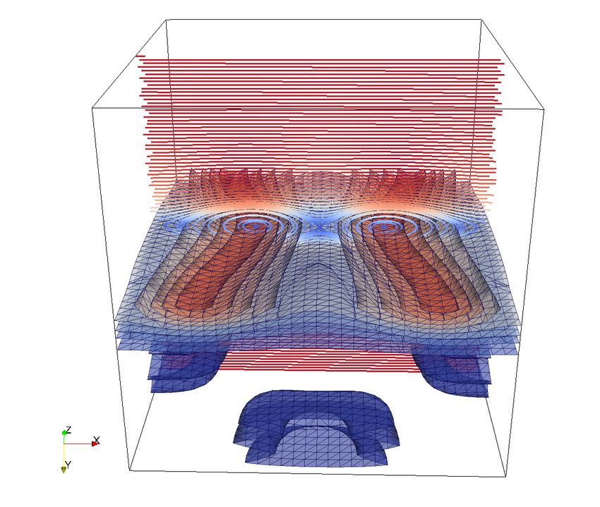
ETNA
                                                                        Kent State University and
                                                                     Johann Radon Institute (RICAM)

366             P. OHM, T. WIESNER, E. CYR, J. HU, J. SHADID, AND R. TUMINARO

factorizations, which manipulate the constituent Jacobian blocks and use inner solvers on
simpler problems. We instead focus on monolithic AMG but still consider blocking ideas when
developing the multigrid components. While a monolithic approach applies AMG directly
to the entire linear system (as opposed to applying multigrid to sub-linear systems), block-
oriented algorithms can be used to construct AMG components such as the relaxation methods
and the grid transfer operators. In this way, one can leverage existing algorithms and software
developed for simpler sub-systems that can then be combined or composed together to address
more complex problems. In fact, it is possible to construct a monolithic multigrid method
even when different grids are used for separate components. Given the problem-dependent
nature of different multiphysics systems, one may need to consider different blocking schemes
for different PDE systems, and so it is essential that solvers provide flexible mechanisms for
defining and manipulating blocks in order to tailor the AMG strategy to specific situations.
     We demonstrate the importance of a flexible blocking scheme in the context of solving
difficult linear systems associated with resistive magnetohydrodynamics (MHD). The gov-
erning partial differential equations consist of conservation of mass, momentum, and energy
augmented by the low-frequency Maxwell’s equations and are often highly ill-conditioned [9,
25, 32, 47, 48]. Depending on the particular MHD scenario, different solver adaptations might
be appropriate. Specifically, we highlight blocking AMG ideas using the MueLu package [3, 4]
(found within Trilinos [29]), which facilitates different block strategies. In one case, a special
block ILU relaxation method is devised that has significant computational advantages over a
more black-box relaxation technique. Here, an ILU factorization is applied separately to the
Navier-Stokes block and to the magnetics block as opposed to applying the ILU factorization
to the entire system. This effectively ignores the coupling between the Navier-Stokes and the
magnetics equations during the incomplete factorization, which leads to a significant reduction
in the time required to actually perform the ILU factorization. The overall monolithic smoother
couples the physics together with a Gauss-Seidel iteration. In another case, we show how
to adapt the solver to address situations where different finite element basis functions are
used to represent the different physical fields of the MHD system. Specifically, one AMG
algorithm is applied to a Q2 Navier-Stokes block while another AMG algorithm is applied to
a Q1 magnetics block, and the results of the two invocations are then composed together to
define the interpolation for the entire MHD system. In this case, the blocking choice avoids
a limitation in applying the existing AMG algorithm/software to a PDE system where the
number of degrees of freedom per spatial location is not constant. That is, the blocking allows
us to leverage algorithms and solve problems that could not be previously addressed with
the existing algorithms. In the future, we plan to expand upon the current block strategies
and consider different AMG schemes for pressures, velocities, magnetics, and the magnetics’
Lagrange multipliers. This will allow us to employ more sophisticated interpolation algorithms
for only the pressure and the Lagrange multipliers, where simpler schemes can adversely
affect the convergence rate.
     In Section 2 we introduce the MHD equations and the accompanying discrete systems of
equations. In Section 3 we give an overview of the algebraic multigrid method. We discuss the
implementation of these algebraic multigrid methods to multiphysics PDE systems in a truly
monolithic manner through the use of blocked operators in Section 4. We demonstrate the
numerical and computational performance benefits of this approach for various test problems
and present the results in Section 5. Finally, we end with concluding remarks in Section 6.

    2. The MHD equations. The model of interest for this paper is the 3D resistive iso-
thermal MHD equations including dissipative terms for the momentum and the magnetic
induction equations [25, 48]. This model provides a base-level continuum description of
conducting fluids in the presence of electromagnetic fields and is useful in the context of mod-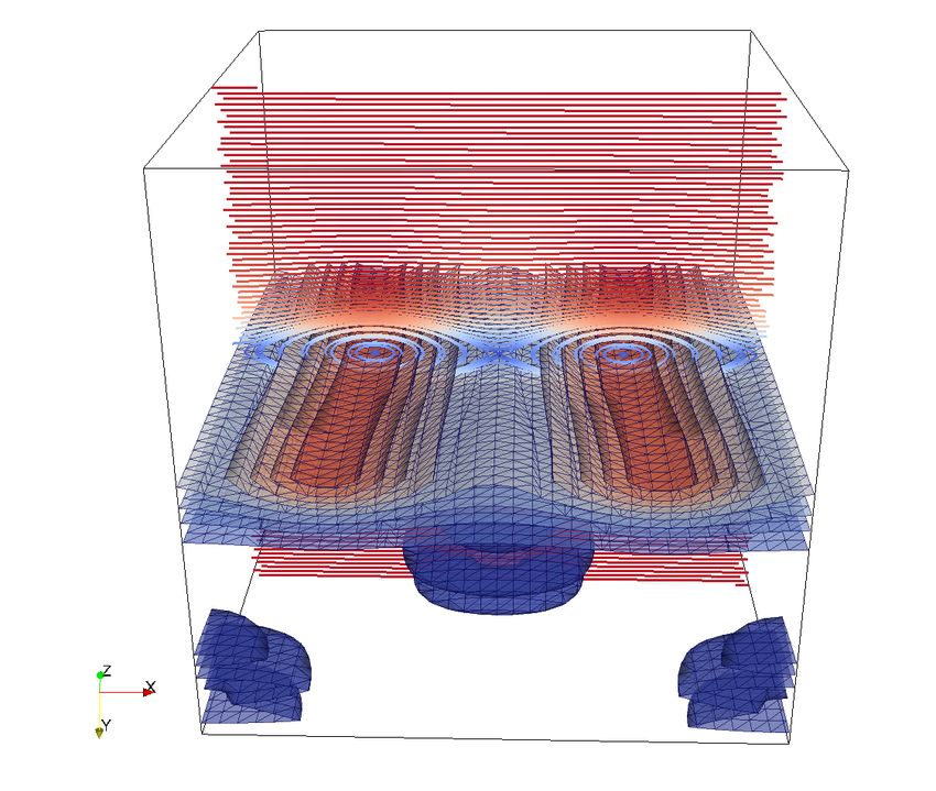
ETNA
                                                                                     Kent State University and
                                                                                  Johann Radon Institute (RICAM)

                       MONOLITHIC AMG FRAMEWORK FOR MULTIPHYSICS SYSTEMS                                     367

                                                   TABLE 2.1
                           Residual form of the governing resistive 3D MHD equations.

         Momentum

                   ∂ρu                 1                1
            rm =       + ∇ · [ρu ⊗ u −    B ⊗ B + (p +     kBk2 )I − µ(∇u + ∇uT )] = 0
                    ∂t                 µ0              2µ0

         Continuity Constraint
                                                           ∂ρ
                                                    rP =      + ∇ · ρu = 0
                                                           ∂t

         Magnetic Induction

                           ∂B                        η
                   rI =       + ∇ · [u ⊗ B − B ⊗ u −     ∇B − (∇B)T + ψI] = 0
                           ∂t                        µ0

         Solenoidal Constraint

                                                       rψ = ∇ · B = 0

eling naturally occurring plasma physics systems (e.g., astrophysics and planetary dynamos)
as well as for technology (e.g., magnetic confinement fusion). The system of equations is
shown in Table 2.1 in residual form. The primitive variables are the velocity vector u, the
hydrodynamic pressure p, the magnetic induction B (hereafter also termed the magnetic field),
and the Lagrange multiplier ψ. The associated plasma current J is obtained from Ampère’s
law as J = µ10 ∇ × B.
     Satisfying the solenoidal involution ∇ · B = 0 in the discrete representation to machine
precision is a topic of considerable interest in both structured and unstructured finite-volume
and unstructured finite-element contexts (see, e.g., [8, 15, 53]). In the formulation discussed
in this study, a scalar Lagrange multiplier (ψ in Table 2.1) is introduced into the induction
equation that enforces the solenoidal involution as a divergence-free constraint for the magnetic
field [2, 8, 10, 11, 15, 48, 53]. This procedure is common in both the finite volume (see, e.g., [8,
15, 53]) and in finite element methods (see, e.g., [10, 11]). We focus on the incompressible
limit of this system, i.e., ∇ · u = 0. This limit is useful to model applications such as
low-Lundquist-number liquid-metal MHD flows [14, 39] and high-Lundquist-number large-
guide-field fusion plasmas [18, 28, 52]. Together, the incompressibility constraint for the fluid
velocity and the solenoid involution for the magnetic field (enforced as a constraint) produce a
dual saddle point structure for the systems of equations [48].
     The spatial discretization is based on the variational multiscale (VMS) finite element (FE)
method [17, 30]. The semi-discretized system is integrated in time with a method-of-lines
approach based on BDF schemes. The weak form of the VMS / stabilized FE formulation for
the resistive MHD equation (see equation (2.1)) is given by

                Z             XZ                                           XZ
(2.1a)     Fhu = wh · rhm dΩ +                     ρτ̂m rhm ⊗ uh : ∇wh dΩ +           τ̂P (∇ · wh )rhP dΩ,
                   Ω                     e    Ωe                             e   Ωe
                Z            XZ
(2.1b)     FPh = q h rhP dΩ +                 ρτ̂m ∇q h · rhm dΩ,
                   Ω             e       Ωe
                Z             XZ                                      XZ
(2.1c)     FhI = Ch · rhI dΩ −   τ̂I (rhI ⊗ uh − uh ⊗ rhI ) : ∇Ch dΩ +   τ̂ψ (∇ · Ch )rhψ dΩ,
                   Ω                 e       Ωe                                          e   Ωe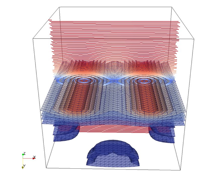
ETNA
Kent State University and
Johann Radon Institute (RICAM)
368 P. OHM, T. WIESNER, E. CYR, J. HU, J. SHADID, AND R. TUMINARO
Z XZ
(2.1d) Fψh = sh rhψ dΩ + τ̂I ∇sh · rhI dΩ,
Ω e Ωe
where τ̂i are the stabilization parameters. Here [wh , q h , Ch , sh ] are the FE weighting functions
for
P the velocity, pressure, magnetic field, and the Lagrange multiplier, respectively. The sum
e indicates that the integrals are taken only over element interiors Ωe and that integration by
parts is not performed. A full development and examination of this formulation is presented
in [48].
2.1. The Block discrete system. A FE discretization of the stabilized equations gives
rise to a system of coupled, nonlinear, non-symmetric algebraic equations, the numerical
solution of which can be very challenging. At each stage of a Newton’s method iteration, the
discrete linearized block system has the following form:
δû
Ju G Z 0 ru
D LP 0 0 δ p̂ rp
(2.2) = − .
Y 0 JI G δ B̂ rI
0 0 GT Lψ δ ψ̂ rψ
Here the block matrix Ju corresponds to the discrete transient, convection, diffusion, and
stress terms acting on the unknowns δû. The matrix G corresponds to the discrete gradient
operator, D corresponds to the discrete representation of the continuity equation terms with
velocity (note for a true incompressible flow this would be the divergence operator denoted as
GT ), the block matrix JI corresponds to the discrete transient, convection, diffusion terms
acting on the magnetic induction, and the matrices LP , Lψ are stabilization Laplacians, which
are described in the next paragraph.
A closer examination of the VMS terms generated by the induction equation and in
the enforcement of the solenoidal constraint through the Lagrange multiplier ψ exhibit the
presence of a weak Laplacian operator acting on the Lagrange multiplier
XZ
Lψ = τ̂I ∇s · ∇ψdΩ.
e Ωe
P R
This term is the analogue of the weak pressure Laplacian LP = e Ωe ρτ̂m ∇Φ · ∇pdΩ
appearing in the total mass continuity equation (see the general discussion for stabilized FE
CFD in [17] and [47, 48] for MHD). These VMS operators are critical in the elimination of
oscillatory modes from the null space of the resistive MHD saddle point system for both (u, p)
and (B, ψ) and allow equal-order interpolation of all the unknowns (see [17] for incompressible
CFD and [2, 10, 11] for resistive MHD). The LP and Lψ operators also help facilitate the
solution of the linear systems with a number of algebraic and domain decomposition-type
preconditioners that rely on non-pivoting ILU factorization, Jacobi relaxation, or Gauss-Seidel
iterations as sub-domain solvers [46, 48, 49].
The difficulty of producing robust and efficient preconditioners for (2.2) has motivated
many different types of decoupled solution methods. Often, transient schemes combine semi-
implicit methods with fractional-step (operator splitting) approaches or use fully-decoupled
solution strategies [1, 26, 27, 31, 33, 35, 41, 43, 44, 51, 54]. In these cases, the motivation is
to reduce memory usage and to produce a simplified equation set for which efficient solution
strategies already exist. Unfortunately, these simplifications place significant limitations on
the broad applicability of these methods. A detailed presentation of the characteristics of
different linear and nonlinear solution strategies is beyond our current scope. Here, we wish to
highlight that our approach of fully coupling the resistive MHD PDEs in the nonlinear solver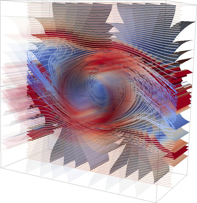
ETNA
Kent State University and
Johann Radon Institute (RICAM)
MONOLITHIC AMG FRAMEWORK FOR MULTIPHYSICS SYSTEMS 369
F IG . 3.1. Multigrid V-cycle algorithm and a graphical representation for a 3-level method.
MGV(u` , b` , `) :
if ` 6= `max
A re
A
p
" (1)
u` ← S`pre (A` , u` , b` )
(0
(0 # po
)
)
A
S
" (1
S0
r` ← b` − A` u`
po
0
st
P1
A
# (2)
u`+1 ← 0 1
R0→
)
→
0
S1
pr
u`+1 ← MGV(u`+1 , R`→`+1 r` , `+1)
e
S1
2 P2
st
R1→
A
→
u` ← u` + P`+1→` u`+1 1
S2
pr
e/
u` ← S`post (A` , u` , b` )
po
st
else
u` ← A−1` b`
preserves the inherently strong coupling of the physics with the goal to produce a more robust
solution methodology [46, 47, 48]. Preservation of this strong coupling, however, places a
significant burden on the linear solution procedure.
3. Multigrid methods. Multigrid methods leverage the fact that many simple iterative
methods can effectively eliminate high-frequency error components relative to the “mesh”
resolution used for discretization. That is, different error components are efficiently reduced
by essentially applying a simple iterative method to the appropriate resolution approximation.
Multigrid methods generally come in two varieties: geometric multigrid (GMG) and
algebraic multigrid (AMG). GMG grid transfers are based on geometric relationships such
as a linear interpolation to transfer coarse solutions to finer meshes. With AMG, coarse-
level information and grid transfers are developed automatically by analyzing the supplied
fine-level discretization matrix. This normally involves a combination of graph heuristics for
coarsening followed by some approximation algorithm to develop operators that accurately
transfer information between the meshes. This paper focuses on AMG as it can be more easily
adapted to complex application domains by non-multigrid scientists.
Figure 3.1 depicts what is referred to as a multigrid V-cycle to solve a linear system
A` u` = b` . Subscripts distinguish between different resolutions. P`+1→` interpolates from
level `+1 to level `. R`→`+1 restricts from level ` to level `+1. A` is the discrete problem on
level `, and for coarse levels it is defined by a Petrov-Galerkin projection
A`+1 = R`→`+1 A` P`+1→` .
S`pre and S`post denote a basic iterative scheme (e.g., a Gauss-Seidel iteration) that is applied to
damp or relax some error components. The overall efficiency is governed by the interplay of
the two main multigrid ingredients: grid transfer operators and the smoothing methods. For a
general overview on multigrid methods, the reader is referred to [7, 55] and the references
therein.
For PDE and multiphysics systems, applying AMG to the entire PDE system (i.e., mono-
lithic multigrid) can be problematic or even impossible for a number of reasons, especially
when the coupling between different solution types (e.g., pressures and velocities) is strong.
Classical simple iterative methods may not necessarily reduce all oscillatory error components
and might even amplify some oscillatory error components. In fact, methods requiring the
inversion of the matrix diagonal (e.g., the Jacobi iteration) are not even well defined when
applied to incompressible fluid discretizations that give rise to zeros on the matrix diagonal.
Further, many standard AMG algorithms for defining grid transfers might lead to transfers
that do not accurately preserve smooth functions. For example, methods such as smoothed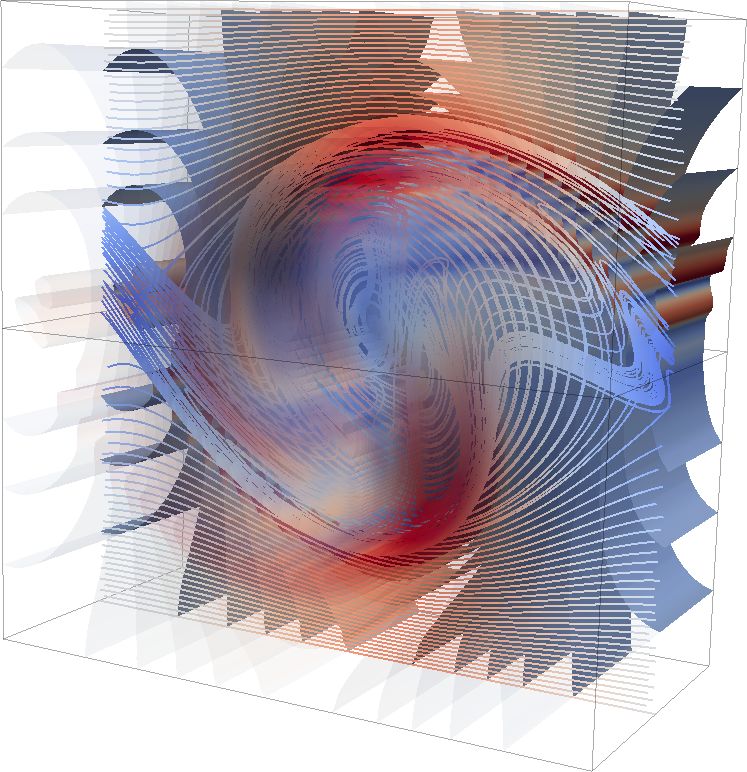
ETNA
Kent State University and
Johann Radon Institute (RICAM)
370 P. OHM, T. WIESNER, E. CYR, J. HU, J. SHADID, AND R. TUMINARO
aggregation rely on a Jacobi-like step to generate smooth grid transfer basis functions. This
Jacobi step, however, will obviously not generate smoother basis functions when the iteration
is not well defined (or when the matrix diagonal is small in a relative sense). The AMG
software itself may not even be applicable to the PDE system when different FE basis func-
tions are used to represent different fields within the system. For PDE systems, most AMG
codes assume that the different equations are discretized in a similar way. In particular, AMG
coarsening algorithms (or for our approach aggregation algorithms) are often applied by first
grouping all degrees of freedom (DoFs) at each mesh node together and then applying the
coarsening algorithms to the graph induced from the block matrix. This has the advantage
that all unknowns at a mesh point are coarsened in the same fashion. However, the approach
breaks down when the number of DoFs associated with different fields varies or if all DoFs
are not co-located, e.g., when using quadratic basis functions to represent velocities while
pressures employ only linear basis functions. In previous versions of our AMG software,
the only alternative to this simple PDE system technique would be to completely ignore the
multiphysics coupling and effectively treat the entire system as if it were a scalar PDE, which
almost always leads to poor convergence.
4. Truly monolithic block multigrid for the MHD equations. In this section we pro-
pose a multigrid method for multiphysics systems that can be represented by block matrices
allowing one to adapt both the relaxation algorithms and the grid transfer construction algo-
rithms to the structure of the system.
4.1. Block matrices and multigrid for PDE systems. As illustrated in the previous
MHD discussion, PDE systems are often represented by block matrices as in, for example,
equation (2.2). More generally, block systems can be written as
A00 A01 · · · A0N x0 b0
A10 A11 · · · A1N x1 b1
(4.1) .. .. = .. ,
.. .. ..
. . . . . .
AN 0 AN 1 ··· AN N xN bN
where each component of the vector xi is a field in the multiphysics PDE and the sub-matrices
Aij are approximations of operators in the governing equations.
One preconditioning approach to PDE systems follows a so-called physics-based strategy
(see Figure 4.1a). These techniques can be viewed as approximate block factorizations
(involving Schur complement approximations) to the block matrix equations (4.1). The
Schur complement arises naturally during a block LU factorization of a linear system, in
which the block upper triangular factor has a block diagonal entry referred to as the Schur
complement. The exact Schur complement involves a matrix inverse, which is not feasible
for large sparse systems. In such cases, the inverse is typically approximated, e.g., with
the application of an iterative solve. More detailed information can be found, for example,
in [60]. The factorizations are usually constructed based on the underlying physics. Here,
different AMG V-cycle sweeps are used to approximate the different sub-matrix inverses that
appear within the approximate block factors. As the sub-matrices correspond to single physics
or scalar PDE operators, application-specific modifications to the multigrid algorithm are
often not necessary. This makes the physics-based strategy particularly easy to implement as
one can leverage ready-to-use multigrid packages. Several methods that follow this popular
strategy are described in [21] and the references therein. While the physics-based approach
has some practical advantages, the efficiency of the preconditioner relies heavily on how
well the coupling between different equations within the PDE is approximated by the block
factorization.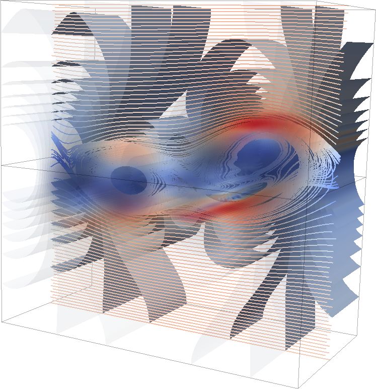
ETNA
                                                                                       Kent State University and
                                                                                    Johann Radon Institute (RICAM)

                  MONOLITHIC AMG FRAMEWORK FOR MULTIPHYSICS SYSTEMS                                            371

    In this paper, we instead consider a monolithic multigrid alternative to a physics-based
approach. A monolithic scheme applies a multigrid algorithm to the entire block PDE
system, and so the AMG scheme effectively develops a hierarchy of block PDE matrices
associated with different resolutions. Figure 4.1 contrasts the two approaches and highlights
the monolithic approach’s key potential advantage, namely an explicit representation of the
cross-coupling defined by A01 and A10 on all multigrid hierarchy levels. In contrast, a physics-

                   F IG . 4.1. Two multigrid approaches to address multiphysics applications.

                                                                                               1
                                                                                           0
                                                                                    A
                             0
                             1
                         A

                                                                             0

                                                                                                           1
                                                                            0

                                                                                                          1
                                                                        A

                                                                                                    A
                     0

                                       1

                                                                                          )
                   0

                                     1

                                                                                    A A (1
               A

                                 A

                                                                                          1 01
                                                                                           0
                                                                           0 1)

                                                                                                    1 1)
                             1

                                                                           A(

                                                                                                    A(
                             0

                                                                            0

                                                                                                     1
                         A
                0 1)

                                    1 1)
                A(

                                    A(

                                     1
                 0

                                                                                        1011))
                                                                                             2
                                                                                       AA ((

                                                                                         0
                                                                             0 2)

                                                                                                   1 2)
                                                                             A(

                                                                                                   A(
                                                                              0

                                                                                                    1
                 0 2)
                 A(

                  0

                                                                                         1 1 )
                                                                                        0 3) 2
                                                                                             (
                                                                                            0
                                                                                       A (A
                                                                                0 3)

                                                                                                 1 3)
                                                                                A(

                                                                                                 A(
                                                                                 0

                                                                                                  1
                  0 3)

                                                                                        1 3)
                  A(

                   0

                                                                                        A(

                                                                                         0
  (a) Physics-based approach with multiple multigrid      (b) Monolithic multigrid with PDE coupling repre-
  approximations to the sub-matrix inverses within an     sented on all multigrid levels.
  approximate block factorization. Example with 4 and
  2 multigrid levels for A00 and A11 .

based scheme must represent the coupling by developing an effective Schur complement
(whose inverse might then be approximated via multigrid sweeps), which can be non-trivial
for complex applications. This is because AMG is only applied to sub-components of the
entire block system within a physics-based scheme, and hence cross-coupling terms are not
explicitly projected to coarser levels. On the other hand, a monolithic approach introduces its
own set of application-specific mathematical challenges such as the construction of relaxation
procedures for monolithic systems and the development of coarsening schemes for different
fields within a multiphysics system. The design of efficient multiphysics preconditioners often
requires one to make use of the specific knowledge about the block structure, the mathematical
models of the underlying physics, and the problem-specific coupling of the equations. The
mathematical challenges of multiphysics systems are often further compounded by non-trivial
software challenges. Unfortunately, most AMG packages cannot be customized to particular
multi-physics scenarios without having an in-depth knowledge of the AMG software.
     In the next sections, we propose a monolithic algorithm for the MHD equations that can be
easily adapted and customized using the MueLu package within the Trilinos framework [3, 4].
Though we focus on a concrete MHD case, we emphasize the importance of the software’s
generality in enabling a monolithic approach for those with limited knowledge of the multigrid
package internals.
     4.2. Algebraic representation of the MHD problem. In adapting a monolithic multi-
grid strategy to the MHD equations, a natural approach would be to interpret the system (2.2)
as a 2 × 2 block system where the Navier-Stokes equations are separated from the Maxwell
equations. That is, we treat the Navier-Stokes part and the Maxwell part as separate entities
that are coupled by the off-diagonal blocks as shown in the 2 × 2 block representation of
Figure 4.2. In this way, we can leverage existing ideas/solvers for the Navier-Stokes equations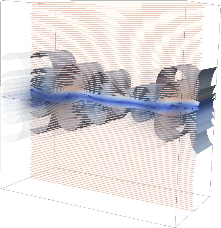
ETNA
Kent State University and
Johann Radon Institute (RICAM)
372 P. OHM, T. WIESNER, E. CYR, J. HU, J. SHADID, AND R. TUMINARO
F IG . 4.2. Representation of the MHD system (2.2) as a 2 × 2 block system.
Ju G Z
δû
D L
ru
δ p̂
P
= − rp
δ B̂ rI
Y JI G
δ ψ̂ rψ
GT Lψ
and for the Maxwell equations. In making this 2 × 2 decomposition, we are effectively em-
phasizing the significance of the coupling between fields within the Navier-Stokes block and
within the Maxwell block as compared to the coupling between Navier-Stokes unknowns and
Maxwell unknowns. This is due to the importance of the coupling constraint equations (e.g.,
incompressibility conditions involving velocities or contact constraints [58]) to the associated
evolution equations. These constraint equations often give rise to saddle-point-like block
systems. Of course, there are physical situations where the coupling between the Navier-Stokes
equations and the Maxwell equations is quite significant, and so a block 2 × 2 decomposition
might be less appropriate. There might also be situations where coupling relationships are
more complex. If, for example, the MHD equations are embedded in another larger more
complex multiphysics problem, then one might need to consider a hierarchy of coupling
configurations, which might require different arrangements/blockings of multigrid ingredients.
Given the problem-specific nature of multiphysics preconditioning, our emphasis here is on
the importance of a flexible software framework to facilitate different types of blocking within
the preconditioner.
For the remainder of the paper the block notation
A00 A01 x0 b
(4.2) =− 0
A10 A11 x1 b1
is used to represent the corresponding blocks from Figure 4.2. The velocity and pressure
increments δû and δp̂ are grouped in x0 , and the Maxwell information is represented by x1 .
In a similar way, the block notation for the residual vector is adopted.
4.3. Monolithic multigrid ingredients for volume-coupled problems. The multiphys-
ics solver that we propose is generally applicable to volume-coupled problems. Volume
coupled means that the different physics blocks are defined on the same domain. Volume-
coupled examples include thermo-structure-interaction (TSI) problems (see [13]) or in our
case the MHD equations. Specifically, within our MHD formulation, all physics equations
(i.e., Navier-Stokes and Maxwell parts) are defined throughout the entire domain. This is in
contrast to interface-coupled problems such as fluid-structure interaction (FSI) applications
(see [16, 24, 34, 37]) or structural contact problems (see [58, 59]), where different equation
sets are valid over distinct domains that are only coupled through a common interface. From a
multigrid perspective, special interface coarsening methods are necessary for interface-coupled
applications, which is not the focus of this paper.
Two multigrid ingredients must be specified to fully define the monolithic solver: the
inter-grid transfer operators and the relaxation or smoother procedures.
4.3.1. Inter-grid transfers for the MHD system. Following the 2 × 2 decomposition
of the MHD system from equation (4.2), we consider rectangular block diagonal inter-gridETNA
Kent State University and
Johann Radon Institute (RICAM)
MONOLITHIC AMG FRAMEWORK FOR MULTIPHYSICS SYSTEMS 373
transfer operators
R00 P00
Ri→i+1 = and Pi+1→i =
R11 P11
for the restriction and prolongation between multigrid levels, respectively. The basic idea uses
the MueLu multigrid package to produce grid transfers for the Navier-Stokes equations and
the Maxwell equations and then leverages MueLu’s flexibility to combine these grid transfer
operators into a composite block diagonal operator.
The block perspective allows us first to build individual components (e.g., P00 and P11 )
with completely separate invocations of MueLu and then combine or compose them together.
As discussed earlier, we rely on underlying core AMG kernels that are applicable to either a
scalar PDE or a PDE system with co-located unknowns. Mixed finite element schemes may
not normally satisfy this co-located requirement, so the ability to separately invoke these core
components to produce P00 and P11 alleviates this restriction, allowing us to apply monolithic
AMG to a wider class of PDE systems. That is, a mixed basis function discretization can
be approached without having to erroneously treat the entire system as a scalar PDE. We
demonstrate this capability at the end of Section 5 through a mixed formulation utilizing
Q2/Q2 VMS for the Navier-Stokes degrees of freedom and Q1/Q1 VMS for the Maxwell
degrees of freedom.
In the case where the unknowns between blocks are co-located (e.g., Q1/Q1 VMS for
both the Navier-Stokes and Maxwell system), we have the option to correlate the grid transfer
construction by having the multigrid invocations share the same aggregates (or coarsening
definition) as depicted in Figure 4.3. In this way, we guarantee that there is a one-to-one
relationship of the coarse Maxwell degrees of freedoms and the associated Navier-Stokes
degrees of freedom. That is, we obtain the same coarsening rate for both, and so the ratio
between Navier-Stokes and Maxwell degrees of freedom is constant on all multigrid levels. It
should be noted that this is relatively straightforward when all equations are defined on the
same mesh using a first-order nodal finite element discretization method. Thus, there are 8
degrees of freedom at each mesh node (four associated with the fluid flow and four associated
with electromagnetics).
Our approach uses aggregation-based multigrid. In contrast to classic multigrid, in which
a subset of fine-level unknowns are selected as coarse-grid unknowns, aggregation-based
approaches group fine-level unknowns into aggregates that form the coarse-grid unknowns.
Specifically, mesh vertices on a given level are assigned to aggregates Ai` such that
N`+1
[
Ai` = {1, ..., N` } , Ai` ∩ Aj` = ∅, 1 ≤ i < j ≤ N`+1 ,
i=1
where N` denotes the number of mesh vertices on level `. Each aggregate Ai` on level ` gives
rise to one node on level `+1. The Ai` are formed by applying greedy algorithms to the graph
associated with a matrix discretization. Specifically, an unaggregated unknown that has no
direct connections via the matrix graph to unknowns already in an existing aggregate is chosen
as an aggregate root. Unknowns that are directly connected to the root via the matrix graph
are grouped with the root to form an aggregate. There are a number of heuristics that may
be used to ignore certain graph connections, based on an analysis involving matrix entries.
Such heuristics are necessary for handling anisotropies in the PDE and/or the underlying mesh.
After the initial greedy sweep phase to assign unknowns to aggregates, there are later phases
that place all remaining unassigned unknowns into existing and/or new aggregates. Typically,
one wants aggregates to be approximately the same size and roughly spherical in shape (forETNA
Kent State University and
Johann Radon Institute (RICAM)
374 P. OHM, T. WIESNER, E. CYR, J. HU, J. SHADID, AND R. TUMINARO
isotropic problems). Piecewise-constant interpolation can then be defined over each aggregate
for each solution component.
Within the current approach, we first build aggregates using the matrix graph of the
sub-block A00 on level i as input. Next, we build separate aggregates based on the graph of
the sub-block A11 or instead clone the Navier-Stokes aggregates when degrees of freedom are
co-located as depicted in Figure 4.3.
F IG . 4.3. Cloned aggregation strategy for volume-coupled multiphysics problems.
Cloned aggregates for
Maxwell equations.
Aggregates built from
Navier-Stokes equations.
Node discretization of cur-
rent level.
As discussed later, this type of multigrid adaptation is relatively straightforward with
MueLu using an XML input file. While cloning is often not essential for many problems, our
plan is to enhance the cloning capability for mixed finite element systems where unknowns
between blocks are not co-located. This enhancement would allow for some correlation
between the aggregates of the different blocks, though they will no longer be identical. We
have found that correlated-aggregation can help avoid stability issues that might arise with the
AMG-generated coarse discretizations when the finest-level discrete operator corresponds to a
saddle point system that does not employ stabilized finite elements. In addition to consistently
coarsening both fluid and electromagnetic variables, the reuse or cloning of aggregates saves a
modest amount of time within the multigrid setup phase. Additional reductions in the setup
cost can be achieved if one defines R11 = R00 and P11 = P00 . Again, this is relatively easy to
do within the MueLu framework, though not necessary. In our experiments, piecewise constant
interpolation is the basis for all grid transfers. This simple grid transfer choice is more robust
for highly convective flows.
4.3.2. Block smoother for the MHD system. A block Gauss-Seidel (BGS) iteration
forms the basis of the multigrid smoother using the notion of blocks already introduced via
the 2 × 2 decomposition. A standard block Gauss-Seidel iteration would solve for an entire
block of unknowns simultaneously, recompute residuals, and then solve for the other block of
equations simultaneously. This corresponds to alternating between a Navier-Stokes sub-block
solve and a Maxwell sub-block solve while performing residual updates after each sub-solve.
Effectively, the 2 × 2 block perspective emphasizes the coupling within the Navier-Stokes
block and within the Maxwell part as each of these blocks correspond to a saddle point system
due to the presence of constraint equations. That is, the difficulties associated with saddle point
systems will be addressed by an approximate sub-block solve. Further, the block Gauss-Seidel
iteration considers the Navier-Stokes block and the Maxwell block equally important as the
iteration simply alternates equally between the two sub-solves. As the exact solution of eachETNA
Kent State University and
Johann Radon Institute (RICAM)
MONOLITHIC AMG FRAMEWORK FOR MULTIPHYSICS SYSTEMS 375
sub-system is computationally expensive, an additive Schwarz domain decomposition (DD)
method with an ILU(0) solve on each domain is used to generate approximate sub-solutions,
associating one domain with each computing core.
While not necessarily an optimal smoother, we have found that ILU(0) is often effective
for the saddle point systems associated with incompressible flow. While additive Schwarz
DD with ILU(0) could be applied to the entire 2 × 2 matrix, this involves significantly more
computation and memory during the setup and apply phases of the smoother. This more
expensive process is generally not needed as the coupling between the block sub-systems is
often much less important than the coupling within the sub-blocks, though there could be
MHD situations with significant cross-coupling between the Navier-Stokes and Maxwell part
that would warrant the smoother applied to the whole system.
Algorithm 1 Damped blocked Gauss-Seidel smoother.
Require: A, b, ω, #sweeps
1: Set initial guess: x := 0
2: for s = 0, s < #sweeps do
3: % Calculate update for Navier-Stokes part
4: Calculate residual: r0 := b0 − A00 x0 − A01 x1
5: Solve approximately A00 x f0 = r0 for x
f0
6: Update intermediate solution: x0 := x0 + ω x
f0
7: % Calculate update for Maxwell part
8: Calculate residual: r1 := b1 − A10 x0 − A11 x1
9: Solve approximately A11 x f1 = r1 for x
f1
10: Update intermediate solution: x1 := x1 + ω x
f1
11: end for
x0
12: return x :=
x1
Algorithm 1 shows the outline of the damped Gauss-Seidel block smoothing algorithm.
First, an approximate solution update x f0 of the Navier-Stokes part is built in line 5 of Algo-
rithm 1 and then scaled by a damping parameter ω in line 6. Similarly, an approximate solution
update xf1 is built for the Maxwell part and scaled by the same damping parameter ω in lines 9
and 10. Please note, that the residual calculation in line 8 employs the intermediate solution
update from line 6. Similarly, an intermediate solution is used for the residual calculation in
line 4 if we apply more than one sweep with the block Gauss-Seidel smoothing algorithm.
As one can see from Algorithm 1, we only need approximate inverses of the diagonal
blocks A00 and A11 . A flexible implementation allows one to choose appropriate local smooth-
ing methods to approximately invert the blocks A00 and A11 . The coupling is guaranteed by
the off-diagonal blocks A01 and A10 in the residual calculations in lines 4 and 8.
4.4. Software. Though this paper demonstrates the multigrid approach for certain MHD
formulations, it is clear that the concept is more general. Due to the problem-dependent nature
of preconditioning multiphysics problems, it is logical to provide a general software framework
that helps design application-specific preconditioning methods. The proposed methods in
this paper are implemented using the next-generation multigrid framework MueLu from the
Trilinos software libraries. In contrast to other publications like [56], which share the same core
idea of a general software framework, MueLu is publicly available through the Trilinos library.
Furthermore, it is fully embedded in the Trilinos software stack and has full native access to all
features provided by the other Trilinos packages. It aims at next-generation HPC platformsETNA
Kent State University and
Johann Radon Institute (RICAM)
376 P. OHM, T. WIESNER, E. CYR, J. HU, J. SHADID, AND R. TUMINARO
and automatically benefits from all performance improvements in the underlying core linear
algebra packages. The core design concept of MueLu is based on building blocks that can
be combined to construct complex preconditioner layouts. Each building block processes
certain input data and produces output data which serves as input for the downstream building
blocks. The relations between the building blocks are easy to modify via an XML input
file. For application-specific adaptions it is usually sufficient to replace specific algorithmic
components while the majority of building blocks can be reused.
5. Experimental results. All simulations were run on a multi-node cluster composed of
nodes with dual 16 core sockets with Intel Broadwell E5-2695 (2.1 GHz) processors. Each
node contains 128 GB RAM, and network communication is performed on an Intel Omni-Path
high-speed interconnect.
5.1. The MHD generator. This problem is a steady-state MHD duct flow configuration
representing an idealized MHD generator, where an electrical current is induced by pumping a
conducting fluid (mechanical work) through an externally applied vertical magnetic field [48].
The bending of the magnetic field lines produces a horizontal electrical current. The geometric
domain for this problem is a square cross-sectional duct of dimensions [0, 15] × [0, 1] × [0, 1].
The velocity boundary conditions are set with Dirichlet inlet velocity of u = (u, 0, 0), no-slip
conditions on the top, bottom, and sides of the channel and natural boundary conditions on the
outflow. The magnetic field on the top and bottom boundaries is specified as B = (0, Bygen , 0),
where
1
x − x x − x
on off
Bygen = B0 tanh − tanh .
2 δ δ
Here, B0 is the strength of the field, and δ is a measure of the transition length-scale for the
application of the field. The inlet, outlet, and sides are perfect conductors with B · n̂ = 0
and E × n̂ = 0, where n̂ is the outward facing unit normal vector. Zero Dirichlet boundary
conditions are applied on all surfaces for the Lagrange multiplier. The problem is defined
by three non-dimensional parameters: the Reynolds number Re = ρuL/µ, the magnetic
√
Reynolds number Rem = µ0 uL/η, and the Hartmann number Ha = B0 L/ ρνη. Here, u is
the maximum x-direction velocity. The parameters in this problem are taken to be u = 1.0,
ρ = 1, B0 = 3.354, µ0 = 1, η = 1, xon = 4.0, xoff = 6.0, and δ = 0.5. At each stage of the
Newton method, a non-restarted GMRES iterative Krylov solver is used. The convergence
criteria for each of the linear solves is taken as a relative residual reduction of 10−3 , which is
consistent with an inexact Newton-type procedure [19, 20, 50]. The reference preconditioner
is a fully-coupled AMG method (FC-AMG), where the relaxation method, additive Schwarz
DD with overlap one and ILU(0) on each domain, is applied to the entire system that includes
the off-diagonal coupling between the fluids and magnetics (see [38]). For the blocked variant
presented in this manuscript (Section 4), we use BGS as a relaxation method (AMG(BGS)).
The approximate solves for the sub-blocks are handled with additive Schwarz DD with overlap
one and ILU(0) on each domain. The coarse grid for both the FC-AMG and AMG(BGS) is
solved directly.
In the first study, we investigate the number of iterations and solution time as a function
of the block Gauss-Seidel (BGS) damping parameter ω for various values of the viscosity
µ ∈ {0.006, 0.007, 0.008, 0.01, 0.02, 0.04}, which effectively sets the range for the non-
dimensional parameters: 25 ≤ Re ≤ 167, 17 ≤ Ha ≤ 43, and Rem = 1.
Figure 5.1 displays the accumulated number of linear iterations and solver timings for
the MHD generator problem on a 240 × 16 × 16 mesh using 32 processors. The numbers
on the side of the columns in Figure 5.1a denote the number of nonlinear iterations. TheETNA
Kent State University and
Johann Radon Institute (RICAM)
MONOLITHIC AMG FRAMEWORK FOR MULTIPHYSICS SYSTEMS 377
F IG . 5.1. Solver performance for the AMG(BGS) preconditioner with 1 BGS coupling iteration versus the
fully-coupled FC-AMG preconditioner for the MHD generator example on a 240 × 16 × 16 mesh using 32 processors.
545 581
443
534
600 430
342
399
500 307
385
413 150 93.05
> 600 98.93
516 66.11
400 273 326 317 91.84
349 405 73.82
279 53.19 141.43
Iterations
300
236
260 100 68.25 66.50
247 48.94 73.04
219
193
Time [s]
200 174 374 44.29 56.68 55.25
204 200 45.21 60.74 69.49 88.57
176 42.10
100 126 164 181 230 50 43.92 45.99
156 308 39.65
95 32.44 32.55
117 175
86 139 197 36.88 32.80 36.37
G 106 25.46 64.48
140 33.50
- AM 79 170 231 18.94 30.07 31.13 40.93
FC )) 99 23.94
S (0.2 ) 71 G
17.60 27.07
32.47 53.79
) 36.06
1 BG (0.3 68
92
- AM 16.60
22.03
G( GS )) FC )) 27.07
0.4 0.2
0.
85 20.63
AM 1B S(
31.79 41.51
00
G( S( )) 63 )) 15.40
6
105
BG (0.5 BG (0.3
0.
AM 19.62
00
(1 ) 60 (1 GS ) 14.88
GS .4)
7
G .6) G
0.
0.
B AM B 0
AM 0
00
( 18.57
00
(1 ( 1
y
G( GS ))
6
S )) 14.05
8
it
G 55
G s .5
0.
.7 21.87
0.
co
M B 0
AM 1B (0
00
(
01
A 1
is
G( GS ))
7
G( ))
V
GS 13.65
(0.6
0.
(0.8
0.
AM 1B AM 1B
00
02
y
G( GS ))
8
it
( S )) 13.00
s
G G (0.7
0.
co
0.9
0.
AM 1B AM 1B
01
is
04
S( ( )
V
G( G G S )
BG (0.8
0.
AM AM 1B
02
G (1 G( GS ))
0.9
0.
AM AM 1B
04
G( S(
AM BG
G (1
AM
(a) Accumulated number of linear iterations depend-
ing on the BGS damping parameter and viscosity. (b) Solver timings (setup + iteration phase) depend-
The numbers on the sides of the column denote the ing on the BGS damping parameter and viscosity.
number of nonlinear iterations to solve the system.
number on the z-axis represents the accumulated number of linear iterations. Figure 5.1b
displays the accumulated solver timings (setup and iteration phase) of the corresponding
preconditioning variants. The timings are averaged over 5 simulations. As one can see from
Figure 5.1, the right choice of the BGS damping parameter is crucial for smaller viscosities.
Even though the optimal damping parameter depends on the problem, in practice a damping
parameter ω near 0.5 seems to work well. Figure 5.2 shows the accumulated linear iterations
and the solver times for the MHD generator example on a finer 480 × 32 × 32 mesh using
256 processors. One can see in Figure 5.2a that a higher number of BGS iterations reduces
the overall number of linear iterations, but not enough to compensate for the higher costs per
iteration (see Figure 5.2b). For reference, the fully-coupled approach is also shown in the
back row (labeled as FC-AMG). This option generally takes more time and iterations than the
multiphysics solver, varying somewhere between 2 and 3 times slower. In experiments not
shown here, tightening the linear solver tolerance lead to comparable scalability, albeit with
higher runtime for all preconditioners. As a result we have focused on the looser tolerances to
minimize runtime for these engineering applications.
5.2. The hydromagnetic Kevin-Helmholtz (HMKH) problem. A hydromagnetic Kel-
vin-Helmholtz unstable shear layer problem is a configuration used to study magnetic recon-
nection [48] and is posed in a domain of [0, 4] × [−2, 2] × [0, 2]. It is described by an initial
condition defined by two counter flowing conducting fluid streams with constant velocities
u(x, y > 0, z, 0) = (5, 0, 0) and u(x, y < 0, z, 0) = (−5, 0, 0) and a Harris-sheet-sheared
magnetic field configuration given by B(x, y, z, 0) = (0, B0 tanh(y/δ), 0). The boundary
conditions are periodic on the right and left as well as on the front and back. The top and
bottom are impenetrable for the fluid velocity, and the magnetic field is defined by the Harris
sheet. The magnetic Lagrange multiplier is taken as zero on all boundaries. The parameters
in this problem are ρ = 1, µ0 = 1, µ = 10−4 , η = 10−4 , B0 = 0.3333, δ = 0.1 to produce
√
Re = 5 × 10⁴ , Rem = 5 × 10⁴ , and an Alfven velocity, uA = B0 / ρµ0 = 0.333, resulting
in an Alfvenic Mach number MA = u/uA = 15. For these non-dimensional parameters, theETNA
Kent State University and
Johann Radon Institute (RICAM)
378 P. OHM, T. WIESNER, E. CYR, J. HU, J. SHADID, AND R. TUMINARO
F IG . 5.2. Solver performance for the AMG(BGS) preconditioner with a fixed damping parameter and 1 or
2 BGS coupling iterations versus the fully coupled FC-AMG preconditioner for the MHD generator example on a
480 × 32 × 32 mesh using 256 processors.
3
92
6 95.85
1
4
75
90
6 5 78.36
93.91
0
100
9
76
5
900 100 80.42
1
800
71
5 90
74.26
45.40
2
700 80
35
6 48.48
600 70
Iterations
2
0
0
24
50 60
23
31.02
8
6
44
5 34.44
5 49.10
7
400 50
Time [s]
21
5 29.56
6
16
32.84
3
5
300 40
20
28.11
6
5
15
5 30.15
200 30
1
17
0.
24.57
0
00
14
5 6
5
100 20 26.43
0.
0
15
00
0.
22.32
9
00
11
7
5
6
0.
5 10 24.72
0
0.
08
ty
8
0
10
MG
07
si
0.
co
5
0
0.
-A
is
1
))
V
0
FC
08
ty
0.4
0.
G
si
0
S(
0.
co
AM
2
))
0
is
-
1
G 4 ))
V
.
0.
1B (0 FC 0.4
0
0.
4
G(
0
GS S(
2
AM 2B G 4))
(0.
0.
B
G(
0
1
4
A M G( GS
AM ( 2B
G
AM
(a) Accumulated number of linear iterations depend-
ing on the BGS iterations and viscosity. The numbers (b) Solver timings (setup + iteration phase) depend-
on the sides of the column denote the number of ing on the BGS iterations parameter and viscosity.
nonlinear iterations to solve the system.
shear layer is Kelvin-Helmholtz unstable and forms a vortex sheet that evolves with time and
undergoes thin current sheet formation, vortex rollup, and merging. Figure 5.3 displays the
unstable shear layer evolving from smaller vortices to a larger vortex.
F IG . 5.3. Hydromagnetic KH problem with Re = 5 × 10⁴ , Rem = 5 × 10⁴ , MA = 15. Pressure contour
lines and velocity streamlines.
(a) t = 3.0s. (b) t = 3.5s. (c) t = 4.0s. (d) t = 4.5s.
To study the behavior of the nonlinear- and linear solver, we perform transient simulations
of the problem with CFLmax = 0.25 and CFLmax = 0.5. The step sizes were chosen to
resolve the advected time scale. Below, we compare the timings and number of iterations of
non-restarted GMRES with a solver tolerance of 10−3 for the reference fully-coupled AMG
preconditioner (FC-AMG) and the blocked AMG(BGS) preconditioner.ETNA
Kent State University and
Johann Radon Institute (RICAM)
MONOLITHIC AMG FRAMEWORK FOR MULTIPHYSICS SYSTEMS 379
Figures 5.4 and 5.5 illustrate the solver performance for the different preconditioning
strategies over a time sequence for the HMKH problem with a maximum CFL number of 0.25
and 0.5, respectively. We ran the problem both on a 64 × 32 × 16 mesh on 32 processors and
a 128 × 64 × 32 mesh on 256 processors. Generally, the FC-AMG method needs the least
number of iterations, whereas the blocked AMG(BGS) variant with only 1 coupling iteration
needs the highest number of iterations. Increasing the number of BGS coupling iterations
reduces the number of linear iterations getting closer to the reference method. However,
looking at the linear solver time (setup and iteration phase), we see the opposite picture. The
FC-AMG method is the slowest, and the blocked AMG(1 BGS) is the most time-efficient
method. Comparing the solver behavior for the different meshes, there is a slight increase in
the linear iteration count for the finer meshes. So, while the weak scaling is not optimal, the
iteration growth with problem size is mild.
F IG . 5.4. HMKH example (CFLmax = 0.25). The left plots show the accumulated linear iterations over time
steps. The right plots show the accumulated solution time (setup + iteration phase) per time step.
40 Accumulated timings per timestep [s]
Accumulated lin. it. per timestep [·]
FC-AMG FC-AMG
AMG(1 BGS (0.4, ILU)) AMG(1 BGS (0.4, ILU))
AMG(2 BGS (0.4, ILU)) AMG(2 BGS (0.4, ILU))
30
10
20
5
10
0 0
500 1,000 1,500 2,000 2,500 3,000 500 1,000 1,500 2,000 2,500 3,000
Timesteps Timesteps
(a) 64 × 32 × 16 mesh, ∆t = 0.0015625s, 32 processors.
60
Accumulated timings per timestep [s]
20
Accumulated lin. it. per timestep [·]
FC-AMG FC-AMG
AMG(1 BGS (0.4, ILU)) AMG(1 BGS (0.4, ILU))
AMG(2 BGS (0.4, ILU)) AMG(2 BGS (0.4, ILU))
15
40
10
20
5
0 0
0 1,000 2,000 3,000 4,000 5,000 0 1,000 2,000 3,000 4,000 5,000
Timesteps Timesteps
(b) 128 × 64 × 32 mesh, ∆t = 0.00078125s, 256 processors.
Numerical results are further summarized in Tables 5.1 and 5.2. The first column denotes
the average number of nonlinear iterations per time step for the full simulation. One can see
that the number of BGS coupling iterations has some influence on the nonlinear solver, even
though there is no clear trend. The second column represents the average number of linear
iterations per nonlinear iteration. As one would expect, a higher number of BGS coupling
iterations reduces the number of linear iterations necessary to solve the problem. The nextETNA
Kent State University and
Johann Radon Institute (RICAM)
380 P. OHM, T. WIESNER, E. CYR, J. HU, J. SHADID, AND R. TUMINARO
F IG . 5.5. HMKH example (CFLmax = 0.5). The left plots show the accumulated linear iterations over time
steps. The right plots show the accumulated solution time (setup + iteration phase) per time step.
40
Accumulated timings per timestep [s]
15
Accumulated lin. it. per timestep [·]
FC-AMG FC-AMG
AMG(1 BGS (0.4, ILU)) AMG(1 BGS (0.4, ILU))
AMG(2 BGS (0.4, ILU)) AMG(2 BGS (0.4, ILU))
30
10
20
5
10
0 0
200 400 600 800 1,000 1,200 1,400 1,600 200 400 600 800 1,000 1,200 1,400 1,600
Timesteps Timesteps
(a) 64 × 32 × 16 mesh, ∆t = 0.003125s, 32 processors.
60
Accumulated timings per timestep [s]
20
Accumulated lin. it. per timestep [·]
FC-AMG FC-AMG
AMG(1 BGS (0.4, ILU)) AMG(1 BGS (0.4, ILU))
AMG(2 BGS (0.4, ILU)) AMG(2 BGS (0.4, ILU))
15
40
10
20
5
0 0
500 1,000 1,500 2,000 2,500 3,000 500 1,000 1,500 2,000 2,500 3,000
Timesteps Timesteps
(b) 128 × 64 × 32 mesh, ∆t = 0.0015625s, 256 processors.
three columns give the average setup time, the average solve time, and the average overall time
for the linear solver per nonlinear iteration. The AMG(BGS) variants have a clear advantage in
the setup costs, but the iteration costs are higher. That is, fully-coupled AMG using an additive
Schwarz method with ILU(0) that includes Navier-Stokes and Maxwell coupling provides
some convergence benefits, but at the cost of a very large setup time. The last three columns
show the absolute setup, solve, and overall solver time for finishing the simulation. It should be
noted that the FC-AMG method is generally more competitive with the block-oriented solvers
for this problem, and it can even modestly outperform some of the block-oriented variants.
That is, a block approach to monolithic AMG often yields a faster method than a traditional
(non-block) AMG strategy, but certainly not all of the time. More generally, a block-oriented
approach provides additional algorithm possibilities to address complex multiphysics problems
by combining existing algorithms for the components. These block algorithms can be critical
for some discrete systems (such as the mixed finite element system shown in Section 5.4) or
provide significant gains for other systems such as those shown in Figure 5.2. In still other
cases, such as those in Figure 5.5, the gains may be more modest.
5.3. Island coalescence. The island coalescence problem is a prototype problem used to
study magnetic reconnection. While seemingly dominated by transient dynamics, a scalable
simulation of this problem requires correctly handling the bidirectional coupling between the
fluid and the magnetics equations. This is evident from the larger Alfven wave CFLs used inETNA
Kent State University and
Johann Radon Institute (RICAM)
MONOLITHIC AMG FRAMEWORK FOR MULTIPHYSICS SYSTEMS 381
TABLE 5.1
HMKH problem for CFLmax = 0.25.
nT Number of time steps
nN Accumulated number of all nonlinear iterations
n Accumulated number of all linear iterations
Legend: L
tSe Multigrid setup time
tSo Multigrid solution time (iteration phase)
tΣ Solver time (setup + iteration phase)
nN nL tSe tSo tΣ
Preconditioner nT nN nN nN nN tSe tSo tΣ
128 × 64 × 32 64 × 32 × 16
FC-AMG 1.47 7.72 3.08 0.68 3.76 14443.59 3186.92 17630.51
AMG(1 BGS (0.4, ILU)) 1.37 10.18 1.46 1.11 2.57 6393.33 4854.98 11248.30
AMG(2 BGS (0.4, ILU)) 1.47 9.25 1.47 1.65 3.12 6909.57 7780.94 14690.51
AMG(3 BGS (0.4, ILU)) 1.49 8.53 1.47 2.14 3.61 7034.32 10238.93 17273.25
FC-AMG 1.53 10.51 3.37 0.99 4.36 28307.94 8318.34 36626.28
AMG(1 BGS (0.4, ILU)) 1.55 13.96 1.75 1.73 3.48 14884.65 14781.09 29665.74
AMG(2 BGS (0.4, ILU)) 1.51 11.87 1.74 2.39 4.13 14484.49 19942.69 34427.18
AMG(3 BGS (0.4, ILU)) 1.42 10.69 1.74 3.07 4.81 13619.80 23986.51 37606.32
TABLE 5.2
HMKH problem for CFLmax = 0.5.
nT Number of time steps
nN Accumulated number of all nonlinear iterations
n Accumulated number of all linear iterations
Legend: L
tSe Multigrid setup time
tSo Multigrid solution time (iteration phase)
tΣ Solver time (setup + iteration phase)
nN nL tSe tSo tΣ
Preconditioner nT nN nN nN nN tSe tSo tΣ
128 × 64 × 32 64 × 32 × 16
FC-AMG 1.81 8.06 3.07 0.70 3.77 8878.08 2013.02 10891.10
AMG(1 BGS (0.4, ILU)) 1.77 11.19 1.47 1.24 2.71 4166.08 3513.20 7679.28
AMG(2 BGS (0.4, ILU)) 1.74 9.39 1.46 1.68 3.14 4081.49 4667.58 8749.07
AMG(3 BGS (0.4, ILU)) 1.75 8.68 1.48 2.20 3.68 4143.28 6192.65 10335.92
FC-AMG 1.94 11.19 3.36 1.06 4.42 20883.40 6616.06 27499.46
AMG(1 BGS (0.4, ILU)) 1.91 15.05 1.74 1.91 3.65 10691.61 11677.32 22368.94
AMG(2 BGS (0.4, ILU)) 1.89 12.74 1.74 2.58 4.32 10572.95 15626.96 26199.91
AMG(3 BGS (0.4, ILU)) 1.80 11.33 1.74 3.19 4.93 10038.69 18408.73 28447.42
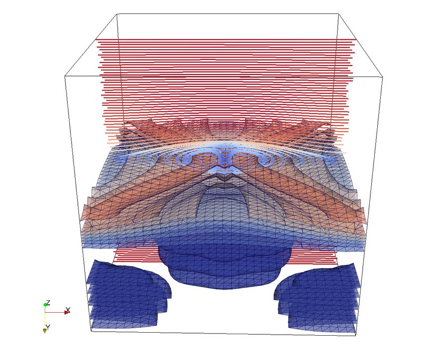
F IG . 5.6. Structure of the current tubes in the 3D island coalescence problem with S = 2 × 10⁴ for the initial
condition and for the times in the evolution of the problem of t = 2, 3, 4. The 3D current tubes have bent in the
z-direction and form current sheets.
(a) t = 0.0s. (b) t = 2.0s. (c) t = 3.0s. (d) t = 4.0s.You can also read