A self consistent probabilistic formulation for inference of interactions - Nature
←
→
Page content transcription
If your browser does not render page correctly, please read the page content below
www.nature.com/scientificreports
OPEN A self‑consistent probabilistic
formulation for inference
of interactions
Jorge Fernandez‑de‑Cossio1*, Jorge Fernandez‑de‑Cossio‑Diaz2 & Yasser Perera‑Negrin3
Large molecular interaction networks are nowadays assembled in biomedical researches along with
important technological advances. Diverse interaction measures, for which input solely consisting of
the incidence of causal-factors, with the corresponding outcome of an inquired effect, are formulated
without an obvious mathematical unity. Consequently, conceptual and practical ambivalences arise.
We identify here a probabilistic requirement consistent with that input, and find, by the rules of
probability theory, that it leads to a model multiplicative in the complement of the effect. Important
practical properties are revealed along these theoretical derivations, that has not been noticed before.
A combination of drugs can produce synergistic effects even when administered separately in time. The first can
“prepare the field” for the later action of the second, without meeting in a direct physical contact. This meaning
of interaction has been practical in toxicology for the discovery of dosage combinations that better perform
on clinical parameters of interest. A similar notion is in usage in epidemiology and in the construction of gene
interactions networks.
Forefront high-throughput technologies are delivering interaction data relevant for the study of poorly known
complex systems, like the cell. Factors and effects are often the sole kind of data released in large scale experiments
by these technologies. For example, synthetic genetic arrays and gene-editing technologies, in both targeted and
large-scale experiments, allows to knock out or selectively activate/repress target genes along the genome in
various cell types and organisms, altering cellular process and f unctions1,2. These factors need not be in direct
physical contact, while the observable effect, measured in terms of a particular biological outcome, laid far at
the other end of the triggered process. The mechanisms and process structures operating in the way from factors
and their effect are not observable at this experimental stage. The tacit assumption is that recurrent patterns of
factor and effect provide information of the presence of cross-talk structures along the process perturbed by the
factors (ambient, genes, drugs, …), in their way to the outcome of some measurable parameter (disease, blood
pressure, live expectancy, cellular growth rate, fitness, transcript expression, or any other biological activity/
phenotype). The above loose meaning of interaction fits to the kind of inference permitted by this kind of data,
the circumstance that we focus in this manuscript.
The data in these large scale screening provide no cues of when, where and how the intermediate events
interconnect3. Later enrichments with functional annotations and additional biological knowledge permit the
systematic elucidation of higher-level principles of the cellular organization and function. The utility of theses
mapping efforts has been shown across diverse prokaryotes and eukaryotes organisms including mammalian
and human cells1,4–6. Therefore, inaccuracy at the interaction mapping stage propagates to the subsequence stages
of enrichment and functional m apping7.
However, at the basic level, the definition of interaction remains conceptually ambivalent. The issue is not new,
testimonies of everlasting debates can be traced back along more than a c entury8. Currently, diverse measures
are advocated in the literature, and the concept of interaction await open for resolution.
On one side, interaction models in epidemiology gravitates around risk, i.e. the probability of a disease (effect)
given the exposure factors (radiations, smoking, diet, pollution, genes, etc.). Dominant theoretical and methodo-
logical streams advocate developments from causal inference (ex. counterfactuals, potential outcomes, sufficient
cause), not without controversies among scholars and philosophers9–12. Some epidemiologist proclaim that
there is no biological rationale for calling interactions to the product terms in a regression model, arguing that
they can disappear or even change sign by transforming the outcome scale (ex. logarithm)13,14. Others are more
1
Bioinformatics Department, Center for Genetic Engineering and Biotechnology (CIGB), PO Box 6162,
CP10600 Havana, Cuba. 2Systems Biology Department, Center of Molecular Immunology, PO Box 6162,
CP10600 Havana, Cuba. 3Molecular Oncology Group, Pharmaceutical Division, Center for Genetic Engineering and
Biotechnology (CIGB), PO Box 6162, CP10600 Havana, Cuba. *email: jorge.cossio@cigb.edu.cu
Scientific Reports | (2020) 10:21435 | https://doi.org/10.1038/s41598-020-78496-8 1
Vol.:(0123456789)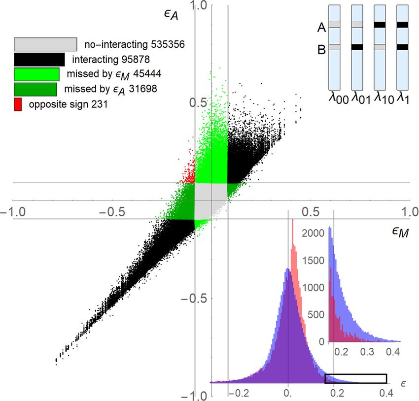
www.nature.com/scientificreports/
confident to cast sufficient-cause interactions method in complementary log regressions framework15. Another
faction claim for broadening the scope of the casual inference school, and for a more pluralistic a pproach11,12.
On another side, ad hoc measures are adopted in the construction of large-scale genetic interaction net-
works. Often, regression model are written down directly in terms of the physical parameters measured in the
experiment (ex. growth rate, fold change, viability, drug inhibition, lethality, etc.), with a hasty explanation for
the rational of the c hoice5,16–19. Based on "genetic" g rounds20, the double-mutant fitness is expected to be the
product of the single-mutant fitness, on absence of interaction, but fitness itself exhibit a plurality of meanings,
or varied in scales. A phenotype can be consistently expressed in terms of any monotonic function (logarithms,
exponential, etc.) of the “original” phenotypic scale. But the product or the addition in one scale is not the same
than in another. Evoking a “regression model” or a “multiplicative model” is just not enough. The concerns is
not new, and the reaction should not be confined to comparisons between mathematically defined measures in
term of ad hoc criteria of performance3,7,19. Of course, performance is the final goal, yet this path of assessment
is limited to the already defined competitors, a useful but postmortem dictamen.
Striving to come out from this conceptual quandary in the direction of fundamental development, we under-
take a pragmatic resolution of the concept of interaction that depart from precedent approach. In this endeavour,
we do not write down in advance a mathematical definition of interaction, but advocate a concept that comply
with the practical meaning and kind of input data stated above. We identify from a verbally stated definition,
elementary but general probabilistic requirements for multivalued factors and dichotomous effect scenarios.
Sticking to the rules of probability theory, we derive a model which is general and simple. Finally, we illustrate
for a genetic interaction mapping case, how to cast the measured parameters into the language of factor and
effect, so as to apply the framework just derived. Though we do not pose a causal inference approach, we detour
briefly into association and causality in connection with our development.
Motivation
Genetic interactions underlie diverse aspects of biology, including the evolution of sex, speciation, and complex
disease. Simple inbred systems, such as yeast, provide an experimental format for mapping the genetic inter-
actions networks of a cell. Genome-scale interaction studies in isogenic yeast populations, collected growth
measurements from four possible mutant states for each pair of genes A and B (wild-type (00), single-mutants
(01 and 10), and double-mutant (11). A schematic representation is shown in the upper-right of Fig. 1. Genes
A and B are regarded to interact when the growth rate 11 of the double mutant is unexpected from the growth
rates 01 and 10 of the single mutants. This consent is intuitively appealing, but far from guiding to a definite
physical or biological meaning, merely defers the issue to what can be regarded as a reasonable expectation of
the effect in the absence of interaction. Indeed, these studies disagree on what they consider for “unexpected”,
and their derived genetic interaction measures d iffer7.
Mathematical functions delivering the expectation of the combined factor effect, from the individual fac-
tor’s effect, have been named neutrality function7. So far, the mathematical definition of a neutrality function
remain open to arbitrariness3,7,21. Mani et al7 examined properties of four reported definitions of interaction
and show that the choice can dramatically alter the resulting set of genetic interactions with inconsistencies that
propagates to the functional mapping. For a quick illustration of the magnitude of this impact, we compare two
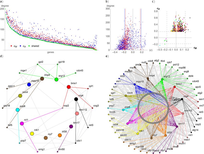
measures at the basic interaction networks level, of a more recent and extensive global genetic interaction studies
in Saccharomyces Cerevisiae1. One of the measures, εM = 11 − 01 10, use a neutrality function that multiply
the single-mutants r ates1, while the other measure, εA = 11 + 1 − 01 − 10, add the single-mutants r ates22.
Figure 1 show the comparison on the Essential x Essential SGA library (See Data Availability). The initial
high correlation between the most extreme negative interactions (lower-left quadrant of the plot), progressively
deteriorate, due to a remarkable propensity of the measure εA to score larger positive interactions with respect
to εM. Overall,
the two measures have
discrepancies in more than 44% of the
pairs reported by one or the other
measure, i.e. #missed + #opposite / #missed + #opposite + #interacting . The superposed histograms in Fig. 1
show the distribution along the magnitude of interaction computed with both measures. A preponderance of
genes with positive interaction obtained with εA are notable in the right tail, by thousands, compared to the
obtained with the measure εM.
The issue is not merely on how large the deviation is, but from what and how we measure the deviation. The
question of “from what?” is quantitatively answered by choosing a neutrality function. The question of “how we
measure the deviation?” is another source of plural inspiration. No fundamental agreement in the answers has
been achieved for neither of these questions. The commonest choices are additivity and multiplicative for the
neutrality function, and arithmetic difference and the ratio for the deviation. In both cases, one choice can be
converted to the other by exponentiation or logarithm. But, asking instead, what conversion is appropriate for
the parameters? introduce no progress at all.
Resolution of the concept of interaction
Definition. Modeling controversies can become endless not because the mathematics, but because dispu-
tants might not be talking about the same thing. To keep away from such ambiguities, we commence by stating
explicitly the definition of interaction we advocate.
Before jumping to write down a quantitative definition, we aim to answer the pragmatic question: what we
want from what we have? The inmediate output of the large scale experiment we are focusing, are not going to
explain by themselves mechanistic bases from the analysis of each factor pair, but are delivering hypotheses from
loose interactions networks, that can be tested by further stages of functional analysis. P hillips3 quotation: “…
the mutations must be interacting with one another, at least in the loose sense that they exist within pathways
Scientific Reports | (2020) 10:21435 | https://doi.org/10.1038/s41598-020-78496-8 2
Vol:.(1234567890)
www.nature.com/scientificreports/

                                  Figure 1.  Diverging performance of two measures applied to the same interaction data. In the middle plot,
                                  genetic interaction for each pair of gene is computed with the measures εM = 11 − 01 10 (X axis), and
                                  εA = 11 + 1 − 01 − 10 (Y axis). The color code corresponds to the bar-chart at the upper left. The parallel
                                  lines indicate the standard deviation limits, 0.083 and 0.092, for εM and εA, respectively. The count of the pairs
                                  per each category is shown in a logarithm scale in the bar-chart. The scheme at the upper right show a typical
                                  four genomes set from where interaction data are obtained for a given pair of genes. Gray and black segment of
                                  the genome denote respectively the wildtype and perturbed variant of the genes A and B. The growth rates of
                                  the corresponding yeast isogenic cultures, 01 and 10 corresponds to the single mutants, and 11 to the double
                                  mutant. The histograms at the bottom right show the distribution along the magnitude of interaction computed
                                  with measures εM (red profile) and εA (blue profile). The inset zooms the tail farther than one standard
                                  deviation toward the right tail.

                                  that both influence the same phenotype”, comply with the pragmatic meaning and the factor-effect kind of input
                                  data we aimed. Slightly re-stated for widening the context, we regard that:
                                      Two factors interact with one another, in the loose sense that they exist within pathways that cross or inter-
                                  connect, altering their individual influence to the same effect.
                                      Figure 2a sketch an unobserved response mechanism (shaded area) perturbed by two observed factors A and
                                  B leading to an effect E . According to the definition adopted, on absence of interaction the succession of events
                                  from each factor to the effect follow independent pathways (Fig. 2b). That is, no events triggered by factor A are
                                  disturbed by events triggered by factor B along the pathways of actions leading to the effect E . A schematic rep-
                                  resentation of interacting factors is shown in Fig. 2c. Any form of crossover or cross-talks between the pathways
                                  is regarded as interaction.
                                      We will show how the definition, verbally stated above, become quantifiable in terms of probabilities rules.

Scientific Reports |   (2020) 10:21435 |               https://doi.org/10.1038/s41598-020-78496-8                                                  3

                                                                                                                                              Vol.:(0123456789)
www.nature.com/scientificreports/
Figure 2. Sketch of the interaction scenarios. A and B are observed factors, Z accounts for unobserved factors
and process, and E is the effect of interest. (a) Schematic representation of our limited information. The shaded
area encloses the unobservable mechanism and background agents. Only factors A and B and the effect are
observable. (b) No-interaction scenario. (c) Interaction scenario (there is a cross-over of the pathways from
factors leading to the effect). (Draw with PowerPoint23).
E E
EA EB EZ
EA EB EZ
EA EB EZ
EA EB EZ EA EB EZ
EA EB EZ
EA EB EZ
EA EB EZ
Table 1. Logical structure EA ∨ EB ∨ EZ of E , used as a proxy representing the unobservable mediating
mechanism that involve no cross-talks. The left column shows the possible combination of realization of the
effect. The right column shows the single possible combination of no realization of the effect.
Mathematical formulation. We are interested in classifying the interaction or non-interaction relation-
ships between two multivalued factors with respect to a distant dichotomous effect. An unstated and unproven
assumption in previous approaches is that it is possible to infer interaction from factor and effect data alone,
without considering details of the internal machinery connecting factors and effect. To prove the validity of
this assumption we introduce, by the symbol Z , all the unobservable associated factors and process acting in
the background that escape from our present scrutiny. Since Z is not accessible to us from the data at reach, the
effect E is not fully determined by factors A and B under our control. A probabilistic framework is required to
account for this uncertainty.
The effect due to the individual exposure to factors A, B and Z can be represented as EA, EB and EZ . In the no
interaction case (Fig. 2b), the effect due to the individual or combined exposure can be represented by the logical
expression E = EA ∨ EB ∨ EZ , where ∨ denotes logical OR. The non-occurrence of an effect or the non-exposure
to a factor, is denoted with an overbar (logical NOT). The effect E is not realized only when no one of EA, EB and
EZ is realized. In other words, the negation of the effect, E , is logically equivalent to EA EB EZ , where concatenation
is used to denotes the logical AND. The other seven combinations (left column of Table 1), are undistinguishably
from the observable E . Our data is only provided in terms of E or E , without discerning between the possible
alternative in which E can be realized (left column Table 1). The logical structure EA ∨ EB ∨ EZ of E is used as
a proxy representing the unobservable mediating mechanism that involve no cross-talks. This proxy is only a
temporary construct that cancels in our derivations below. The unobservables EA, EB , EZ and background Z do
not appear in the final equations, remaining only the observables A, B and E.
Rational requirement. The instances of factor A are denoted by a ∈ A and those of B by b ∈ B. According
to the definition, the no-interaction scenario, sketched in Fig. 2b, satisfy the following rational requirements: (i)
the status of factor B carries no relevant information regarding the outcome EA, provided that the status of factor
A is known; (ii) the status of factor A and the occurrence of effect EA carry no relevant information regarding EB,
provided that the status of factor B is known; and similarly, (iii) the status of factors A and B, and effects EA and
EB joined, carry no relevant information regarding EZ Each of the assertions i, ii, and iii has a definite translation
in the language of probability theory, that corresponds to the following equalities:
Scientific Reports | (2020) 10:21435 | https://doi.org/10.1038/s41598-020-78496-8 4
Vol:.(1234567890)www.nature.com/scientificreports/
(i) Pr (EA |ab) = Pr (EA |a)
(ii) Pr (EB |EA ab) = Pr (EB |b) (1)
(iii) Pr (EZ |EA EB ab) = Pr (EZ )
where (1) stands for every a ∈ A and b ∈ B, and for every combination replacing instances of Efactor at the
right of the vertical bar by the complement E factor . For example, in Pr EB |E A ab = Pr (EB |b) in ii.
Therefore, the equalities in (1) are quantitative translations of the rational requirements i, ii, and iii, which
in turn comply with the verbal definition of interaction. Everything that follows are derived from (1) and the
rules of probability theory.
A necessary condition. The product rule of probability theory, i.e. Pr xyz = Pr (x) Pr y|x Pr z|xy ,
and the requirements (1) imply the following factorization:
Pr (EA EB EZ |ab) = Pr (EA |a) Pr (EB |b) Pr (EZ ) (2)
for all a ∈ A and b ∈ B. Like with (1), equality (2) is also valid for any of the eight combinations in Table 1.
However, since the data only account for the realization of the observed effect, i.e. E or E , the seven combina-
tions accounting for the observed E are not individually discernable from the observations, while only EA EB EZ
can be, since it is equal to E . Hence
(3)
Pr E|ab = Pr EA |a Pr EB |b Pr E Z , ∀a ∈ A, b ∈ B
is the
sole necessary condition for non-interacting factors A and B , accessible to us. Here
Pr E| · · · = 1 − Pr (E| · · ·), is the probability of the complement of the effect.
The factorization in the right side of (3) is the expected frequency of no-effect in the absent of interaction.
Requirement (3) restrict the space of probability distributions allowed for the probability of the effect given
non-interacting factors. Since
this
is crucial for our subsequent derivations and purposes, we denote this par-
ticular factorization by N E|ab , and reserve to it the name neutral model. Hence a necessary condition for no
interactions (3) can be stated by Pr (E|ab) = N (E|ab), with the understanding that N (E|ab) = 1 − N E|ab .
This path of reasoning departs from previous approaches appealing to neutrality functions or casual inference
arguments. The factorization (3) is a consequence of the rules of probability theory, given that (1) are satisfied.
Equalities (1), in turn, followed from the verbal definition of interaction. Still, the form of the neutral model
presented in (3) does not allows practical evaluation, since it is not expressed in terms of observables, so far.
Interaction measure. We arrived to the neutral model (3) through a path not related to log-linear forms.
Now we will look for the connections of (3) with logarithm forms. The logarithm of the probability of the com-
plement of the effect, at interaction or no-interaction scenarios, can be expressed in the form
(4)
log Pr E|xy = µ + αx + βy − δxy , ∀x ∈ A, y ∈ B
The identity can be conveniently shown by substituting (5), (6) and (7) in (4).
(5)
µ = log Pr E|ab
Pr E|xb Pr E|ay
αx = log
, βy = log
(6)
Pr E|ab Pr E|ab
Pr E|xy
δxy = αx + βy − log
(7)
Pr E|ab
In the particular non-interaction case, the requirement (3) implies that
µ = log Pr E A |a + log Pr E B |b + log Pr E Z
αx = log Pr E A |x − log Pr E A |a
(8)
βy = log Pr E B |y − log Pr E B |b
δxy = 0
Hence, absence of interaction implies a log-linear form of the probability distribution in the complement of
the effect, and δab = 0 is required for detectable interactions.
Interaction hypothesis. Fixing δxy = 0 in (4) implies the log-linearity of N E|xy , that is:
(9)
N E|xy = 1 − exp µ + αx + βy , ∀x ∈ A, y ∈ B
If δab > 0 there is positive interaction, since the probability of the effect of the combined factors, Pr (E|ab),
is greater than the expected, N (E|ab), as can be corroborated from (4) and (9). If δab < 0 there is negative
Scientific Reports | (2020) 10:21435 | https://doi.org/10.1038/s41598-020-78496-8 5
Vol.:(0123456789)www.nature.com/scientificreports/
interaction, since Pr (E|ab) < N(E|ab). Hence, any monotonous function of δab can be used as a measure of
interaction. We can compare the null hypothesis δab = 0 versus the interaction hypothesis H1:
H0 : δab = 0, H1 : δab �= 0 (10)
Notice that requirement (3) entails practical limitations since it is expressed in terms of non-observables
EA, EB and EZ . The measure of interaction δab , however, can be fully expressed in terms of observables from (6)
and (7) by
Pr E|ab Pr E|ab
δab = log
(11)
Pr E|ab Pr E|ab
where a, a ∈ A and b, b ∈ B. The null hypothesis δab = 0 turned to be the model multiplicative in the com-
plement of the
effect, which is equivalent to the Finney’s independent action model q11 q00 = q01 q10 , where
qxy = Pr E|xy , and x, y ∈ {0, 1}24,25. Lee15 provided instructions to perform such a regression using existing
statistical software.
Neutral model. Faithful to the rules of probability theory, we derive now an equivalent expression of (3) in
terms of observables only. Multiplying both sides of (3) by Pr (b|a), summing over b ∈ B, and doing the same but
with Pr (a|b) over a ∈ A, yields
Pr E|a = Pr E A |a Pr E B |a Pr E Z
(12)
Pr E|b = Pr E A |b Pr E B |b Pr E Z
where Pr E B |a = Pr E B |b Pr (b|a) and Pr E A |b = Pr E A |a Pr (a|b), as warranted by the require-
b∈B a∈A
ments (1) (see also Supplementary Eq. 1). From (12) the factorization (3) can be written
Pr E|a Pr E|b
(13)
N E|ab =
Pr E A |b Pr E B |a Pr E Z
Expanding the product of summations in the denominator and using (3) yields
� � � � � �
Pr E A |b Pr E B |a Pr E Z
� �
� � � � � � � � � �
= Pr E Z Pr EA |x Pr (x|b) Pr E B |y Pr y|a
x∈A y∈B
� � � � � � � � � (14)
= Pr EA |x Pr E B |y Pr E Z Pr (x|b) Pr y|a
x∈A,y∈B
� � � � �
= Pr E|xy Pr (x|b) Pr y|a
x∈A,y∈B
Substituting (14) in the denominator of (13) demonstrate that the neutral model N E|ab satisfy:
Pr E|a Pr E|b
N E|ab =
, a ∈ A, b ∈ B (15)
x∈A,y∈B Pr E|xy Pr (x|b) Pr y|a
As noted from (3) and its derived (11), (15), the neutral model, does not relate physical magnitudes directly,
but only through the probabilities of the effect. The form of the model is valid independently of how the factors
and effect can be defined in the application domain. Hence, the neutral model “knows” how to measure inter-
actions before casting the physical magnitudes into factors and effects concepts. On the contrary, a neutrality
function predicts the expected effect directly in terms of physical magnitudes, for example fitness, growth rate,
etc. Hence, the form of the neutrality function depends on the application domain, and as so, it has no universal
or unifying validity, and are chosen by ad hock intuitive criteria. We will return later to the neutral model and
the application-specific castings.
Theoretical implications
Log linearity of the neutral model. We already shown, Eqs. (4)–(8), that absence of interaction implies
a log-linear form of the probability distribution in the complement of the effect. We will demonstrate now the
converse, that a log-linear function in the complement of the effect is a neutral model. It is not obvious, from the
weird
looking expression at the
right side, that a log-linear form satisfies the equality (15). We then assert that
Pr E|xy = exp
µ + αx + βy , and after proper substitutions and arrangements in the right side, it becomes
equal to Pr E|xy , the left side.
The numerator in the right side of (15) becomes
Scientific Reports | (2020) 10:21435 | https://doi.org/10.1038/s41598-020-78496-8 6
Vol:.(1234567890)www.nature.com/scientificreports/
Pr E|a = Pr E|ay Pr y|a = exp (µ + αa ) exp βy Pr y|a
y∈B y∈B
Pr E|b = Pr E|xb Pr (x|b) = exp (µ + βb ) exp (αx ) Pr (x|b)
x∈A x∈A
The denominator in (15) becomes
exp µ + αx + βy Pr (x|b) Pr y|a = exp (µ) exp (αx ) Pr (x|b) exp βy Pr y|a
x∈A,y∈B x∈A y∈B
The
summation terms
cancel in the numerator and denominator of (15), yielding exp (µ + αa + βb ), that
is, Pr E|ab = N E|ab .
Therefore, a log-linear function in terms of x ∈ A, and y ∈ B is a neutral model in the complement of the
effect.
Relation to other conventional models. We show first how the conventional additive and multiplica-
tive models in epidemiology can be related to the model multiplicative in the complement of the effect. Later we
will see how to derive the additive model as an approximation.
Equating to (1) the exponential of δab in (11) , multiplying by the denominator, and expanding the products
of 1 − Pr (E|·) yields:
(16)
Pr (E|ab) + Pr E|ab − Pr (E|ab) Pr E|ab = Pr (E|ab) + Pr E|ab − Pr (E|ab) Pr E|ab
Rearranging equality (16) yields:
(17)
Rab + Rab − Rab + Rab = Rab Rab − Rab Rab
where Rij = Pr E|ij is the usual
notation in epidemiology for risk, the probability of disease ( E ), by exposure
to factors i ∈ {a, a} and j ∈ b, b . Hence, the requirement δab = 0 of no interaction is satisfied when the above
equality holds. The conventional additive law accounts for equating the left side to cero, and the conventional
multiplicative law accounts for equating the right side to cero. When both laws are equal to zero, equality (17)
holds, and the three models -additive, multiplicative, and multiplicative in the complement of the effects- agree
to discard interaction (true negative). When only one of the sides is equal to cero, the corresponding law discard
a true interaction (false negative). When both sides are different from cero but equal, both laws are delivering
false interactions (false positive). When both sides are different from cero and equality (17) does not holds, the
three laws are delivering true interactions (true positive). This show that the multiplicative rule is the bias-size
for correction of the additive rule, and vice versa.
Assuming that Pr (E|·) are small in (16), the cross products can be neglected. Dividing both sides by Pr E|ab
26
yields the additive model :
Rab Rab R
= + ab − 1 (18)
Rab Rab Rab
Thus, the model multiplicative in the complement of the effect justifies the additive model as an approxima-
tion valid for low risk regimes, as has been previously settled27.
Multiplicative or additive models, advocated for long in the epidemiology literature, can be useful approxima-
tions in some domains, which might explain why they remain pervasive in the interaction field.
Cross‑product terms and interaction. We demonstrated that the cross-product term δxy of the log-lin-
ear form of the probability on the complement of the effect convey an interaction meaning. Can we say
the same
for the probability on the effect? Nothing in mathematic forbid us to write the logarithm of Pr E|xy in the form
log Pr E|xy = µ′ + αx′ + βy′ − δxy ′
, ∀x ∈ A, y ∈ B, (19)
and follows the analog of Eqs. (4)–(7), with E instead of E . We can even calculate the cross-product term δxy ′ by
the analog of Eq. (11), evaluated in E . However, there is nothing analog to (8) supporting that δxy ′ = 0 is a neces-
sary condition derived from the definition of interaction advocated in this manuscript. The result in (8) follows
from the factorization (3), which is valid only on the complement of the effect, E , but not on E , as was previously
shown from (1) and Table 1. The opposite necessarily constitutes a departure from the rules of probability theory.
A real-life scenario of an evident interaction case, where δxy = 0 and δxy
′ � = 0, is approached in Supplementary
Discussion. A simulation demonstrating that the “interaction” terms δxy and δxy ′ differ in general are shown in
Supplementary Fig. S1.
Let now see how disappointing is the strong condition δxy = δxy ′ = 0. Equality (17) is satisfied since δ = 0.
xy
The right side of (17) become cero, since δxy ′ = 0. The only way that the left side equal cero is with α ′ = 0 or
x
βy′ = 0. But both imply that the probability of the effect depends on a single factor, a trivial case of no-interaction,
that can be anticipated even without caring on conceptual issues.
Therefore, the cross-product term δxy ′ in the logarithm of the probability of the effect, (19), is not a consistent
measure of interaction. According to this, the model of interaction multiplicative in the effect necessarily departs
from the definition of interaction and the rules of probabilities theory, and is not generally valid.
Scientific Reports | (2020) 10:21435 | https://doi.org/10.1038/s41598-020-78496-8 7
Vol.:(0123456789)www.nature.com/scientificreports/
Gene-interaction studies wrote down different “interaction” functions in terms of fitness1,7,22. Indeed, many of
such functions can be defined. But as shown by Eqs. (4)–(7), every real value function (= 0) for binary-valued x,
y can be expressed in the log-form µ + αx + βy + δxy . Those functions for which the cross-product term equal
cero (δ = 0) are log-linear, but the fitness-values space nullifying δ depends on the function chosen. Shall we
call “interaction” to the cross-product term δ of any such arbitrarily chosen function? Certainly not, otherwise
we cannot avoid inconsistent and contradicting calls for interaction.
In general, just because the log of a mathematical function f x, y can be represented in the form
µ + αx + βy + δxy , does not entail us to blindly attach a real-world interaction meaning to the term δ . It
depends on what function we are talking about, and the reality we are modelling. Unfortunately, this subtle
confusion pervades the subject for long.
Therefore, a criterium connected to reality precede the question of whether the cross-product term represent
interaction; otherwise, the call for interactions remain ill posed. We got a criterium leading to (3), plainly raised
from our definition of interaction, by asking and understanding on what model we are entailed to represent
that reality. On doing so, we
demonstrated that the probability on the complement of the effect, Pr(E|xy), can
instantiate the function f x, y , and then, that the cross-product term of the log-form of this function can be
interpreted as an interaction term.
Mechanistic details. The notation EA, EB, EZ and Z summarize the unobserved mechanistic structure in
the logical framework allowed by our observations. All these structures cancel in the derivation (3)–(15) of the
neutral model. Therefore, departure from δab = 0 ensures that there is no possible separation of the pathways
leading to effect E that can be independently associated to the factors A and B, and requirement (3) cannot hold
for any resolution of the effect E into a disjunction EA ∨ EB ∨ EZ . Fortunately, because of this, searching for a
particular splitting EA, EB and EZ of the effect E satisfying (3), that might not even exist, is not required for the
diagnosis of interaction, provided δab = 0. In other words, knowledge of the “mechanistic” structure of the
events between the factors and the effects are not required to test for interaction. This was so far a tacit assump-
tion, now demonstrated as valid.
This is of crucial importance in practice. For example, in the large scale interaction studies performed to build
interconnected maps of simpler organisms1, millions of gene pairs are tested but only a small fraction interacts.
This already daunting task would be impossible if the molecular mechanisms mediating each possible pair were
required a priori to select the “appropriate” null model to detect interaction. Instead, the presence of interactions
can be diagnosed by (10). Subsequent experiments to discern interaction mechanisms (when, where and how)
can be specifically targeted toward the promising interacting pairs, without wasting efforts in the rejected pairs.
Genetics interactions into the framework
Casting genetic interactions. We derived a neutral model in terms of general abstract concepts of factors
and effect, without explicit reference to physical parameters. In this sense, it is a unifying theoretical framework.
But, to make practical application of this framework, it is required to land the model into actual data scenarios.
The model obtained here from basic principles, though accepted in toxicology, is ignored or undervalued by the
dominant genetic networks literature1,7,14,28. This can be in part because to cast the physical parameters (growth
rate) into the probability framework of factor and effect concepts is not straightforward. The example in the
domain of genetic interaction introduced in Motivation serve the purpose to illustrate how this translation
can be performed. After casting the model into this domain, we demonstrate that one of the measures we were
comparing, additive on fitness εA, can be derived from the model multiplicative in the complement of the effect.
Several genome-scale interaction studies have been conducted in yeast (Saccharomyces Cerevisiae). Even when
addressing the same interaction question, and advocate the same null multiplicative model f11 f00 = f01 f10 on
fitness f , their definitions of fitness differ, and so are their predictions7. The sub-indices correspond to wild-type
(00), single-mutants (01 and 10), and double-mutant (11). For example:
Jasnos et al.22 assayed growth curves of the resulting progeny of 639 randomly crossed pairs of isogenic
individuals with deletions performing slow growth rates in one of 758 genes. These authors defined fitness f by
the factor e , of a population growing continuously at a rate , and chose the null model as the log-fitness scale
ε = ( 00 + 11 ) − ( 01 + 10 ), which become additive on rates.
Onge et al.20 studied the interaction of 650 double-deletion strains, corresponding to pairings of 26 non-
essential genes that confer resistance to the DNA-damaging agent methanesulfonate (MMS). These authors
defined fitness of each deletion strain directly by its duplication rate , relative to that of wild type, i.e. f = .
The null model takes the form ε = 11 − 01 10, where 00 = 1.
Costanzo et al.1 wired the most extensive global genetic interaction network in Saccharomyces Cerevisiae,
with over 23 million double mutants involving 5 416 different genes, including the first large-scale interaction
network comprising ~ 120 000 pairs of essential genes. This hallmark works revealed the first comprehensive
global functional genetic landscape. These authors defined fitness proportional to colony growth rate relative to
that of wild type, i.e. f ∝ . Like Onge et. al., the null model takes the form ε = 11 − 01 10.
Can the measures used in these studies be casted in terms of the model derived here? To address this inter-
rogation in a unified manner, the experimental problem originally contextualized in terms of genes and fitness,
need to be reformulated here in terms of factors and effect.
Let denotes the average rate of cell duplication per unit of time. The probability for a strain xy that cell
duplicates at least once in a lapse of time t (i.e. E ≡ n > 0) can be modeled according to29 by
Pr E|xy = 1 − e− xy t (20)
Scientific Reports | (2020) 10:21435 | https://doi.org/10.1038/s41598-020-78496-8 8
Vol:.(1234567890)www.nature.com/scientificreports/
In this case x and y might denote gene variants at two loci A and B, respectively. We choose, without losing
generality, the duplication average time of wild-type strain as the unit of time, i.e. 00 = 1. The measure for genetic
interaction by substituting (20) in (11) yields
(21)
δab = (1 + ab ) − ab + ab
By posing the genetic interaction problem in terms of probabilities of factors and effect, the equality (21)
show that the multiplicative model in the complement of the effect imply additivity of duplication rates. This is
the measure used by Jasnos et al.22 denoted εA in Motivation, now supported from basic principles. As matter
of fact, these authors provided a brief but appealing justification of their choice.
Gene‑hubs hunting. We take a glance on the functional mapping implications, to settle some ground on
the application arena. It is not our purpose to dwell deeper on functional mapping, having others devised and
championed. Further, diverse methods have been developed for discovering and visualization of functional and
organizational features of the cell. Though ingenious and successful in their purpose, they are ad hoc devices in
a large part, that preclude their use as standard-gold for performance assessment of others methods. We have no
answer to … which one to choose for benchmark? In Motivation we illustrated the diverging performance of εM
and εA in mapping interaction networks, just by counting interactions and no-interactions, which is a factual
fair comparison, without the introduction of third-party intricated post-processing bias. Similarly, here we use
the counting factual method to assess some basic elements of functional implication. We compare the number
of interactors per genes, and look for biological meanings for the genes exhibiting distinct connection patterns
regarding the measures.
Cellular process in an organism can accounts for the integrated and concerted activity of specific “gene
constellations, forming a complex hierarchical web of molecular interactions. It is a well-known fact that most
genes interact with a limited number of other genes, whereas only a smaller set of genes interacts with many
other genes (network hubs)30. Perturbations of genes-hubs are expected to have a major fitness impact, i.e. more
essential31–33. These genes play prominent roles in the characteristics and development of diseases34.We will
explore how the gene degrees (# of interactors) are distributed by the two measures, and the correspondence
with biological evidence.
In Fig. 1 above, the measures agree on about 60% of the detected interactions in the Essential x Essential
library1. However, a preponderance of genes with larger positive interaction is apparent. The histograms in Fig. 1
show that the preponderance in the order of thousands for εA > 1.5 s.d. Now, we explore how the two measures
distribute gene degrees (# of interactors) per average interactions score of the corresponding gene interactors
(Fig. 3b). There is no large divergence between both measures for the negative interactions. However, toward
the positive scores, the εA measure (blue dots) predominate with larger degrees, in particular for values greater
than one and two standard deviations (right of the vertical blue line).
Genes with ten or more interactors, obtained at least by any of the measures εM or εA, are plotted in Fig. 3a.
The genes are ordered in the X-axis by the number of interactors shared by both measures. At each gene position,
three dots (red, blue and green) are located by the Y-axis according to the number of interactors obtained by εM,
εA, and the number of common interactors they predict (shared), respectively. As can be appreciated from this
plot, the genes not only show similar number of interactors (red and blue dots), but they share the identity of
most of the interactors (green), otherwise the green dots have had appeared separated down from the red and
blue dots. However, again, a preponderance of blue dots above the red dots is pretty apparent in Fig. 3a, indicat-
ing that the measure εA report more interactors per genes than εM.
With these preliminary evidences, we find relevant for the comparison of gene degrees, to be more restricting
in regarding interactions when the magnitude of the measure is larger than two standard deviations of the values
obtained for the complete library (i.e. ε > 2 s.d.). This restriction is more conservative in assuming approximately
that less than 5% of the pairs interact (with one standard deviation the number rise to about 33%). Then we
apply a deliberate but simple criterium to select candidate gene-hubs obtained from one measure and missed
by the other. It is a fair symmetric criterium, based on simple counting. We look for genes that according to one
measure has less than 10% of the number of interactions captured by the other measure. The candidate hubs so
captured from the Essential x Essential library are listed in Table 2.
The measure εM does not deliver genes satisfying this tenfold criterium, neither even a twofold one. Supple-
mentary Table S1 list the set of genes with a weaker 1.5-fold criterium. Even in this set of genes scantily favoring
εM, the measure εA predicted more than 57% of the interactors predicted by εM (last two columns of Table S1).
The magnitudes of the interactions of the genes in Table S1, obtained by both measures, are contrasted in Sup-
plementary Figure S2a. A linear correspondence is pretty apparent. The network of these eight hubs are created
according to both measures in Supplementary Figure S2b-c.
Notably in contrast, 13 genes satisfied the tenfold criterium in favor of εA. Further, the measure εM predicted
for these genes less than 3% of the interactors predicted by εA. The magnitudes of the interactions of the candidate
hubs of Table 2, obtained by both measures, are contrasted in Fig. 3c. The great majority of εA-interactions are
positive, which seem to cover a “blind zone” of εM-measure.
Candidate hubs biology. The interaction networks in-between candidate hubs and interactors, obtained
by εM and εA, are show in Fig. 3d–e. The interaction network obtained by εM (Fig. 3d) is pretty sparse. Six of
the 13 candidate hubs have no interactors, and the remaining seven display from one to four interactors. In clear
contrast, the interaction network obtained by εA is strikingly much denser (Fig. 3e). This contrast is not corre-
sponded the other way around, even by the weaker 1.5 criterium (genes which according to εM have more than
1.5 times interactors than εA) (Figure S2b-c), despite favoring εM (tenfold for εA vs. 1.5-fold for εM).
Scientific Reports | (2020) 10:21435 | https://doi.org/10.1038/s41598-020-78496-8 9
Vol.:(0123456789)www.nature.com/scientificreports/
Figure 3. Distribution of # of interactors per genes in the Essential × Essential library. (a) At each gene, three
dots (red, blue and green) are located according to the number of interactors obtained by εM, εA and by both,
respectively. (b) Number of interactors (Y axis) vs. the average interaction score per genes (X axis). Red dots are
computed with εM and blue dots with εA. The red and blue vertical lines are the two standard deviation limits,
respectively. (c) Comparison of the interactions scores εM and εA for candidate hubs of Table 2. (d) and (e)
Interaction network of the candidates’ hubs of Table 2, including the connections between the interactors. The
hubs are located in the middle ring with larger dots. The interactors that are not connected to more than one
hub are in the outer ring. The rest of interactors are in the inner ring. The hub-connections has the same color of
the corresponding hubs. The other connections are in light gray. (d) Interaction network as computed by εM. (e)
Interaction network as computed by εA. The dot colors are consistently used in (c–e).
The 13 candidate hubs, exclusively surfaced by εA, have a significant number of experimentally interactions
verified in the Saccharomyces Genome Database (SGD) (http://www.yeastg enome .org/). For instance, SGD listed
more than 100 physical and genetic interactions (GI) for genes mpp10 (GI = 23), tif35 (GI = 44), noc4 (GI = 28),
and rrp7 (GI = 41), (Supplementary Table S2), whereas εM found no genetic interactions with these genes. A ribo-
some biogenesis factor, bms1, is another salient hub annotated in SGD with more that 400 interactors (GI = 360).
This hub is poorly corresponded by εM with barely 3 interactors, while εA detected 50, including the 3 ones of
εM. Furthermore, the Temperature Sensitive (TS) alleles of these 13 hubs significantly decrease yeast growth
fitness (i.e. between 0.2037 and 0.4778) as expected for a highly interconnected hub p rotein31,32.
The 13 candidate hubs comprise diverse molecular functions and cellular components (Supplementary
Table S2). For instance, tif35 and tim17 are essential components of molecular complexes partaking protein
translation and mitochondrial import channel structure35,36. Erg12 is an essential gene coding for a Mevalonate
kinase which is involved in the biosynthesis of isoprenoids and s terols37. Vrg4 is a GDP-mannose transmembrane
transport in G olgi38, and pop6 is a subunit of RNase MRP complex which cleaves pre-rRNA3 and t elomerase39.
The GTPase Bms1 and the mpp10 complex are positioned in the core of the SSU processome. Mpp10 is a com-
ponent of the small subunit (SSU) processome, required along with imp4 for early co-transcriptional events in
ribosome biogenesis40. The SSU processome is completed by a centrally placed Rcl1-Bms1 heterodimer and an
outer shell of ribosome assembly f actors40. GTPase bms1 and the endonuclease rcl partake in ribosomal small
subunit biogenesis and rRNA p rocessing41, as well as the DEAD-box RNA helicase rok142.
Scientific Reports | (2020) 10:21435 | https://doi.org/10.1038/s41598-020-78496-8 10
Vol:.(1234567890)www.nature.com/scientificreports/
Candidate hubs # of interactors (εM) # of interactors (εA) # of common interactors
mpp10 0 72 0
trm112 0 71 0
erg12 4 65 1
tif35 0 64 0
noc4 0 57 0
rok1 0 55 0
bms1 3 50 3
vrg4 2 47 2
rcl1 2 45 1
tim17 1 43 0
imp4 3 38 2
rrp7 0 37 0
pop6 1 23 1
Table 2. List of genes that according to one measure has less than 10% of the number of interactions only
captured by the other measure. The interactions scores were computed from the Essential x Essential library
with the measures εM = 11 − 01 10 and εA = 11 + 1 − 01 − 10.
Overall, ribosomal biogenesis and rRNA associated processes prevail, with 9 of 13 GO-Slim43 annotations
referring such terms. In this line, candidate hubs trm112, noc4 and rrp7 are involved in ribosome biogenesis and
export, and located in the nuclear compartment of the cell44–46. These genes displayed expression correlation with
a set of 20 genes enriched for the GO_BP ribosome biogenesis (SPELL analysis ACS > 5.3, p-value = 7.31e-23)47.
Finally, six of the εA surfaced hubs (i.e. mpp10, noc4, bms1, rcl1, imp4, and rrp7) have been recently identified
as structural key components of the same nucleolar superstructure, the S. cerevisiae SSU p rocessome48.
Altogether, the candidate hubs surfaced by εA are convincingly supported as actual hubs on yeast biology.
Therefore, the fact that a widely used measure like εM could underscores their interactions indicate there is
still room for improvements on how we detect and quantify genetic interactions, specially in the framework of
high-throughput data. Noteworthy, that most of the surfaced hubs are involved in ribosomal biogenesis further
suggests that not only the overall number of scored genetic interactions may differ when using one or the other
interaction measure; rather, that the study of a particular biological processes through the lens of genetic interac-
tions might be significantly biased, just because the scored method used. The magnitude and direction of such
bias, their distribution across fitness values, as well as the type of genetic interaction (suppression/masking), are
worth of further research.
Remarks on causality
On causal interactions. A central tenets of system biology is that properties of complex systems, not
predicted from the individual components, can be essential for understanding the function of the system as a
whole3. The fact that for example, in a given genetic network background, a phenotype strongly depends on the
combination of gene variants at two or more loci, suggests that this dependency would be causally and mecha-
nistically implicated, and hence informative of the functional relationship between genes, and the genetic order-
ing of regulatory pathways. Therefore, a causal analysis require a holistic approach, that situate the interacting
factors in its network background. Previous to this stage, the interaction network should be already wired, even
in the loose sense permitted by the data. The model we derived provide the inference permitted by the data, of
the interactions wiring such networks, without departing from the rules of probability theory.
The kind of interaction data we are focusing does not permit to ask whether two factors interact mechanisti-
cally, in the sense of a collection of causal mechanisms, that require component causes to o perates49. The high
throughput screens that produce these data, deliver information of loose interactions networks, that constitute
source of simple hypotheses that should be tested by further systematic analysis of mechanistic and functional
relevance, complemented with additional knowledge annotated in databases and in the literature.
Because of the very reasons just posed, it is worth to explicit out that what we have been calling “interaction”
all around, is not necessarily a causal interaction. Further, we will see analytically why, by testing the interaction
of two fully correlated factors, and of substituting one of the factors by a fully correlated partner (see in Correla-
tion and causality and Association and Causality). Notwithstanding, an argument in favor of our model in that
respect, is the cancellation of spurious correlations coming from the population structure (see in Propagated
susceptibility). Besides being relevant, this cancellation was not previously demonstrated in the derivation of
other interactions models, as far as we know.
Mechanistic interactions. Indices have been proposed for mechanistic interaction tests, for two binary
factors and dichotomous effect, under some moderate assumptions. The peril ratio index of synergy based on
multiplicativity’ (PRISM), recently proposed50, has the same form of the multiplicative in the complement of the
effect model (11). This index invokes the no redundancy a ssumption51, asserting that for every subject in the
population, there can be at most one arrival event of the unknown components in a sufficiently short time inter-
Scientific Reports | (2020) 10:21435 | https://doi.org/10.1038/s41598-020-78496-8 11
Vol.:(0123456789)www.nature.com/scientificreports/
val. The correspondence of this index with the sufficient-component cause model (causal-pie model) has been
demonstrated by Lee15, under the assumptions that the exposure status is time-invariant, the follow-up is fully
complete, and there is no confounding, selection bias, or measurement error in the study. Rothman’s model52 of
sufficient and component causes, often described by pie-charts, is one of the most discussed causal models in
epidemiology, aiming the elucidation of the possible mechanisms through which multiple exposures interact in
causing an outcome. L ee15 show that in the complementary log regression, the coefficient of the cross-product
term can be used to test for sufficient-cause mechanistic interactions, the same δ in (11). According to L ee15,
the model multiplicative in the complement of the effect can also be used to mechanistic interaction inference,
provided suitable causal assumptions are realized.
Propagated susceptibility. A factor A can’t be associated to a disease EB if Pr (EB |a) = Pr (EB ) for a ∈ A.
However, a factor without causal connection to an effect can appear spuriously associated to the effect if it is cor-
related to a causal factor. Suppose Pr (EB |b) is the risk of a mutation b of a gene B casually associated to cancer
EB. Let A be a gene not causally associated to that cancer, such that Pr (EB |ab) = Pr (EB |b) for every allele a ∈ A.
If some selective phenomenon unrelated to the disease introduces structure in the prior distribution of genes,
such that Pr (ab) = Pr (a) Pr (b), we have
Pr (EB |a) = Pr (EB |b) Pr (b|a), ∀a ∈ A
(22)
b∈B
which imply that Pr (EB |a) � = Pr (EB ), “associating” gene A to the effect EB, even when the molecular machinery
involved in the disease is not perturbed by this gene. The right side of (22) can be interpreted as the expected
risk accounted from the variants of causal factor B in the proportions they co-occur with the innocuous variant
a of factor A.
Such spurious association arises for example when a “non-causal” locus is in the close proximity (linkage
disequilibrium53) to a locus causally connected to a given disease, mimicking the frequencies and correlations
of the nearby causal locus and their phenotypes.
The prior structure Pr (ab) of the population spuriously “propagates” the susceptibility of factor B to factor
A, explaining why genes are often erroneously associated to diseases.
According to (12), the terms Pr E|a and
Pr E|b introduce spurious susceptibilities Pr E B |a and Pr E A |b in the numerator of (15). These fake associa-
tions cancel with the denominator,
according
to (13), and the neutral model ends up depending only on the true
susceptibility carriers Pr EA |a and Pr EB |b , see Eqs. (12)–(14).
Correlation and causality. Suppose that factor A is fully correlated with a factor C in the sense that for
each instance a ∈ A, there is a single instance c ∈ C such that
Pr (a|c) = Pr (c|a) = 1, Pr ac ∗ = Pr a∗ c = 0, a∗ �= a, c ∗ �= c (23)
Hence, exposition to a ∈ A implies exposition to the predetermined partner c ∈ C , and vice versa. All the
Eqs. (3)–(10) satisfied in terms of a ∈ A are equally satisfied by replacing a by the partner c ∈ C . In particular,
Pr (E|a) = Pr (E|c) and Pr (E|ab) = Pr (E|cb), hence, A and C are associated to E with the same strength. Notice
that these relations involving E happens to be always the case, even when the effect E is not involved in (23).
Indeed, these equalities arise whether A or C share or not the same mechanisms. For example, factor C might
be causally involved in the activation of some mechanism in a molecular pathway toward the effect, but A is not
involved in any pathways perturbing E . However, when a is present, the actual activator c is present because of
(23), and the pathway is activated not because the former, but because the later. Hence, the actual “causal” factor
associated to an effect cannot be asserted or recognized by frequencies observation alone. In every case, another
factor like (23), fully correlated to the factor we are observing can be, unknowingly, the actual cause.
Further, whenever (23) is satisfied, exposition to factors A is by all regards, logically equivalent to exposi-
tion to C , even when they could be physically or biologically different. Not only Pr (E|ab) = Pr (E|cb), but also
Pr (b|c) = Pr (b|a) for any other factor B, since
Pr b|a′ c Pr a′ |c = Pr (b|ac) = Pr (b|a)
Pr (b|c) =
a′
Therefore, all the Eqs. (1)–(13), satisfied in terms of a ∈ A, are equally satisfied by replacing a by the partner
c ∈ C.
We finish this epigraph by assessing the neutral model with two fully correlated factors. Regarding our
requirements for interactions, a partner-pair ac , of factors A and C jointly distributed as in (23) satisfy
Pr E|c = Pr E|xc Pr (x|c) = Pr E|xy Pr (x|c) Pr y|a = Pr E|ac = Pr E|a
x∈A x∈A,y∈C
and then
Pr E|a Pr E|c
Pr E|ac =
= N E|ac
x∈A,y∈C Pr E|xy Pr (x|c) Pr y|a
Hence, the necessary condition for no interaction Pr (E|ac) = N (E|ac) is satisfied, which does not permit
accepting neither rejecting the hypothesis of interaction. So, the full correlation case doesn’t provide evidence for
Scientific Reports | (2020) 10:21435 | https://doi.org/10.1038/s41598-020-78496-8 12
Vol:.(1234567890)You can also read