Altitude and hillside orientation shapes the population structure of the Leishmania infantum vector Phlebotomus ariasi - Nature
←
→
Page content transcription
If your browser does not render page correctly, please read the page content below
www.nature.com/scientificreports
OPEN Altitude and hillside orientation
shapes the population structure
of the Leishmania infantum vector
Phlebotomus ariasi
Jorian Prudhomme1,5*, Thierry De Meeûs2,5, Céline Toty1, Cécile Cassan1, Nil Rahola1,
Baptiste Vergnes1, Remi Charrel3, Bulent Alten4, Denis Sereno2 & Anne‑Laure Bañuls1
Despite their role in Leishmania transmission, little is known about the organization of sand fly
populations in their environment. Here, we used 11 previously described microsatellite markers to
investigate the population genetic structure of Phlebotomus ariasi, the main vector of Leishmania
infantum in the region of Montpellier (South of France). From May to October 2011, we captured 1,253
Ph. ariasi specimens using sticky traps in 17 sites in the North of Montpellier along a 14-km transect,
and recorded the relevant environmental data (e.g., altitude and hillside). Among the selected
microsatellite markers, we removed five loci because of stutter artifacts, absence of polymorphism,
or non-neutral evolution. Multiple regression analyses showed the influence of altitude and hillside
(51% and 15%, respectively), and the absence of influence of geographic distance on the genetic
data. The observed significant isolation by elevation suggested a population structure of Ph. ariasi
organized in altitudinal ecotypes with substantial rates of migration and positive assortative mating.
This organization has implications on sand fly ecology and pathogen transmission. Indeed, this
structure might favor the global temporal and spatial stability of sand fly populations and the spread
and increase of L. infantum cases in France. Our results highlight the necessity to consider sand fly
populations at small scales to study their ecology and their impact on pathogens they transmit.
Phlebotomus sand flies are vectors of medically important pathogens, such as Leishmania, the causative agent
of leishmaniasis1, and arthropod-borne viruses (Toscana virus, Naples virus, and Sicilian virus)2. Phlebotomus
ariasi Tonnoir, 1921 is the predominant sand fly species in the French Cevennes region3, and one of the two
proven vectors, with Phlebotomus perniciosus Newstead, 1911, of leishmaniasis, which is caused by Leishmania
infantum in the South of France4. Sand flies are abundant in suburban and rural environments and are often close
to human and domestic animal p opulations4,5. Phlebotomus ariasi is found resting in houses, animal sheds, caves
and weep holes in walls, near roads, and in villages. This species has a wide geographic distribution, including
many countries of the Western Mediterranean region, such as Algeria, France, Italy, Morocco, Portugal, Spain,
and Tunisia6–16.
During the last 10 years, the risk of emergence or re-emergence of l eishmaniasis17 and phlebovirus i nfections18
has increased in France, probably linked to the recent extension of the vector distribution. However, the biology
and ecology of Ph. ariasi, one of the main vectors of L. infantum, remain poorly known.
Only few studies have been performed on this species. Analysis of cuticular hydrocarbons highlighted
the presence of two Ph. ariasi populations (sylvatic and domestic) in the Cevennes region19. Studies based
on isoenzyme data20,21, random amplified polymorphic DNA22, and mitochondrial cytochrome b (cytb) gene
sequences11 showed differences among Ph. ariasi populations in known leishmaniasis foci in Europe. Finally,
1
MIVEGEC Univ Montpellier, IRD, CNRS, Centre IRD, 911 avenue Agropolis, 34394 Montpellier,
France. 2INTERTRYP, IRD, Cirad, Univ Montpellier, Montpellier, France. 3Unité des Virus Emergents (UVE:
Aix Marseille Univ, IRD 190, INSERM 1207, IHU Méditerranée Infection), 13385 Marseille, France. 4ESRL
Laboratories, Department of Biology, Ecology Section, Faculty of Science, Hacettepe University, 0680 Beytepe,
Ankara, Turkey. 5These authors contributed equally: Jorian Prudhomme and Thierry De Meeûs. *email:
jorian.prudhomme@hotmail.fr
Scientific Reports | (2020) 10:14443 | https://doi.org/10.1038/s41598-020-71319-w 1
Vol.:(0123456789)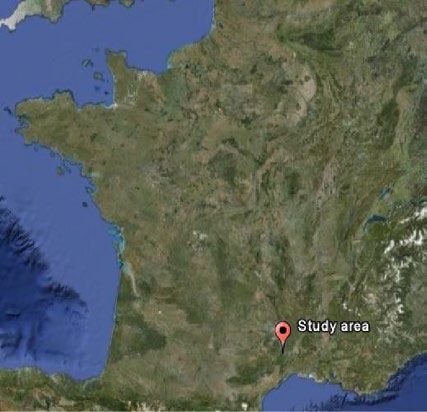
www.nature.com/scientificreports/
Figure 1. Genetic variation among the captured Phlebotomus ariasi individuals. Scatter plot of individuals
based on the first two axes (created from the optimum 13 principal components) of the DAPC. The inset shows
the amount of variation represented by the discriminant analysis eigenvalues. Points and ellipses are colored
according to the groups defined by the DAPC. Misassigned individuals (outliers) are indicated.
two microsatellite loci and other genetic markers were used to understand Ph. ariasi expansion in Europe during
the Pleistocene glacial c ycles23.
However, no population genetics study tackled the influence of geographic (spatial organization) together
with environmental (altitude and hillside) factors in the distribution of sand flies. Therefore, the aims of this
work were to study the structure of Ph. ariasi populations at a local scale, and the impact of environmental fac-
tors (geographical distance, altitude, and hillside) on their spatial organization. For this purpose, sampling was
performed in a well-documented area (Roquedur, Hérault, France), in which sand fly populations were already
orphometrically25 described, and where human and canine leishmaniasis caused by L. infan-
ecologically24 and m
tum are endemic5,26. The analysis was carried out using 11 previously described microsatellite loci for Ph. ariasi27.
Results
Genotyping. In total, 1,253 sand flies were genotyped using the 11 loci described in the Supplementary
Table S1. Sand fly DNA samples in which more than six loci could not be amplified were removed from the
analyses (n = 54 individuals, Group “/” in Supplementary Table S1).
Bayesian clustering. Discriminant analysis of principal components (DAPC) identified 40 clusters with
a mean assignment probability PAss = 0.8568. Twenty individuals were grouped in one strongly differentiated
cluster (cluster 21 with PAss = 1) (Fig. 1). Moreover, two outliers (one from cluster 2 and one from cluster 28) were
close to cluster 21. Bayesian Analysis of Population Structure (BAPS) found 28 clusters (probabilities for number
of clusters = 0.93641). A cluster of 22 individuals (BAPS cluster 28) included the 20 individuals from DAPC clus-
ter 21 and the two outliers highlighted by DAPC. The optimal number of clusters found by STRUCTURE HAR-
VESTER (used to visualize the results of STRUCTURE analysis) was two with ΔK = 16.03 (the second biggest ΔK
was 2.55). Surprisingly, the clusters found by STRUCTURE did not match the DAPC or BAPS results. These two
clusters grouped individuals from several stations with no obvious relation with any ecological or geographical
parameter, and with a very small average assignment probability of individuals to their cluster (PAss = 0.53683).
The partition found by STRUCTURE and STRUCTURE harvester with K = 2 is probably meaningless.
Cytb fragment sequencing of seven individuals from cluster 21 (# 12, 17, 18, 19, 856, 872, and 874) and one
of the two outliers (# 23, cluster 2) showed 99–100% similarity with Ph. ariasi (GenBank accession number:
KP685539.1, and sequences in Supplementary File 1). Therefore, the taxonomic status of the 22 outliers could not
be elucidated. These 22 individuals (Group A in Supplementary Table S1) were all males captured in three stations
(ST02, ST11 and ST12). Neither particular environmental condition nor specific morphological character was
Scientific Reports | (2020) 10:14443 | https://doi.org/10.1038/s41598-020-71319-w 2
Vol:.(1234567890)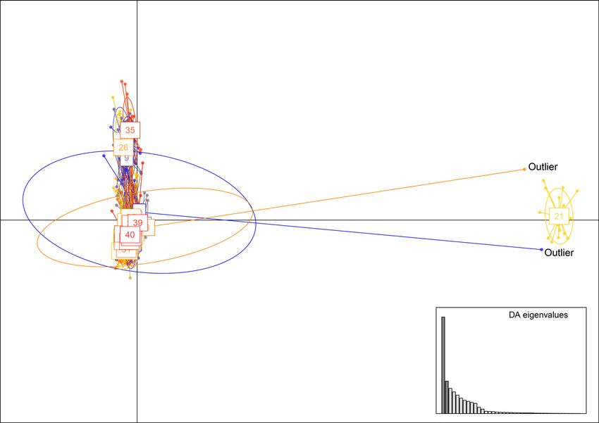
www.nature.com/scientificreports/
0.050
ST02-B
Figure 2. Dendrogram (NJTree) of the genetic relationship between subsamples defined as combinations of
group A or B and sampling station (ST) based on Cavalli-Sforza and Edwards chord distance calculated with six
loci (Aria2, Aria3, Aria4, Aria5, Aria13, and Aria14). Outlier individuals (Group A) are indicated in red. The
same tree was obtained also using 10 loci (excluding Aria1).
recorded for these individuals compared with the other sand fly specimens. The 22 outliers were homozygous for
allele 204 at the Aria1 locus. This allele was not found in the other 1,177 individuals (Group B in Supplementary
Table S1). The dendrogram (NJTree) seems to exclude two subsamples A from all other subsamples, while a third
one appeared fully included within group B (Fig. 2). This structuring appears to be robust since the same tree
was obtained with 6 (Aria2, Aria3, Aria4, Aria5, Aria13, and Aria14, loci selected after Linkage Disequilibrium
(LD) and F-statistics analyses, see below) or 10 loci (excluding Aria1).
Except when specified otherwise, the 22 individuals of Group A were removed from the analyses to prevent
Wahlund effects.
Locus selection for the analyses of Group B sand flies. The Aria1 locus was almost monomorphic
(HS = 0.06) and was removed from the data. Using regression approach we detected a marginally not significant
Short Allele Dominance (SAD) for the Aria14 locus (p value = 0.0507). As SAD results from a preferential ampli-
fication of the shortest allele in heterozygous i ndividuals28, the Aria14 microsatellite profile of each homozygous
individual was checked again following recommendation suggested in De Meeûs et al.29, corrected, and then
analyzed using GENEMAPPER 4.0. After correction, SAD could not be detected on this locus any longer (p
value = 0.0731).
The Micro-Checker analysis suggested stutter artifacts at five loci (Aria2, Aria3, Aria10, Aria14, and
Aria15). The unilateral exact binomial test indicated that the proportion of significant stuttering was not sig-
nificantly higher than the expected proportion under the null hypothesis for Aria2 (p value = 0.2078), Aria3
(p value = 0.2078) and Aria14 (p value = 0.5819). Nevertheless, it was marginally not significant for Aria10 (p
value = 0.0503) and highly significant for Aria15 (p value = 9.728e−06). Therefore, alleles close in size were pooled,
avoiding pooling together only rare alleles (i.e., presence of at least one frequent allele in the pool) for these two
loci as recommended29. As the Aria10 locus became monomorphic after pooling, this locus was removed from
the analysis. For Aria15, alleles 117, 119 and 121 were pooled with allele 123; allele 127 was pooled with allele
125; and allele 131 was pooled with allele 129. However, after correction, the Micro-Checker analysis and the
unilateral exact binomial test (p value = 9.728e−06) highlighted that stuttering still affected this locus. Therefore,
Aria 15 was also removed from the analysis.
On the remaining 9 loci, the linkage disequilibrium (LD) analysis indicated that 7 locus pairs (out of 11)
displayed a significant LD (19.4%). Three of these locus pairs (Aria11 and Aria 12, Aria 11 and Aria 13, Aria
12 and Aria14) remained significant after Benjamini and Yekutieli adjustment. Aria11 and Aria12 displayed
outlier profiles with strongly negative FIS (Fig. 3), above average FST (Fig. 4), large FIS and FST variance (Figs. 3,
4), and strong LD. These results suggested the non-neutrality of these loci. Therefore, Aria11 and Aria12 were
also removed from the analysis.
To check the result stability, additional DAPC analyses were performed by successively removing the following
loci Aria1, Aria10, Aria11, Aria12, and Aria15. As long as Aria1 was kept, the obtained pattern was the same as
in Fig. 2 (data not shown). With the remaining six loci (Aria2, Aria3, Aria4, Aria5, Aria13, and Aria14), DAPC
and BAPS provided no clear structure. This suggested that the distinction between group A (the 22 outliers) and
group B (the 1,177 remaining individuals) only relied on the Aria1 locus (Supplementary Table S1).
Scientific Reports | (2020) 10:14443 | https://doi.org/10.1038/s41598-020-71319-w 3
Vol.:(0123456789)www.nature.com/scientificreports/
0.5
0.4
0.3
0.2
FIS 0.1
0
-0.1
-0.2
-0.3
Aria2 Aria3 Aria4 Aria5 Aria10 Aria11 Aria12 Aria13 Aria14 Aria15 Average Average
0.0001 0.0265 0.1282 0.0654 0.0001 0.9999 0.9999 0.0135 0.0001 0.0001 10 loci 6 loci
0.1667 0.2264 0.4566 1 0.1144 0.7514 0.8659 0.1996 0.07311 0.9923 0.0001 0.0001
2 2 0 0 3 NA NA 0 1 7
Locus
p value for FIS not > 0
p value for short allele dominance
Number of subsamples with stuttering
Figure 3. Deviation from the genotypic proportions expected for panmixia as measured by FIS in Phlebotomus
ariasi for each microsatellite locus and averaged across loci. For each locus, the 95% CI values for subsamples
obtained with the jackknife over subsamples is represented with dashes. The 95% CI values for the average,
with 10 and 6 loci, were obtained by 5,000 bootstraps over loci. The results of tests for panmixia, short allele
dominance, and number of subsamples with stuttering for each locus are also indicated.
0.13
0.11
0.09
0.07
FST
0.05
0.03
0.01
-0.01
Aria2 Aria3 Aria4 Aria5 Aria10 Aria11 Aria12 Aria13 Aria14 Aria15 Average
0.0544 0.0029 0.8994 0.2698 0.3141 0.0001 0.0001 0.8688 0.0048 0.6834 0.0001
Locus
p value (bilateral)
Figure 4. Effect of subdivision (FST value) in Phlebotomus ariasi for each microsatellite locus and averaged
across loci. For each locus, the 95% CI value calculated with the jackknife over subsamples is represented with
dashes. The 95% CI of average was obtained by 5,000 bootstraps over loci.
Linkage disequilibrium and F‑statistics with the six remaining loci. With the remaining six loci
(Aria2, Aria3, Aria4, Aria5, Aria13, and Aria14), the proportion of significant LD tests was 13.3% (two locus
pairs), but none of these tests remained significant after Benjamini and Yekutieli adjustment. There was still a
rather small but significant heterozygote deficit in subsamples (average FIS = 0.059, p value = 0.0001). Variation
across loci appeared pronounced (Fig. 3), but the relationship between FIS and FST was not significant (Spear-
man’s ρ = 0.2319, p value = 0.3292). There was no relationship between the number of missing data at each locus
and the FIS values (ρ = − 0.029, p value = 0.5403). The jackknife method showed that the loci standard error of FIS
Scientific Reports | (2020) 10:14443 | https://doi.org/10.1038/s41598-020-71319-w 4
Vol:.(1234567890)www.nature.com/scientificreports/
Variables Sum2 Pseudo R2 p value
Altitude 0.110675 0.5175 0.0006
Hillside 0.023237 0.1525 0.0002
Longitude 0.011227 0.0769 0.1663
Latitude 0.001147 0.0361 0.1430
All 0.7830
Table 1. Minimum model obtained for the regression of PCA axis 2 coordinates of Phlebotomus ariasi
sampling sites. The sum of squares (Sum2), the proportion of deviance explained by the model and the
proportion of deviance explained for each explanatory variable (Pseudo R2) are given. The p values were
obtained after F tests.
was 0.055 and was 27 times bigger than that for FST (0.002). The Micro-Checker analysis suggested the presence
of null alleles at four loci (Aria2, Aria3, Aria4, and Aria14). According to the criteria described in De Meeûs30
(see “Methods” section), null alleles only explained partly (if any) the observed heterozygote deficit.
To check the result stability again, the FIS computed for the dataset that included also Group A (complete
dataset) was compared with the one obtained without it (Group B) (Supplementary Table S1). The FIS was bigger
in the complete dataset than in Group B alone (FIS = 0.079 and FIS = 0.057, respectively), and the difference was
significant (p value = 0.0486 unilateral Wilcoxon signed rank test). This translated into a Wahlund effect when
Group A individuals were included in the data. These individuals were thus kept excluded.
Regression approach. A Principal Component Analysis (PCA) was undertaken with PCAGen (developed
by J. Goudet, freely available at https://www2.unil.ch/popgen/softwares/pcagen.htm). The first two axes were
significant using the broken stick criterion but not by permutation testing (p value = 0.2187 for axis 1 and p
value = 0.1045 for axis 2) (see “Methods” section). Axis 1 and axis 2 represented 31% and 23% of the total inertia,
respectively. We undertook two generalized linear model (glm) with the coordinates of subsamples at these axes
(see “Methods” section). For the first axis, the minimum model, after a stepwise procedure, was: axis1 ~ hill-
side + latitude + longitude + latitude:hillside. For this axis, none of the included variables played a significant role
(p value > 0.05 for all tests). For axis 2, the minimum model was: axis2 ~ hillside + altitude + latitude + longitude.
Altitude and hillside played a significant role (p values < 0.001) and represented 51% and 15% of the total devi-
ance, respectively (Table 1).
Isolation by altitude distance. As showed above, latitude and longitude had a weak effect on the genetic
structure. Geographic parameters were thus removed from the model and isolation by altitudinal distance was
tested using the Mantel test for each hillside separately (South–East and North–West, two tests).
When individuals were grouped by altitude levels (see Table 2 and “Methods” section), isolation by altitude
distance was significant for the Northern (p value = 0.00605) and marginally non-significant for the Southern
hillside (p value = 0.07345). When combined with the generalized binomial p rocedure31, computed with the
MultiTest V132, isolation by altitude appeared highly significant (p value = 0.0054).
Effective population sizes and migration. The average effective population size (Ne) was 69 individuals
(range: 39 to 98) across subsamples and methods (see “Methods” section). Ne was not correlated with altitude
(Spearman’s ρ = 0.2216, p value = 0.7864). There was no effect of hillside (Kruskal–Wallis p value = 0.6242). Nei’s
unbiased estimator of genetic diversities33 was HS = 0.52 and HT = 0.524 for the subsamples and total sample,
respectively, with Meirmans and Hedrick’s GST’’ = 0.01734, and then Nem = (1 − GST’’)/4 GST’’ = 14 (immigrants
per generation in each subpopulation assuming an island model of migration). The correlation between Nei’s
GST and HS was strongly negative (rho = − 0.94, p value = 0.0083). Therefore, according to Wang’s criterion35, it is
more accurate using FST. FST with the ENA correction for null alleles and 95% confidence intervals (95% CI) after
5,000 bootstraps over loci were computed with FreeNA36. This provided FST = 0.014 (95% CI = [0.006, 0.023]),
with a corresponding Nem = 18 (95% CI [10, 40]).
Discussion
Locus selection. In this study, using 11 microsatellite markers, we investigated the genetic structure of Ph.
ariasi populations in 1,253 individuals collected in 17 stations in the South of France (Supplementary Table S1).
Different analyses (Micro-Checker, LD, FIS and FST variance) allowed identifying loci with technical problems
and/or loci that may not be neutral concerning natural selection. Consequently, we removed five of the eleven
loci for various reasons including the presence of incurable stutter artifacts (Aria10 and Aria15), absence of
polymorphism (Aria1), or non-neutral evolution (Aria11 and Aria12). One locus with SAD could be corrected.
Presence of outlier individuals. The Bayesian analyses (DAPC and BAPS) for all remaining loci (Aria2,
Aria3, Aria4, Aria5, Aria13, and Aria14) confirmed the 22 outliers (Group A). These outliers were morphologi-
cally similar to Ph. ariasi and displayed 99–100% cytb sequence similarities. A previous study, based on chroma-
tographic analysis of cuticular components, provided evidence that there are two distinct Ph. ariasi populations
in our study area: one predominantly sylvatic, and the second one d omestic19. However, in our study, there was
no geographical distribution difference between individuals from Group A and Group B.
Scientific Reports | (2020) 10:14443 | https://doi.org/10.1038/s41598-020-71319-w 5
Vol.:(0123456789)www.nature.com/scientificreports/
Station UTM E UTM N HO Alt HG Biotope characteristics N
ST01 31T554956 31T4868394 SE 228 A1 Hamlet 2
ST02 31T554800 31T4868471 SE 244 A1 Hamlet 42
ST03 31T554210 31T4869275 SE 321 A2 Hamlet/Hutch 56
ST04 31T554302 31T4869424 SE 322 A2 Hamlet outskirts 148
ST05 31T554343 31T4869526 SE 341 A2 Kennel 20
ST06 31T554175 31T4869464 SE 354 A2 Hamlet 121
ST07 31T552692 31T4869246 NW 603 A3 Hamlet 9
ST08 31T552715 31T4869102 NW 603 A3 Hamlet 70
ST09 31T552614 31T4868909 NW 573 A3 Countryside 121
ST10 31T552143 31T4869102 NW 539 A3 Countryside 126
ST11 31T551130 31T4868999 NW 417 A4 Countryside 166
ST12 31T550944 31T4869286 NW 397 A4 Countryside 65
ST13 31T550925 31T4869586 NW 362 A4 Countryside 126
ST14 31T550354 31T4869799 NW 343 A5 Countryside 9
ST15 31T549998 31T4870371 NW 282 A5 Hamlet outskirts 116
ST16 31T549453 31T4870290 NW 255 A5 Hamlet 21
ST17 31T549306 31T4870270 NW 245 A5 Hamlet/Sheep barn 35
Table 2. Sampling stations (ST) in the study area. Station names, Universal Transverse Mercator (UTM)
coordinates, hillside orientation (HO) (SE: South–East; NW: North–West), altitude (Alt, in m), hillside group
(HG), biotope characteristics, and number of genotyped sand flies (N) are indicated. A1 (Southern hillside,
100–300 m), A2 (Southern hillside, 300–500 m), A3 (Northern hillside, > 500 m), A4 (Northern hillside,
300–500 m), A5 (Northern hillside, 100-300 m).
This finding could reflect the existence of cryptic species, as already suspected or reported for other sand fly
species (e.g., Lutzomyia longipalpis37,38, Lutzomyia umbratilis39, and Sergentomyia bailyi40). However, the distinc-
tion between Group A and Group B mainly depends on a single genetic marker (Aria1), which is fixed for dif-
ferent alleles in each group, while the other markers display a rather weak, though significant, signal. This result
is supported by the dendrogram as the same tree was obtained with 6 or 10 loci (excluding Aria1). Additional
molecular and biological studies will be necessary to test the cryptic species hypothesis (vector competence,
interbreeding, hosts and niche preferences, behavior, etc.). As the taxonomic status of Group A individuals could
not be elucidated, they were removed from the analyses.
Genetic structuring in ecotypes. We observed an important and significant heterozygote deficit, instead
of the heterozygote excess expected for dioecious populations with random m ating41. We found no evidence of
42
Wahlund effect with the LD-based method described by Manangwa et al. . Consequently, the heterozygote defi-
cit could (non-exclusively) be explained by (1) null alleles; (2) allelic dropout; or (3) positive assortative mating.
In the last case, this would require a mutual attraction of sexual partners based on a sufficient proportion of the
genome to allow the hitchhiking of microsatellite markers, which are theoretically non-coding DNA sequences.
The glm approach showed a strong influence of altitude and hillside, and a weak (if any) influence of geo-
graphic distances on the genetic data. The proportion of deviance (67%) explained by altitude and hillside sug-
gested the existence of ecotypes in this Ph. ariasi population.
The very strong migration rate estimated in our study (more than 25% of the effective subpopulation size)
is hard to reconcile with the emergence of genetically distinct ecotypes. Different scenarios can explain ecotype
structuring despite the strong migration rate: (1) the death of most immigrants before they can reproduce
(unlikely scenario), and (2) significant assortative mating that can also explain the heterozygote deficit observed
in our data (see above). The rate of codominant assortative mating based on genes homogeneously distributed
in the genome can be approximated with the same equation as for selfing, as described in Hartl et al.43 (page
272), with the equation a ≈ 2FIS/(1 + FIS). With a FIS = 0.057, the assortative mating in our population would be
≈ 0.11 (≈ 11% of zygotes produced).
It is worth noting that previous research on the same species in the same study area highlighted differences
in wing phenotypes according to altitude and h illside25. It has been demonstrated that wing configuration is
associated with wing beating frequency and mate recognition44,45. These features would lead to a preferential
choice of partners that could explain assortative mating and ecotype structuring. More studies are necessary to
investigate the link between phenotypic (wing configuration) and genetic (microsatellite) diversity.
Ecological and epidemiological consequences of this genetic structuration. This structuring
has undoubtedly implications on the ecology and evolution of sand flies. This structure might favor the global
stability of their populations. Indeed, local environmental changes would have no or low effect on the overall
population because the ecotypes would be affected independently. The high levels of migration rates associated
with the well-known low capacity of flying of sand flies would help to colonize and recolonize at small-scale
Scientific Reports | (2020) 10:14443 | https://doi.org/10.1038/s41598-020-71319-w 6
Vol:.(1234567890)www.nature.com/scientificreports/
Data SIO, NOAA, U.S. Navy, NGA, GEBCO
A Image Landsat / Copernicus B
© 2020 Google
© 2020 GeoBasis-DE/BKG
Le Vigan
C Lodève
St Julien
de la Nef
A1 A2 A3 A4 A5
Sta ons
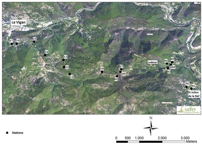
Figure 5. Localization (A), map (B) and profile (C) of the study area. Red dots and numbers indicate the
sampling stations. A1 (Northern hillside, 100–300 m), A2 (Northern hillside, 300–500 m), A3 (Northern
hillside, > 500 m), A4 (Southern hillside, 300–500 m), and A5 (Southern hillside, 300–100 m). The map came
from three sources ([A] Google Earth, [B] SAFER and [C] adapted from Rioux et al.3 "Creative Commons
license") that were combined under Adobe Illusrator.
e nvironments46. It also could explain the global but slow (compared with that of invasive mosquitoes, such as
Aedes albopictus) geographical expansion of sand flies observed in France17.
This particular population structure can also influence Leishmania transmission. Previous studies suggested
the existence of different imbricated Leishmania transmission cycles at very small scales47,48. However, due to the
low flying capacities of sand fl ies46,49, migrants are expected to disperse mainly over short distances. Therefore,
the spread and increase of L. infantum cases in France might be mainly due to the movement of infected hosts.
This study demonstrates for the first time that Ph. ariasi presents a genetic structure in ecotypes. These data
highlight the necessity to consider sand fly populations at small and specific scales to determine their ecology and
its impact on Leishmania transmission. This structure may explain the long-term stability of sand fly populations.
Not many papers compare available clustering algorithms to date and it is thus hard to really understand when
and why such algorithms will converge or diverge in the best partition they offer. For some attempt comparisons
see: Latch et al.50, Kaeuffer et al.51, Frantz et al.52, Blair et al.53, Bohling et al.54, Manangwa et al.42.
This type of study needs to be extended to other sand fly species. Indeed, the large diversities of sand fly popu-
lations worldwide may correlate with different ecological vector capacities and sensitivity to control measures.
Methods
Study area. The field study was performed in the South of France, on the “massif de l’Oiselette” hill situated
between the “Hérault” (Ganges, Hérault) and “Arre” (Le Vigan, Gard) valleys. Sand flies were sampled along a
14 km transect from the “Saint Julien de la Nef ” to “Le Vigan” villages, including “Roquedur-le-haut” (at 601 m
above sea level) (Fig. 5; Table 2). This region has a Mediterranean sub-humid c limate55, and is characterized by
the presence of plant species typical of scrubland habitats5.
The study area was divided in two hillsides with a South–East and North–West orientation, like in previous
works performed in this a rea3,24,25. Stations were selected based on the paper of Rioux et al.3, first to allow the
comparison with the data obtained 30 years ago in terms of species distribution, density and abundance24, sec-
ond because these stations were distributed along the 14 km transect and represented the altitude and hillside
diversity necessary for our population genetics study. Station 7 and Station 8 were not present in Rioux et al.3.
These two stations are transitional between the two hillsides, and were thus added in the present study to obtain
information on the consequences of transitional ecosystems. The stations were grouped according to altitude
and hillside (see Fig. 5; Table 2). This area is characterized by the presence of various domestic animals, such
as chicken, sheep, ducks, geese, horses, rabbits, cats, dogs, and also many different wild animals (wild boars,
foxes, rodents, lizards, birds, etc.). These animals represent potential sand fly hosts. Moreover, cases of canine
leishmaniasis were observed during the collection period (J.P. personal observation).
Scientific Reports | (2020) 10:14443 | https://doi.org/10.1038/s41598-020-71319-w 7
Vol.:(0123456789)www.nature.com/scientificreports/
Sand fly collection and identification. Sand flies were collected monthly using 3,589 sticky traps
(20 × 20 cm white paper covered with castor oil, as described by Alten et al.56 and Ayhan et al.57) between May
and September 2011. Seventeen localities (sampling stations) were sampled (Fig. 5; Table 2) with a mean of 189
sticky traps per station, in various biotopes, inside and around human dwellings and animal sheds, close to the
vegetation, and in wall crevices. Each trap was collected after 2 days.
In total, 1,253 sand flies were captured and transferred individually into 1.5 mL Eppendorf tubes with 96%
ethanol and labeled. Prior to mounting, the sand fly head, genitalia and wings were removed. Heads and geni-
talia were cleared in Marc-André solution (chloral hydrate/acetic acid) and mounted in chloral g um46. Each
individual specimen was identified on the basis of the morphology of the pharynges and/or male genitalia or
female spermathecae, using the keys of A bonnenc46, Lewis6 and Killick-Kendrick et al.58.
DNA extraction. Sand fly DNA was extracted using the Chelex method59 described in Prudhomme et al.27.
Extraction was performed at the UMR “Unité des Virus Emergents” (UVE, IHU Méditerranée Infection, Mar-
seille, France). Each entire sand fly was ground using a Mixer Mill MM300 (QIAGEN, Venlo, Netherlands) with
one 3-mm tungsten bead in 200 μL Eagle’s Minimal Essential Medium at a frequency of 30 cycles s −1 for 3 min.
A volume of 140 μL of each sample was then used for DNA purification by adding the Chelex resin s uspension59
or by using the Eppendorf epMotion 5075 working station and the Macherey–Nagel NucleoSpin 96 Virus kit.
DNA amplification and genotyping. Based on the microsatellite position in the sequence and the
repeated pattern structure, 11 of the most polymorphic loci were selected among the previously described 16
microsatellite markers for Ph. ariasi27. Each 25 μL reaction mix included 1 pmol of forward (labeled with the
fluorochrome FAM, ATT0565 or HEX) and reverse primers, 5 ng of sand fly DNA sample, 6 pmol of dNTP mix,
2.5 μL of 10X buffer, and 0.25 μL of Taq polymerase (ROCHE DIAGNOSTICS, 5 UI/μL). DNA was amplified in a
thermal cycler using the following conditions: initial denaturation step at 95 °C for 10 min, followed by 40 cycles
at 95 °C for 30 s, the specific annealing temperature of each locus27 for 30 s, 72 °C for 1 min, and a final exten-
sion step at 72 °C for 10 min. For genotyping, 1 μL of PCR product was added into a standard loading mix (0.5
μL of the internal GeneScan 500LIZ dye size standard and 12.5 μL of Hi-Di formamide) (both from APPLIED
BIOSYSTEMS) and sequenced on an ABI Prism 3130 Genetic Analyzer (APPLIED BIOSYSTEMS) automated
sequencer. Profiles were read and analyzed using GENEMAPPER 4.0 [APPLIED BIOSYSTEMS, Foster City
(CA)].
DNA from a subset of Ph. ariasi samples was used to check the species identification (see “Results” section)
by amplifying a cytb gene fragment using the primers N1N-PDR [5′-CA(T/C) ATT CAA CC(A/T) GAA TGA
TA-3′] and C3B-PDR [5′-GGT A(C/T)(A/T) TTG CCT CGA (T/A)TT CG(T/A) TAT GA-3′], according to a
previously published p rotocol60,61 and the following conditions: initial denaturation at 94 °C of 3 min; 5 cycles
of denaturation (94 °C for 30 s), annealing (40 °C for 60 s), and extension (68 °C for 60 s), followed by 40 cycles
of denaturation (94 °C for 60 s), annealing (44 °C for 60 s) and extension (68 °C for 60 s), and a final extension
(68 °C for 10 min). Direct sequencing in both directions was performed by Eurofins Genomics.
Data analysis. Microsatellite raw data were formatted for C
REATE62 that allowed their transformation into
the formats needed for the different analyses. Samples with more than 50% of missing data were removed from
the analyses.
Bayesian clustering. Several Bayesian clustering analyses were carried out. To validate the sand fly species iden-
tification, the first analysis was based on the 11 selected loci and included all sand fly samples. Then, to study the
organization of Ph. ariasi populations, data were analyzed at different scales: hillside, altitude, and station. This
analysis was performed with the loci selected after Linkage Disequilibrium (LD) and F-statistics analyses (see
“Results” section).
As the clustering method accuracy can vary depending on the statistical properties of specific software pro-
grams and datasets29,42,63, three different Bayesian clustering methods were used. First, a discriminant analysis
of principal components (DAPC)64 was performed using the adegenet65 package for R66. This was followed by a
Bayesian Analysis of Population Structure (BAPS; admixture model67,68, maximum number of clusters: 35, rep-
etition: 50; that is freely available at https://www.helsinki.fi/bsg/software/BAPS/), and a STRUCTURE (version
2.3.4) analysis69 (burning period: 10,000, number of clusters from 1 to 35, with the admixture model). STRU
CTURE HARVESTER vA.270 was used to visualize the STRUCTURE analysis results, examine the ad hoc ΔK
statistic, and determine the optimal number of clusters.
Finally, a dendrogram (NJTree) was built with MEGA 771 from a Cavalli-Sforza and Edward’s chord distance
(DCSE)72 matrix as recommended73, between subsamples defined as combinations of the group obtained by
Bayesian clustering and sampling stations. Because null alleles were suspected to occur, DCSE was computed
with the INA correction with F reeNA36, after recoding missing data into null homozygotes following authors’
recommendation.
Linkage disequilibrium and F‑statistics. LD between each locus pair was tested with the G-based permutation
test with 10,000 randomizations. This test was performed with F STAT 2.9.374
STAT 2.9.4, an updated version of F
available at https://www.t-de-meeus.fr/ProgMeeusGB.html. This procedure is the most powerful for testing LD
across different s ubsamples32. There are as many p values as locus pairs. Then, the False Discovery Rate (FDR)
correction for multiple non-independent tests described by Benjamini et al.75 was applied with R 3.5.166.
Scientific Reports | (2020) 10:14443 | https://doi.org/10.1038/s41598-020-71319-w 8
Vol:.(1234567890)www.nature.com/scientificreports/
Wright’s F statistics76 were estimated with the Weir and Cockerham’s unbiased e stimators77. Significant depar-
ture from 0, for F statistics, was tested by randomizing alleles between individuals within subsamples (deviation
from the local random mating test) or individuals between subsamples within the total sample (population
subdivision test). The p value corresponded to the number of times a statistic measured in randomized samples
was as big as (or bigger than) the observed one (unilateral tests). For local panmixia, the statistic used was f (Weir
and Cockerham’s FIS estimator). To test for subdivision, the G-based test78 was used. According to De Meeûs
et al.32, the G-based test is the most powerful procedure when combining tests across loci.
The 95% confidence intervals (CI) of F-statistics were computed using the jackknife over populations method
for each locus or 5,000 bootstraps over loci for the averages, as described in De Meeûs et al.79. Parameter esti-
mates, testing, jackknife and bootstrap computations were done with FSTAT2.9.4.
The determination procedure described by De Meeûs30 and Manangwa et al.42 was used to discriminate
demographic from technical causes of significant homozygote excess and LD. In the case of null alleles, FIS and
FST artificially increase and a positive correlation is expected between the statistics, FIS standard error is at least
twice that of FST, and a positive correlation is also expected between FIS and the number of missing data (putative
null homozygotes). Correlations were tested with the unilateral Spearman’s rank correlation test in R 3.5.166. The
frequency of null alleles was assessed with Micro-Checker v2.2.380 using Brookfield’s second m ethod81.
The presence of stutter artifacts at each locus in each subsample was evaluated with Micro-Checker v2.2.380. A
unilateral exact binomial test was used with R 3.5.166 to determine whether the observed proportion of significant
stutter artifacts was greater than the expected 5% under the null hypothesis.
Short Allele Dominance (SAD) was assessed with the method described by Manangwa et al.42. The correlation
between allele size and FIT was tested with the unilateral Spearman’s rank correlation test in R 3.5.166. In the case
of SAD, a negative correlation is expected between allele size and FIT42.
In the case of significant stutter artifacts or SAD, the incriminated loci were corrected using the method
described by De Meeûs et al.29. Stuttering was addressed by pooling alleles close in size. To avoid a spurious
increase of heterozygosity, each pooled group contained at least one frequent allele (e.g., with p value ≥ 0.05).
SAD was addressed by going back to the chromatograms of homozygous individuals and trying to find a larger
size micro-peak that could have been missed in the first reading.
In some instances, FIS values were compared between subsample groups using the Wilcoxon signed rank test
for paired data (the locus was the pairing unit).
Role of environmental factors on sand fly structuring. A principal component analysis (PCA) was done with
PCAGen 1.2.1 (developed by J. Goudet, freely available at https://www2.unil.ch/popgen/softwares/pcagen.htm).
The significance of the first axes was tested using the broken stick c riterion82 and 10,000 permutations of indi-
viduals across subsamples. The metric of each axis divided by the total genetic diversity corresponded to Weir
& Cockerham’s Theta (FST estimator) (Goudet’s personal communication). The coordinates of subsamples for
each significant axis were used as the response variable of generalized linear models (glm). General models were
as follows: axis i ~ latitude + longitude + altitude + hillside + latitude: hillside + longitude:hillside + altitude:hillside
(where i corresponded to the significant axes; latitude and longitude are the latitudinal and longitudinal GPS
coordinates in decimal degrees; altitude is the altitude in meters; hillside: south–east or north–west; and "X:Y"
represents the interaction between the explanatory variables X and Y). All glm’s were done using R version
3.5.166, with the package rcmdr (R-commander)83,84. Model selection was performed using a forward stepwise
model selection procedure and the Akaike Information Criterion85.
The influence of different factors (including interactions) was tested by examining the differences between
models (complete, additive, and with one variable) with analyses of variances. As the entry order of explanatory
variables matters in R analyses, the mean partial R2 of each variable was calculated across all possible models.
Isolation by distance. Geographic distances were computed with Genepop version 4.7.086 using the Euclidian
distance computed with the Universal Transverse Mercator (UTM) coordinates (Table 2). Genetic distances
were estimated with the Cavalli-Sforza and Edwards chord d istance72 DCSE, the most powerful method to detect
isolation by distance with microsatellite markers in most situations87. Due to the presence of missing data, data
were converted into the FreeNA format to compute DCSE between each station pair with the ENA c orrection36
that provides a very good correction for the isolation by distance regression slope in the case of null alleles87.
As these station pair ended into a non‐squared matrix that could not be handled by Genepop, the relationships
between genetic and geographic distances were tested with a Mantel test ( 104 permutations)88 in FSTAT 2.9.4. As
the Mantel test in FSTATis bilateral by default, the p value was halved in the case of positive slope, or computed as:
“1-(1-bilateral p values)/2” in the case of negative slope, to obtain unilateral p values for a positive slope.
The relationships between genetic and altitudinal distances were also tested in the conditions described above.
To avoid any interaction, the analyses for the South and North hillsides were done separately. The two p values
obtained were then combined with the generalized binomial t est31, with M ultiTest32, taking into account all tests
as recommended when the number of combined tests k < 489.
Effective population sizes and migration. Four different methods were used to estimate the effective popula-
tion sizes (Ne). The results obtained with these methods were averaged and weighted by the number of times a
usable value (after removal of “infinity” results) was obtained. To obtain a range of possible Ne values, the same
approach was performed for the minimum and maximum values obtained with each method.
First, NeEstimator v290 was used with the LD method91,92 that applies a correction for missing data93 and the
molecular co-ancestry method94. The LD method uses several threshold allele frequencies (0.05, 0.02, 0.01, and
all alleles) to compute Ne. The average across the different values obtained with these frequencies was computed.
Scientific Reports | (2020) 10:14443 | https://doi.org/10.1038/s41598-020-71319-w 9
Vol.:(0123456789)www.nature.com/scientificreports/
The intra- and inter-loci correlation method was also used to compute Ne95 using Estim v2.296 (available at:
https://www.t-demeeus.fr/ProgMeeusGB.html).
Finally, the heterozygote-excess method (expected in dioecious populations) described by B alloux41 was used
for each locus that displayed heterozygote excess, as follows: Ne = [− 1/(2 FIS)] −FIS/(1 + FIS).
To determine the number of immigrants, the standardized differentiation index described by Meirmans and
Hedrick was computed to correct for polymorphism excess: GST" = n × (HT − HS)/[(n × HT − HS) × (1 − HS)]34,
where HT and HS are Nei’s unbiased estimates of genetic diversity in the total sample or within subsamples,
respectively33, and n is the number of subsamples. Genetic diversities were estimated with F STAT 2.9.4. Assum-
ing an island model, this value was then used to obtain an approximation for the number of immigrants within
subpopulations as Nem = (1 − GST")/(4 × GST"). However, according to Wang’s criterion35 if Nei’s GST33 is negatively
correlated with HS, it is wiser to use FST for this computation.
Data availability
All resources used in this article are provided in the Supporting Information and all the analyses are detailed
allowing the assessment or verification of the manuscript’s findings.
Received: 3 April 2020; Accepted: 15 July 2020
References
1. Dolmatova, A. V. & Demina, N. A. Les phlébotomes (Phlebotominae) et les maladies qu’ils transmettent. ORSTOM 20, 1–169
(1966).
2. Bichaud, L. et al. Epidemiologic relationship between toscana virus infection and Leishmania infantum due to common exposure
to Phlebotomus perniciosus sandfly vector. PLoS Negl. Trop. Dis. 5(9), e1328 (2011).
3. Rioux, J.-A., Killick-Kendrick, R., Perieres, J., Turner, D. & Lanotte, G. Ecologie des Leishmanioses dans le sud de la France. 13.
Les sites de “flanc de coteau”, biotopes de transmission privilégiés de la Leishmaniose viscérale en Cévennes. Ann . Parasitol. Hum.
Comp. 55(4), 445–453 (1980).
4. Rioux, J.-A. et al. Ecology of leishmaniasis in the South of France. 22. Reliability and representativeness of 12 Phlebotomus ariasi,
P. perniciosus and Sergentomyia minuta (Diptera: Psychodidae) sampling stations in Vallespir (eastern French Pyrenees region).
Parasite 20, 34 (2013).
5. Rioux, J.-A. et al. Epidémiologie des leishmanioses dans le Sud de la France. Monogr. l’Inst. Natl. Santé Rech. Méd. 20, 1–228 (1969).
6. Lewis, D. J. A taxonomic review of the genus Phlebotomus (Diptera: Psychodidae). Bull. Br. Museum 45(2), 121–209 (1982).
7. Rossi, E. et al. Mapping the main Leishmania phlebotomine vector in the endemic focus of the Mt. Vesuvius in southern Italy.
Geospat. Health 1(2), 191–198 (2007).
8. Ballart, C., Barón, S., Alcover, M. M., Portus, M. & Gallego, M. Distribution of phlebotomine sand flies (Diptera: Psychodidae) in
Andorra: First finding of P. perniciosus and wide distribution of P. ariasi. Acta Trop. 122(1), 155–159 (2012).
9. Ballart, C. et al. Importance of individual analysis of environmental and climatic factors affecting the density of Leishmania vectors
living in the same geographical area: The example of Phlebotomus ariasi and P. perniciosus in northeast Spain. Geospat. Health 8(2),
389–403 (2014).
10. Boussaa, S., Neffa, M., Pesson, B. & Boumezzough, A. Phlebotomine sandflies (Diptera: Psychodidae) of southern Morocco: Results
of entomological surveys along the Marrakech-Ouarzazat and Marrakech-Azilal roads. Ann. Trop. Med. Parasitol. 104(2), 163–170
(2010).
11. Franco, F. et al. Genetic structure of Phlebotomus (Larroussius) ariasi populations, the vector of Leishmania infantum in the western
Mediterranean: Epidemiological implications. Int. J. Parasitol. 40(11), 1335–1346 (2010).
12. Ready, P. Leishmaniasis emergence in Europe. Euro Surveill. 15(10), 19505 (2010).
13. Branco, S. et al. Entomological and ecological studies in a new potential zoonotic leishmaniasis focus in Torres Novas municipality,
Central Region, Portugal. Acta Trop. 125(3), 339–348 (2013).
14. Barón, S. D. et al. Risk maps for the presence and absence of Phlebotomus perniciosus in an endemic area of leishmaniasis in
southern Spain: Implications for the control of the disease. Parasitology 138(10), 1234–1244 (2011).
15. Boudabous, R. et al. The phlebotomine fauna (Diptera: Psychodidae) of the eastern coast of Tunisia. J. Med. Entomol. 46(1), 1–8
(2009).
16. European Centre for Disease Prevention and Control E. Phlebotomine sand flies maps [internet] 2019 [10/01/19]. https://www.
ecdc.europa.eu/en/disease-vectors/surveillance-and-disease-data/phlebotomine-maps.
17. Dedet, J.-P. Les leishmanioses en France métropolitaine. BEH Hors-Sér. 2010, 9–12 (2020).
18. Depaquit, J., Grandadam, M., Fouque, F., Andry, P.-E. & Peyrefitte, C. Arthropod-borne viruses transmitted by Phlebotomine
sandflies in Europe: A review. Euro Surveill. 15(10), 19507 (2010).
19. Kamhawi, S. et al. Two populations of Phlebotomus ariasi in the Cévennes focus of leishmaniasis in the south of France revealed
by analysis of cuticular hydrocarbons. Med. Vet. Entomol. 1(1), 97–102 (1987).
20. Pesson, B., Wallon, M., Floer, M. & Kristensen, A. Étude isoenzymatique de populations méditerranéennes de phlébotomes du
sous-genre Larroussius. Parassitologia 33, 471–476 (1991).
21. Ballart, C., Pesson, B. & Gallego, M. Isoenzymatic characterization of Phlebotomus ariasi and P. perniciosus of canine leishmaniasis
foci from Eastern Pyrenean regions and comparison with other populations from Europe. Parasite. 25, 3 (2018).
22. Martin-Sanchez, J., Gramiccia, M., Pesson, B. & Morillas-Marquez, F. Genetic polymorphism in sympatric species of the genus
Phlebotomus, with special reference to Phlebotomus perniciosus and Phlebotomus longicuspis (Diptera, Phlebotomidae). Parasite
7(4), 247–254 (2000).
23. Mahamdallie, S. S., Pesson, B. & Ready, P. D. Multiple genetic divergences and population expansions of a Mediterranean sandfly,
Phlebotomus ariasi, in Europe during the Pleistocene glacial cycles. Heredity 106(5), 714–726 (2010).
24. Prudhomme, J. et al. Ecology and spatiotemporal dynamics of sandflies in the Mediterranean Languedoc region (Roquedur area,
Gard, France). Parasit. Vectors 8(1), 1–14 (2015).
25. Prudhomme, J. et al. Ecology and morphological variations in wings of Phlebotomus ariasi (Diptera: Psychodidae) in the region
of Roquedur (Gard, France): A geometric morphometrics approach. Parasit. Vectors 9(1), 578 (2016).
26. Lachaud, L. et al. Surveillance of leishmaniases in France, 1999 to 2012. Euro Surveill. 18(29), 20534 (2013).
27. Prudhomme, J. et al. New microsatellite markers for multi-scale genetic studies on Phlebotomus ariasi Tonnoir, vector of Leishmania
infantum in the Mediterranean area. Acta Trop. 142, 79–85 (2015).
28. Wattier, R., Engel, C. R., Saumitou-Laprade, P. & Valero, M. Short allele dominance as a source of heterozygote deficiency at
microsatellite loci: Experimental evidence at the dinucleotide locus Gv1CT in Gracilaria gracilis (Rhodophyta). Mol. Ecol. 7(11),
1569–1573 (1998).
Scientific Reports | (2020) 10:14443 | https://doi.org/10.1038/s41598-020-71319-w 10
Vol:.(1234567890)www.nature.com/scientificreports/
29. De Meeûs T, Chan CT, Ludwig JM, Tsao JI, Patel J, Bhagatwala J, Beati L. Deceptive combined effects of short allele dominance
and stuttering: An example with Ixodes scapularis, the main vector of Lyme disease in the U.S.A. peerreviewed and recommended
by PCI Evolutionary Biology. 2019.
30. De Meeûs, T. Revisiting, FIS, FST, Wahlund Effects, and Null Alleles. J. Hered. 109(4), 446–456 (2018).
31. Teriokhin, A. T., De Meeûs, T. & Guegan, J. F. On the power of some binomial modifications of the Bonferroni multiple test. J.
Gener. Biol. 68(5), 332–340 (2007).
32. De Meeûs, T., Guégan, J.-F. & Teriokhin, A. T. MultiTest V.1.2., a program to binomially combine independent tests and perfor-
mance comparison with other related methods on proportional data. BMC Bioinform. 10(1), 443 (2009).
33. Nei, M. & Chesser, R. K. Estimation of fixation indices and gene diversities. Ann. Hum. Genet. 47(3), 253–259 (1983).
34. Meirmans, P. G. & Hedrick, P. W. Assessing population structure: FST and related measures. Mol. Ecol. Resour. 11(1), 5–18 (2011).
35. Wang, J. Does GST underestimate genetic differentiation from marker data? Mol. Ecol. 24(14), 3546–3558 (2015).
36. Chapuis, M. P. & Estoup, A. Microsatellite null alleles and estimation of population differentiation. Mol. Biol. Evol. 24(3), 621–631
(2007).
37. Maingon, R. et al. Genetic identification of two sibling species of Lutzomyia longipalpis (Diptera: Psychodidae) that produce distinct
male sex pheromones in Sobral, Ceará State, Brazil. Mol. Ecol. 12(7), 1879–1894 (2003).
38. Bauzer, L. G., Souza, N. A., Maingon, R. D. & Peixoto, A. A. Lutzomyia longipalpis in Brazil: A complex or a single species? A
mini-review. Mem. Inst. Oswaldo Cruz. 102(1), 1–12 (2007).
39. Scarpassa, V. M. & Alencar, R. B. Lutzomyia umbratilis, the main vector of Leishmania guyanensis, represents a novel species
complex? PLoS One 7(5), e37341 (2012).
40. Tharmatha, T., Gajapathy, K., Ramasamy, R. & Surendran, S. N. Morphological and molecular identification of cryptic species in
the Sergentomyia bailyi (Sinton, 1931) complex in Sri Lanka. Bull. Entomol. Res. 107(1), 58–65 (2016).
41. Balloux, F. Heterozygote excess in small populations and the heterozygote-excess effective population size. Evolution 58(9), 1891–
1900 (2004).
42. Manangwa, O. et al. Detecting Wahlund effects together with amplification problems: Cryptic species, null alleles and short allele
dominance in Glossina pallidipes populations from Tanzania. Mol. Ecol. Resour. 19(3), 757–772 (2019).
43. Hartl, D. L. & Clarck, A. G. Principles of Population Genetics 2nd edn. (Sinauer Associates Inc, Sunderland, 1989).
44. Araki, A. S. et al. Multilocus analysis of divergence and introgression in sympatric and allopatric sibling species of the Lutzomyia
longipalpis complex in Brazil. PLoS Negl Trop Dis. 7(10), e2495 (2013).
45. Kyriacou, C. Sex and rhythms in sandflies and mosquitoes: an appreciation of the work of Alexandre Afranio Peixoto (1963–2013).
Infect. Genet. Evol. 28, 662–665 (2014).
46. Abonnenc E. Les phlébotomes de la région éthiopienne (Diptera, Psychodidae): Cahiers de l’ORSTOM, série Entomologie médicale
et Parasitologie; 1972 01/01. 239.
47. Rougeron, V. et al. Reproductive strategies and population structure in Leishmania: Substantial amount of sex in Leishmania
Viannia guyanensis. Mol. Ecol. 20(15), 3116–3127 (2011).
48. Rougeron, V. et al. Multifaceted population structure and reproductive strategy in Leishmania donovani complex in one Sudanese
village. PLoS Negl. Trop. Dis. 5(12), e1448 (2011).
49. Rioux, J.-A. et al. Ecologie des Leishmanioses dans le sud de la France. 12. Dispersion horizontale de Phlebotomus ariasi Tonnoir,
1921. Experiences préliminaires. Ann. Parasitol. Hum. Comp. 54(6), 673–682 (1979).
50. Latch, E. K., Dharmarajan, G., Glaubitz, J. C. & Rhodes, O. E. Relative performance of Bayesian clustering software for inferring
population substructure and individual assignment at low levels of population differentiation. Conserv. Genet. 7(2), 295–302 (2006).
51. Kaeuffer, R., Réale, D., Coltman, D. & Pontier, D. Detecting population structure using STRUCTURE software: Effect of background
linkage disequilibrium. Heredity 99(4), 374–380 (2007).
52. Frantz, A. C., Cellina, S., Krier, A., Schley, L. & Burke, T. Using spatial Bayesian methods to determine the genetic structure of a
continuously distributed population: Clusters or isolation by distance? J. Appl. Ecol. 46(2), 493–505 (2009).
53. Blair, C. et al. A simulation-based evaluation of methods for inferring linear barriers to gene flow. Mol. Ecol. Resour. 12(5), 822–833
(2012).
54. Bohling, J. H. et al. Describing a developing hybrid zone between red wolves and coyotes in eastern North Carolina, USA. Evol.
Appl. 9(6), 791–804 (2016).
55. Le, D. P. bioclimat Mediterraneen: Analyse des formes climatiques par le systeme d’Emberger. Vegetation 34(2), 87–103 (1977).
56. Alten, B. et al. Sampling strategies for phlebotomine sand flies (Diptera: Psychodidae) in Europe. Bull. Entomol. Res. 105(6),
664–678 (2015).
57. Ayhan, N. et al. Practical guidelines for studies on sandfly-borne phleboviruses: Part I: Important points to consider ante field
work. Vector Borne Zoonot. Dis. 17(1), 73–80 (2017).
58. Killick-Kendrick, R. et al. The identification of female sandflies of the subgenus Larroussius by the morphology of the spermathecal
ducts. Parassitologia 33, 335–347 (1991).
59. Wang, Q. & Wang, X. Comparison of methods for DNA extraction from a single chironomid for PCR analysis. Pak. J. Zool. 44(2),
421–426 (2012).
60. Esseghir, S., Ready, P. D., Killick-Kendrick, R. & Ben-Ismail, R. Mitochondrial haplotypes and phylogeography of Phlebotomus
vectors of Leishmania major. Insect. Mol. Biol. 6(3), 221–225 (1997).
61. Depaquit, J., Leger, N. & Randrianambinintsoa, F. J. Paraphyly of the subgenus Anaphlebotomus and creation of Madaphlebotomus
subg. Nov. (Phlebotominae: Phlebotomus). Med. Vet. Entomol. 29(2), 159–170 (2015).
62. Coombs, J. A., Letcher, B. H. & Nislow, K. H. Create: A software to create input files from diploid genotypic data for 52 genetic
software programs. Mol. Ecol. Resour. 8(3), 578–580 (2008).
63. Bohling, J. H., Adams, J. R. & Waits, L. P. Evaluating the ability of Bayesian clustering methods to detect hybridization and intro-
gression using an empirical red wolf data set. Mol. Ecol. 22(1), 74–86 (2013).
64. Jombart, T., Devillard, S. & Balloux, F. Discriminant analysis of principal components: A new method for the analysis of genetically
structured populations. BMC Genet. 11(1), 94 (2010).
65. Jombart, T. adegenet: A R package for the multivariate analysis of genetic markers. Bioinformatics 24(11), 1403–1405 (2008).
66. R Development Core Team RT. R: A language and environment for statistical computing. R Foundation for Statistical Computing,
Vienna, Austria, 2012. https://www.R-project.org/. 2018.
67. Corander, J. & Marttinen, P. Bayesian identification of admixture events using multilocus molecular markers. Mol. Ecol. 15(10),
2833–2843 (2006).
68. Corander, J., Marttinen, P., Siren, J. & Tang, J. Enhanced Bayesian modelling in BAPS software for learning genetic structures of
populations. BMC Bioinform. 9, 539 (2008).
69. Pritchard, J. K., Stephens, M. & Donnelly, P. Inference of population structure using multilocus genotype data. Genetics 155(2),
945–959 (2000).
70. Earl, D. A. & vonHoldt, B. M. STRUCTURE HARVESTER: A website and program for visualizing STRUCTURE output and
implementing the Evanno method. Conserv. Genet. Resourc. 4(2), 359–361 (2012).
71. Kumar, S., Stecher, G. & Tamura, K. MEGA7: Molecular evolutionary genetics analysis version 7.0 for bigger datasets. Mol. Biol.
Evol. 33(7), 1870–1874 (2016).
Scientific Reports | (2020) 10:14443 | https://doi.org/10.1038/s41598-020-71319-w 11
Vol.:(0123456789)You can also read