Analysis of Three Types of Collocated Disdrometer Measurements at the ARM Southern Great Plains Observatory - DOE/SC-ARM-TR-275

DOE/SC-ARM-TR-275

Analysis of Three Types of Collocated
Disdrometer Measurements at the ARM
Southern Great Plains Observatory

D Wang MJ Bartholomew
SE Giangrande JC Hardin

September 2021

DISCLAIMER

This report was prepared as an account of work sponsored by the U.S.
Government. Neither the United States nor any agency thereof, nor any of
their employees, makes any warranty, express or implied, or assumes any
legal liability or responsibility for the accuracy, completeness, or
usefulness of any information, apparatus, product, or process disclosed, or
represents that its use would not infringe privately owned rights. Reference
herein to any specific commercial product, process, or service by trade
name, trademark, manufacturer, or otherwise, does not necessarily
constitute or imply its endorsement, recommendation, or favoring by the
U.S. Government or any agency thereof. The views and opinions of
authors expressed herein do not necessarily state or reflect those of the
U.S. Government or any agency thereof.

DOE/SC-ARM-TR-275

Analysis of Three Types of Collocated
Disdrometer Measurements at the ARM
Southern Great Plains Observatory

D Wang, Brookhaven National Laboratory (BNL)
MJ Bartholomew, BNL
SE Giangrande, BNL
JC Hardin, Pacific Northwest National Laboratory

September 2021

How to cite this document:

Wang, D, MJ Bartholomew, SE Giangrande, and JC Hardin. 2021.
Analysis of Three Types of Collocated Disdrometer Measurements at the
ARM Southern Great Plains Observatory. U.S. Department of Energy,
Atmospheric Radiation Measurement user facility, Richland, Washington.
DOE/SC-ARM-TR-275.

Work supported by the U.S. Department of Energy,
Office of Science, Office of Biological and Environmental Research

D Wang et al., September 2021, DOE/SC-ARM-TR-275

 Executive Summary
To better provide U.S. Department of Energy (DOE) Atmospheric Radiation Measurement (ARM) user
facility’s disdrometer deployment strategy and support ARM precipitation-related projects, this study
analyzes 18 months of drop size distribution (DSD) observations from six collocated disdrometers
deployed at the ARM Southern Great Plains (SGP) site. Emphasis is placed on quantifying the
uncertainties related to DSD and rainfall properties using different types of disdrometers and different
pairing concepts. The instrument sampling errors are also discussed, which improves our understanding
of instrument-specific impacts on rainfall measurements. The key findings are as follows:

1. All the disdrometers show consistent behaviors overall regarding accumulated precipitation, mean
 rainfall rate, DSD parameters, and radar reflectivity values.

2. Strong agreement is shown between three disdrometer types in terms of their DSDs for mid-size drop
 range (D = 1 mm-4 mm). The two-dimensional video disdrometer performance meets expectations as
 the most accurate unit among all.

The paired disdrometer shows a reduced statistical sampling error in terms of drop counts and other DSD
properties. A concept of deploying two or more collocated disdrometers side by side is recommended for
future ARM field campaigns.

 iii

D Wang et al., September 2021, DOE/SC-ARM-TR-275

 Acknowledgments
This work is based upon research supported by DOE’s Office of Science, Office of Biological and
Environmental Research, Atmospheric System Research (ASR) Program under Contract Number
DE-SC0012704. We acknowledge the DOE Early Career Research Program and the ARM user facility of
DOE’s Office of Science, sponsored by the Office of Biological and Environmental Research, and
support from the ASR Program of that office.

 iv

D Wang et al., September 2021, DOE/SC-ARM-TR-275

 Acronyms and Abbreviations
1D one-dimensional
AMF ARM Mobile Facility
ARM Atmospheric Radiation Measurement
ASR Atmospheric System Research
BNL Brookhaven National Laboratory
CF Central Facility
DOE U.S. Department of Energy
DQR data quality report
DSD drop size distribution
ENA Eastern North Atlantic
FSD fractional standard deviation
HOU Houston, Texas
JWD Joss-Waldvogel disdrometer
LDIS laser disdrometer
LPM laser precipitation monitor
MCS mesoscale convective system
MET surface meteorological system
RMSE root-mean-square error
SGP Southern Great Plains
TRACER TRacking Aerosol Convection interactions ExpeRiment
UTC Coordinated Universal Time
VDIS video disdrometer

 v

D Wang et al., September 2021, DOE/SC-ARM-TR-275

 Contents
Executive Summary ..................................................................................................................................... iii
Acknowledgments........................................................................................................................................ iv
Acronyms and Abbreviations ....................................................................................................................... v
1.0 Introduction .......................................................................................................................................... 1
2.0 Rainfall Instruments and Data Processing ............................................................................................ 1
 2.1 Overview of the ARM Disdrometers ........................................................................................... 1
 2.1.1 Joss-Waldvogel Disdrometer ............................................................................................ 1
 2.1.2 Parsivel2 Disdrometer ........................................................................................................ 2
 2.1.3 Two-Dimensional Video Disdrometer .............................................................................. 3
 2.2 Tipping Bucket Rain Gauge ......................................................................................................... 4
 2.3 Disdrometer Data Processing ....................................................................................................... 5
 2.3.1 Disdrometer Data Filtering................................................................................................ 5
 2.3.2 DSD Parameter and Radar Quality Calculations............................................................... 6
 2.4 Additional DSD Parameter Statistical Analysis ........................................................................... 7
 2.4.1 Disdrometer Sampling Errors............................................................................................ 7
 2.4.2 Uncertainty Statistics......................................................................................................... 7
3.0 Rainfall and DSD Properties at the SGP Site ....................................................................................... 8
 3.1 Data Set Overview and Rainfall Characteristics .......................................................................... 8
 3.2 Summary of the DSD Properties .................................................................................................. 9
4.0 Uncertainties in Rainfall and Radar Quantities .................................................................................. 12
 4.1 Biases in Sampling Key Properties ............................................................................................ 12
 4.2 Reducing Sampling Errors Using Collocated Measurements .................................................... 14
5.0 References .......................................................................................................................................... 15

 vi

D Wang et al., September 2021, DOE/SC-ARM-TR-275

 Figures
1 Number of drops (in color) per diameter and fall velocity classes for Parsivel2 disdrometer
 (pars2C1) and video disdrometer (vdisC1) 1-min raw data from June 2018 to December 2019 at
 the SGP C1 site....................................................................................................................................... 6
2 Rainfall accumulation collected by six collocated disdrometers and a tipping bucket rain gauge
 from June 20, 2018 to December 30, 2019 at the SGP site. ................................................................... 8
3 The annual and diurnal cycles of rainfall accumulation collected by six collocated disdrometers
 from June 20, 2018 to December 30, 2019 at the SGP site. ................................................................... 9
4 Averaged drop size distributions for all the measurements (a) and for convective rainfall (R > 10
 mm hr-1) and stratiform rainfall events (R ≤ 10 mm hr-1), separately (b). .......................................... 11
5 The Bias, absolute bias (|Bias|), RMSE, Frac |Bias|, correlation coefficient in terms of rainfall
 rate for paired disdrometers. ................................................................................................................. 12
6 Box-and-whisker plots of the differences of D0, Nw, and R between LDIS-E13 and LDIS-C1 as a
 function of wind direction. ................................................................................................................... 13
7 The bias, absolute bias (|Bias|), RMSE, Frac |Bias|, r shown as a function of rainfall rate (R)
 when comparing D0, R, and Z between paired disdrometers. ............................................................... 14
8 FSD of the observed drop counts over the bin spectrum. ..................................................................... 15

 Tables
1 Specifications of the Joss-Waldvogel disdrometer, the Parsivel2 disdrometer, and the
 two-dimensional video disdrometer. ...................................................................................................... 4
2 A summary of 5-min DSD parameter breakdowns for the number of DSDs, rain rate R, median
 volume drop size D0, normalized DSD intercept parameter Nw, radar reflectivity Z and ZDR at S-
 band wavelengths, filtered according to rainfall rate intervals. ............................................................ 10
3 A summary of 5-min DSD parameter breakdowns for the number of DSDs, rain rate R, median
 volume drop size D0, normalized DSD intercept parameter Nw, radar reflectivity Z. .......................... 13

 vii

D Wang et al., September 2021, DOE/SC-ARM-TR-275

1.0 Introduction
 The U.S. Department of Energy (DOE) Atmospheric Radiation Measurement (ARM) user facility
 (Ackerman and Stokes 2003) has been collecting rainfall observations at multiple observatories and ARM
 Mobile Facility (AMF) locations globally since the mid-2000s to improve the understanding of cloud and
 precipitation processes. ARM’s direct precipitation measurement capabilities include several types of
 precipitation gauges and disdrometers (Bartholomew 2020). The focus of this report is on disdrometers
 that provide key details on the raindrop size distribution (e.g., raindrop fall velocity and droplet size
 distribution [DSD]). Currently, ARM operates four types of disdrometers: (i) the impact-type
 Joss-Waldvogel disdrometer (JWD, e.g., Joss and Waldvogel 1969), (ii) the second-generation particle
 size velocity disdrometer or laser disdrometer (LDIS, e.g., Löffler-Mang and Joss 2000), (iii) the
 two-dimensional video disdrometer (VDIS, e.g., Schönhuber et al. 1997), and (iv) the Thies Clima laser
 precipitation monitor (LPM). The outputs of these disdrometers have served as the primary data set and
 complementary reference for a variety of recent ARM studies that range from observational analyses of
 precipitation processes and climate model evaluation to radar/satellite retrieval monitoring or validation
 (e.g., Wang et al. 2018, Dolan et al. 2018, Giangrande et al. 2019, Jackson et al. 2020). The LPM has
 been deployed for solid precipitation measurements at ARM’s Alaska observatories and is not included in
 this analysis.

 As recently highlighted by Sisterson (2017), more ARM instruments (and therein, downstream product
 generation) need to provide sufficient information to potential users on instrument calibration and/or other
 forms of uncertainty in associated estimates or measurements. To better support precipitation-related
 research activities using disdrometers (e.g., rainfall retrievals, model evaluation), this study investigates
 the precipitation observations and associated radar quantities collected by co-located gauges and multiple
 disdrometers deployed at the ARM Southern Great Plains (SGP) facility near Lamont, Oklahoma
 (Sisterson et al. 2016). The uncertainties related to DSD and rainfall properties are quantified by
 comparing three types of disdrometers (six units in total), with emphasis on how instrument uncertainties
 vary as a function of rainfall intensity and radar reflectivity. The instrument sampling errors are also
 analyzed to improve the understanding of instrument-specific impacts on rainfall measurements, which
 will provide guidance on deployment strategies for future ARM deployments.

2.0 Rainfall Instruments and Data Processing

 2.1 Overview of the ARM Disdrometers

 2.1.1 Joss-Waldvogel Disdrometer

 Two impact-type Joss-Waldvogel disdrometers (JWDs) manufactured by Distromet Ltd., Switzerland are
 currently deployed at the SGP Central Facility (CF) site (JWD-C1 since 28 February, 2006, JWD-E13
 since 09 January, 2017) and are located within one meter of each other. These units are the oldest
 disdrometers that ARM deploys, and are the only ones of this type used by ARM. The JWDs measure
 raindrop sizes in 20 uneven size intervals (see Table 1) over the range of 0.3 to 5.4 mm in diameter, with
 an accuracy of ± 5% of the measured drop diameter (D) if the drops are evenly distributed over the
 sensitive surface of the sensor cone (Joss and Waldvogel 1969). The standard ARM JWD output includes

 1

D Wang et al., September 2021, DOE/SC-ARM-TR-275

drop counts at 20 bin sizes at 1-min intervals. The JWD does not measure drop fall speed directly, but
assumes that all drops fall at their terminal fall speed (e.g., Gunn and Kinzer 1949). Additional
information about the JWD instrumentation and basic processing techniques can be found in the ARM
JWD handbook (Bartholomew 2016), and at the Distromet company website
(https://www.distromet.com/).

The JWDs were chosen as the first permanently deployed disdrometers at the SGP site due to their
reliability, ease of maintenance, and relatively low cost. However, the JWD instrument has several
limitations, such as well-documented sampling limitations, dead-time correction, atmospheric noise, and
quantization issues (e.g., Sheppard and Joe 1994, Marzuki et al. 2018). These issues potentially lead to the
under-sampling of smaller drops (D < 1.5 mm; Rowland 1976, Williams et al. 2000). The JWD also
underestimates the very large drops with D > 5.4 mm, since sampled raindrops in this size range are all
recorded under the largest size bin (centered at 5.14 mm). Such underestimation of large drops, in
particular, may have significant impacts on radar quantity estimations, especially the radar reflectivity
factor Z and the differential reflectivity ZDR, which are sensitive to the presence of larger and oblate
droplets. Moreover, the accuracy of those quantities or other higher-order moments of the DSD is
significantly important to the analysis of deep convective systems, which are commonly observed at SGP.
The raindrops from these clouds tend to be larger, as originating from melting hail or larger melting
aggregates.

2.1.2 Parsivel2 Disdrometer

Two second-generation particle size velocity (Parsivel2) disdrometers (termed ‘LDIS’ in ARM) are
currently in use at the SGP CF site (LDIS-C1 since 02 November, 2016 and LDIS-E13 since
04 November, 2016) within 2 meters of each other. The Parsivels are laser optical devices and were
manufactured by the OTT Hydromet GmbH, Kempten, Germany (Löffler-Mang and Joss 2000). These
instruments measure the size of falling hydrometeors (0.06 mm-24.5 mm) and their fall velocity
(0.05 m/s-20.8 m/s). The ARM raw data files from these instruments contain one-minute accumulations
of hydrometeor counts over 32 unevenly spaced bins for both the drop size and drop fall velocity. Note
that the bin spacing is finer for small particles as well as for slower-falling particles. Similarly, the native
LDIS observations include a precipitation identifier that attempts to classify hydrometeors into eight
categories: ‘drizzle’, ‘drizzle with rain’, ‘rain’, ‘rain and drizzle with snow’, ‘snow’, ‘snow grains’,
‘freezing rain’, and ‘hail’. The nominal cross-sectional area of the LDIS is 54 cm2, which is slightly larger
than the capture area attributed to JWD (50 cm2). However, a better description of the LDIS measurement
area (or those of most disdrometers) must take into consideration the possible edge effects. In this study,
we assume the effective sampling cross-section for the Parsivel is expressed as 180 × (30 − L/2), where L
is the size parameter. Details about the Parsivel2 instrument and additional measurement techniques can
be found in the ARM Parsivel2 handbook (Bartholomew 2020a), and on the OTT Hydromet GmbH
website (https://www.ott.com).

Overall, the OTT Parsivel2s are the most widely used disdrometers in the ARM facility. In total, ARM
operates 11 units at four locations (SGP site, Eastern North Atlantic [ENA] and ARM’s Mobile Facilities
[AMF1 and AMF2]). While the LDIS is considered relatively durable, its measurements share common
limitations with the aforementioned JWDs in accurately measuring smaller and larger drops due to
Parsivel-specific technical design and limited sampling area (Krajewski et al. 2006, Tokay et al. 2013).
For example, the drop size and velocity measurements are largely sensitive to the interplay of wind

 2

D Wang et al., September 2021, DOE/SC-ARM-TR-275

direction and speed on the sampling domain (e.g., fall trajectory through the laser beam;
Montero-Martínez and García-García 2016), as the LDIS only records the vertical component of velocity
and 1D axis of the falling raindrop. In addition, coincident hydrometeors are reported as one, even for
situations where several drops fall through the beam simultaneously, which leads to an underestimation of
the drop counts (Yuter et al. 2006, Battaglia et al. 2010).

2.1.3 Two-Dimensional Video Disdrometer

Two 2-dimensional video disdrometer (VDIS) units (VDIS-C1 since 28 February, 2011; VDIS-E13 since
20 June, 2018) are deployed at the SGP CF site and are the newest disdrometers in the ARM facility.
These instruments were manufactured by Joanneum Research, in Graz, Austria
(e.g., Schönhuber et al. 1997). Four units are currently operating in the ARM facility, including two at the
SGP site, one at the ENA site, and one at the TRacking Aerosol Convection interactions ExpeRiment
(TRACER) site in Houston, Texas (HOU). As arguably the most sophisticated disdrometer, the VDIS
records detailed information of individual hydrometeor (i.e., raindrop, hailstone, snowflake) such as
hydrometeor size (equivalent diameter), shape (oblateness), orientation, and fall velocity. Each individual
falling particle is measured twice through two orthogonally oriented, high-speed line-scan cameras
situated in offset measurement planes that are vertically separated by ~ 6 mm. The horizontal and vertical
resolutions of the gridded images for the hydrometeors are finer than 0.2 mm in diameter. The sensor
sampling area depends on its optical alignment between the light source and camera (< 100 cm2), and is
reported for each detected drop. The sampling area is at least 1.5 times those of the JWD and LDIS.
Additional information can be found in the ARM 2DVD handbook (Bartholomew 2020b) and on the
Joanneum Research website (www.distrometer.at).

As discussed in the disdrometer literature (e.g., Tokay et al. 2001, 2013), the VDIS is often considered the
most reliable disdrometer under nominal operating conditions, but will still under-sample rain drops that
are smaller than 0.2 mm in diameter, with its more significant issues occurring during windy or heavily
rainy conditions. For example, under lighter rain/drizzle and windy conditions, it is potentially
unavoidable that the smallest drops may pass the VDIS observing domain at very low angles, thus
advecting past the unit without falling into the sampling orifice (Nespor et al. 2000). Nevertheless, the
VDIS is expected to have improved accuracy (in comparison to previously mentioned types) when
sampling most drop sizes including larger drops with D > 5 mm, partially owing to its relatively larger
sampling-capture area. Moreover, while VDIS operations are more challenging, the measurements are
generally considered reliable and often serve as the ‘truth’ for ground validation and/or as a reference for
other rainfall retrievals (e.g., Schuur et al. 2001, Raupach and Berne 2015, Tokay et al. 2020).

 3

D Wang et al., September 2021, DOE/SC-ARM-TR-275

Table 1. Specifications of the Joss-Waldvogel disdrometer, the Parsivel2 disdrometer, and the
 two-dimensional video disdrometer.

 JWD LDIS VDIS

 Mean diameter 0.36, 0.46, 0.55, 0.66, 0.062, 0.187, 0.312, 0.437, 0.562, 0.1 to 9.9, evenly
 drop class [mm] 0.77, 0.91, 1.12, 1.33, 0.687, 0.812, 0.937, 1.062, 1.187, spaced over 0.2 mm
 1.51, 1.66, 1.91, 2.26, 1.375, 1.625, 1.875, 2.125, 2.375, 2.75, interval
 2.58, 2.87, 3.20, 3.54, 3.25, 3.75, 4.25, 4.75, 5.5, 6.5, 7.5, 8.5,
 3.92, 4.35, 4.86, 5.37 9.5, 11, 13, 15, 17, 19, 21.5, 24.5

 Mean Fall Assuming all drops fall at 0.05, 0.15, 0.25, 0.35, 0.45, 0.55, 0.65, Fall velocity is
 Velocity classes their empirical terminal 0.75, 0.85, 0.95, 1.1, 1.3, 1.5, 1.7, 1.9, measured for each
 [m/s] speed 2.2, 2.6, 3.0, 3.4, 3.8, 4.4, 5.2, 6.0, 6.8, individual drop
 7.6, 8.8, 10.4, 12.0, 13.6, 15.2, 17.6,
 20.8

 Sampling area 50 54 ~ 100
 [cm2]

 Measurement -/+ 5% of measured drop ± 1 size class (0.2 - 2 mm) Fall velocity accuracy
 Accuracy diameter ± 0.5 size class (> 2 mm) better than 4% and
 drop D accuracy better
 than 0.17 mm for V <
 10 m/s.

 Dimensions of 170 x 100 x 100 670 x 600 x 114 890 x 960 x 960
 the sensor
 (L x W x D)
 [mm]

 Weight [kg] 2.9 max. 6.4 80

 Types of raindrop drizzle, drizzle/rain, solid, liquid, molten,
 precipitation rain, mixed rain/snow, snow, snow frozen
 grains, sleet, hail

2.2 Tipping Bucket Rain Gauge
Although disdrometers provide rainfall information, those instruments are not substitutes for rain gauge
estimates for rainfall rate and accumulations. Thus, rain gauge measurements are considered as the
primary reference for a baseline evaluation of the disdrometer estimates. A tipping bucket rain gauge
(260-2500 Series manufactured by NovaLynx Corp., Grass Valley, California) has been deployed at the
SGP CF site since April 2006, and is situated 25 meters north of the main disdrometer cluster. This unit
consists of a funnel that collects and directs precipitation into a seesaw container that tips after a pre-set
amount of liquid enters. When the seesaw tips, an electrical signal is sent to a recording device. The
measured rainfall amounts by the tipping bucket gauges are reported every minute, with an uncertainty of
0.254 mm. Rainfall rates from these instruments have an uncertainty of 0.6 mm/hr.

 4

D Wang et al., September 2021, DOE/SC-ARM-TR-275

2.3 Disdrometer Data Processing
This section describes the basic ARM disdrometer data processing steps, including data quality control
and rainfall quantity estimation. We process the raw data using an open-source PyDSD code
(Hardin and Guy 2017). The data processing methods primarily follow the concepts documented in
several ARM publications (e.g., Wang et al. 2018, Giangrande et al. 2019).

2.3.1 Disdrometer Data Filtering

In general, error sources and uncertainties for disdrometer measurements may originate from some of the
following instrument-sampling limitations: splashing effects, marginal fallers (e.g., drops falling through
the edges of the sampling area), non-rain objects (e.g., insects, flying seeds, or grass clippings), other
masking effects (e.g., drops falling simultaneously through the device), the role of wind/turbulence
around the instrument, or mismatching between cameras or clogging of the sensors therein (e.g., in the
case of the VDIS). To improve data quality beyond the manufacturer/system calibration concepts and
account for several aforementioned limitations, disdrometer studies often perform a standard set of data
processing and filtering. These concepts have been used in many previous disdrometer efforts, including
within ARM (e.g., Wang et al. 2018, Giangrande et al. 2019), and often have been applied directly to the
‘.b1’-level (‘calibrated’) data sets for the various types of disdrometers previously mentioned. Several
processing steps are highlighted in this section, including:

1. Drops that exceeded ± 50% of their expected terminal fall speed (Tokay et al. 2013, 2014) are filtered
 out (margin fallers, splashing effect, or high wind effect). This filter is only applicable to LDIS and
 VDIS observations, since the JWD does not measure drop fall velocity.

2. Drops that fall into the first two size bins for VDIS and LDIS correspond to drop median diameters
 less than 0.2 mm. The counts of these drops are not considered in the ARM standard processing due
 to the difficulties for disdrometers in accurately sampling smaller drop sizes (low signal-to-noise
 ratio, splash effect; Tokay et al. 2013).

3. Larger hydrometeors with D > 5 mm are also removed from the ARM standard processing. Note,
 variability in these drops cannot be distinguished by JWD, while the LDIS has higher uncertainty in
 recording larger particles owing to its larger bin widths (1 mm between 5 and 10 mm;
 Tokay et al. 2013). Typically, drop sizes > 5 mm are rare unless in the form of melting
 hail/aggregates (i.e., questionable as purely ‘rain’ drops) at the SGP site.

4. Processing efforts have included separate aggregation steps that take the 1-min ‘raw’ DSD data sets to
 5-min time intervals. Applying a 5-minute aggregation window further reduces the noisiness in DSD
 measurements.

5. Disdrometer data processing typically assumes a minimum number of drops for a valid rainfall/DSD
 measurement. For the averaged 5-minute sampling, this is set as a 50-drop threshold. This threshold is
 also set to remove DSDs having rainfall rates lower than 0.5 mm/hr.

6. Questionable data are removed based on ARM’s data quality reports (DQRs).

 5

D Wang et al., September 2021, DOE/SC-ARM-TR-275

In Figure 2, we show the number of drops per diameter and fall velocity classes as from the LDIS-C1 and
VDIS-C1 1-min raw data from June 2018 to December 2019 at the SGP site. The applied fall speed and
drop size filters are overlaid on the plots as navy lines. Note that the criteria suggested above remove
approx. 24% of the DSDs recorded by the LDIS-C1. As a final note, we restrict our analysis to times
when all six disdrometers report drops.

Figure 1. Number of drops (in color) per diameter and fall velocity classes for Parsivel2 disdrometer
 (pars2C1) and video disdrometer (vdisC1) 1-min raw data from June 2018 to December 2019
 at the SGP C1 site. The solid curve represents the L’hermite (2002) terminal fall velocities
 and the dashed curves are ± 50% of the L’hermite (2002). The solid vertical line represents
 the 5-mm drop size threshold.

2.3.2 DSD Parameter and Radar Quality Calculations

To investigate the raindrop DSD and its variability, several functions have been developed to fit the
typical rain DSDs (e.g., gamma distribution; exponential distribution). These efforts have historically also
been useful to simplify further retrievals of rainfall properties (e.g., radar-based rainfall relationships;
Battan 1973) or to evaluate model performance. In this study, the normalized gamma distribution has
been used to parameterize the DSD quantities, following previous precipitation efforts
(e.g., Testud et al. 2001, Giangrande et al. 2014, Thompson et al. 2015). This is expressed as:
 
 ( ) = 0 exp(− ∧ ), (1)

where D is the drop equivolume spherical diameter, Nw is the normalized intercept parameter [mm-1 m-3],
D0 is the median volume diameter [mm], μ is the normalized shape parameter, and Λ is the slope [mm-1].
The median drop diameter D0 and normalized Nw are estimated following examples that include those
from Bringi and Chandrasekar (2001).

Key radar quantities, including Z, ZDR, and the specific differential phase (KDP), are also estimated from
these DSDs. These radar quantities are calculated for S-band radar based on the T-matrix scattering model
(Mishchenko et al. 1996) using open-source code PyTmatrix (Leinonen 2014). The raindrops in these
estimates are assumed to be oblate spheroid and follow the drop axis ratio-diameter relationship
developed by Thurai et al. (2007). The air temperature for these radar estimates is assumed to be 20°C.

 6

D Wang et al., September 2021, DOE/SC-ARM-TR-275

2.4 Additional DSD Parameter Statistical Analysis

2.4.1 Disdrometer Sampling Errors

Disdrometer measurements inherently imply significant sampling errors that are caused by the limited
sampling volume or area of the sensor, especially when considering the sampling of lower-frequency
drops in the larger bins that may introduce large uncertainties in DSD higher-order moment estimates
(e.g., Joss and Waldvogel 1969, Gertzman and Atlas 1977, Uijlenhoet et al. 2005). Thus, quantifying
sampling errors for those DSD parameters and understanding their impacts on interpreting rainfall
properties are of primary importance for disdrometer applications. This includes the usefulness for these
estimates as anchor points in (relative, absolute) radar calibration (Gage et al. 2004,
Berne and Uijlenhoet 2005) and radar-hydrological product generation.

Generally, the sampling fluctuations of DSD measurements are usually associated with their physical
variations, and these variations are difficult to identify (in practice) based solely on the observations from
a single disdrometer. Moreover, having paired, collocated disdrometers provides two realizations with a
similar expected value, assuming these instruments are observing the same DSDs. If this is assumed, the
observed differences between the two measurements may be mainly attributed to statistical fluctuations.
In this study, the sampling error will be represented by the fractional standard deviation (FSD), following
previous disdrometer efforts that include Cao et al. (2008)

 FSD = δx/< x > (2)

where δx is the standard deviation of sampling errors; is the expected value of x. Since the is
unknown in reality, we estimate by taking the mean value of the quantity of interest. Note that this
approach may still introduce uncertainties due to the nonergodic nature of the rain process
(Cao et al. 2008). More detailed information of calculating FSD for DSD and radar properties can be
found in Schuur et al. (2001; their Appendix).

2.4.2 Uncertainty Statistics

For additional uncertainty quantification, we use estimates for the absolute bias (|bias|), absolute
fractional bias (frac|bias|), root-mean-square error (RMSE), and correlation coefficient (r) to evaluate the
performance of paired instruments. The absolute bias and absolute fractional bias between the two
disdrometer measurements (x, y) for n samples are calculated as:

 |bias| = |xi − yi|, (3)

 frac |bias| = |bias|/< x, y >, (4)

where is the mean of the two variables x and y, that is expressed as

 < x, y > = (xi + yi)/2, (5)

 7

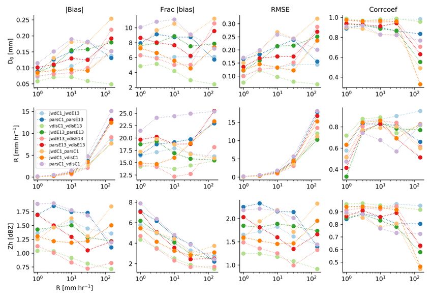
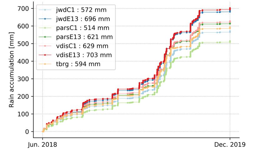
D Wang et al., September 2021, DOE/SC-ARM-TR-275

3.0 Rainfall and DSD Properties at the SGP Site

 3.1 Data Set Overview and Rainfall Characteristics
 In this section, we summarize the precipitation properties as collected by disdrometer and rain gauge
 measurements at the SGP site. The data set was filtered based on processes summarized in Section 2. The
 SGP record considered in this study contains 1,789 5-min DSD measurements meeting the data
 processing criteria. These data were collected from over 513 days during an 18-month period
 (June 2018-December 2019) when six disdrometers were operating. These DSDs are associated with a
 total precipitation that exceeds 500 mm, with an instrument difference varying from 6% to 18% between
 those disdrometers and the rain gauge measurements (Figure 3). The maximum total rainfall accumulation
 among the disdrometers was 703 mm as recorded by the VDIS-E13, which was 36% higher than the
 lowest total precipitation recorded by the LDIS-C1 (514 mm). As noted, those differences are not
 unexpected given the differences in instrument sampling areas, as well as some natural/physical
 variability in intensity or spatial heterogeneity of the rainfall systems. The high wind effects
 (cross-cutting physical and sampling limitations) may contribute to the differences as well.

 Figure 2. Rainfall accumulation collected by six collocated disdrometers and a tipping bucket rain
 gauge from June 20, 2018 to December 30, 2019 at the SGP site.

 Monthly accumulation breakdowns for the six collocated disdrometers are shown in Figure 3a. The
 warmer-season periods show enhanced rainfall amounts (through May to August) from all the
 disdrometers, which is consistent with previous SGP precipitation studies (e.g., Zhang et al. 2017). More
 frequent passages of the convective cloud systems and frontal intrusions during these seasons contribute
 largely to the total accumulations (e.g., Fritsch et al. 1986), especially the organized mesoscale convective
 systems (MCSs). All disdrometers consistently capture a maximum accumulation peaking in August
 (approximately 120 mm over the study period), and slightly reduced rainfall in other warmer season
 months (minimum found in July, approximately 60 mm). Note: while these behaviors are initially
 suggested as reasonable, the limited samples during this 18-month observational period are not intended
 to represent the SGP rainfall annual cycles. For example, year-to-year variability in precipitation over the

 8

D Wang et al., September 2021, DOE/SC-ARM-TR-275

SGP site may be significant, depending partially on the large-scale moisture transport and convergence
(e.g., through low-level jets from the Gulf of Mexico; Helfand and Schubert 1995, Higgins et al. 1997)
and soil moisture (Welty and Zeng 2018).

Similarly, we plot the diurnal cycles of the rainfall accumulation in Figure 3b. A
nocturnal-to-early-morning rainfall maximum is observed by all six units at the site from
0200 UTC-1700 UTC. This behavior is more pronounced during the summertime, as also documented in
previous studies (e.g., Wallace 1975, Dai et al. 1999). This nocturnal precipitation maximum has been
found to be associated with the eastward-propagating convective cloud systems (e.g., MCSs;
Carbone et al. 2002), a reversal of the mountain-plains circulation (Carbone and Tuttle 2008), and an
enhanced moisture transport by low-level jet during nighttime (Berg et al. 2015). Interestingly, the
differences in Figure 3 between the similar types of disdrometers are consistently distributed to each
month of the year and each hour of the day. This behavior suggests that these differences are likely due to
specific instrument calibration issues and/or high wind effects (e.g., unit pairings such as LDIS having
known and relative biases as contingent on sampling relative to prevailing winds, storm motion).

Figure 3. The annual and diurnal cycles of rainfall accumulation collected by six collocated
 disdrometers from June 20, 2018 to December 30, 2019 at the SGP site.

3.2 Summary of the DSD Properties
In Table 2, we summarize the key rainfall parameters and radar quantities from disdrometers breaking
down according to the rainfall rate intensity (for requests for specific parameters, please contact the
instrument mentor). All the instruments show consistent behaviors within each rainfall rate interval in
terms of mean R, D0, Nw, Z, and ZDR. For instance, the mean rainfall rate from each instrument is generally

 9

D Wang et al., September 2021, DOE/SC-ARM-TR-275

within 4.5% of the other instruments. The discrepancies between different disdrometer types are most
pronounced for Nw, which is expected due to the known differences associated with smaller drop
sampling. For example, the LDIS measurements exhibit lower drop concentrations Nw
(~ 4000 mm-3 mm-1) for the lighter rainfall rate bins (R < 1 or 1< R < 10 mm hr-1) compared to the other
types of disdrometers. The VDIS has a higher Nw (~ 8000 mm-3 mm-1) and smaller D0 (2.02 mm) for the
larger rainfall rate bin (R > 30 mm hr-1), which has also been found in previous disdrometer studies
(e.g., Battaglia et al. 2010, Gatlin et al. 2015, Park et al. 2017, Giangrande et al. 2019). Except for Nw, the
LDIS reports slightly higher values for the other DSD and rainfall parameters compared to JWD and
VDIS.

Table 2. A summary of 5-min DSD parameter breakdowns for the number of DSDs, rain rate R,
 median volume drop size D0, normalized DSD intercept parameter Nw, radar reflectivity Z
 and ZDR at S-band wavelengths, filtered according to rainfall rate intervals.

 R # of DSDs [mm/hr] [mm]

 JWD-C1, JWD-E13, LDIS-C1, LDIS-E13, VDIS-C1, VDIS-E13

 30 21, 34, 16, 28, 28, 40 39.8, 44.1, 44.1, 43.0, 43.7, 2.13, 2.23, 2.14, 2.19, 2.02, 2.02
 44.0

 R [mm-3 mm-1] [dBZ] [dB]

 JWD-C1, JWD-E13, LDIS-C1, LDIS-E13, VDIS-C1, VDIS-E13

 30 4542, 5001, 5527, 4643, 7655, 8342 48, 48, 48, 49, 48, 48 1.1, 1.2, 1.2, 1.3, 1.1, 1.1

Figure 4a shows the DSD composite behaviors for all the disdrometers based on the cumulative data set.
This comparison highlights the great agreement between three different types of disdrometers in terms of
their average drop number concentrations, especially within the mid-size drop range for D between 1 mm
and 4 mm. However, sampling differences between different sensors and instrument types are most
pronounced in the smaller and larger raindrop size ranges. The drop number concentration (N) peaks at
the first/second available size bin (centered at 0.36 mm/0.3 mm in D) for the JWD/VDIS. For the LDIS,
the peak of N is located at the fifth-size bin (centered at 0.56 mm in D), with both units suggesting
relative under-sampling of the raindrops at the smaller drop sizes (D < 0.56 mm). Here, these issues may
be influenced by LDIS reduced sensitivity in these drop size ranges (e.g., Tokay et al. 2013). As we
highlight in Figure 4b, this underestimation tends to be more pronounced for higher-rainfall-intensity

 10

D Wang et al., September 2021, DOE/SC-ARM-TR-275

sampling (R > 10 mm/hr). Interestingly, for larger drop sizes (D > 4 mm), an opposite tendency is found.
Here, the LDIS relatively overestimates the number of larger drops. This overestimation of larger drops
lends explanation for the higher relative R and Z estimates as also reported in Table 2. These
discrepancies in sampled DSDs by different disdrometers are nonetheless consistent with previous
disdrometer intercomparison studies at other locations (e.g., Park et al. 2017, Tokay et al. 2013,
Giangrande et al. 2019).

Focusing momentarily on the JWD measurements, especially those collected by JWD-C1, these units
sample the fewest number of large rain drops compared to the other adjacent disdrometers. This may be
partially attributed to the fact JWD has the smallest sampling area among the disdrometer types. In
addition, the background noise, high wind effects, and dead-time corrections may degrade the accuracy of
measuring drop counts using JWD (e.g., Tokay et al. 2003, 2005, Tokay and Bashor 2010). Moreover, a
prominent underestimation of drop number concentration is found at the small drop end of the JWD size
spectra (0.5 mm < D < 1 mm), as compared to LDIS and VDIS (Figure 4a). This underestimation is more
pronounced for the likely deep convective core DSDs having R > 10 mm/hr (Figure 4b). The suggestion
is that the JWD fails to capture the largest portion of small raindrops (e.g., those that would experience
more efficient rainfall evaporation near convective clouds, e.g., Sauvageot and Lacaux 1995,
Atlas and Ulbrich 2000, Tokay et al. 2013). In contrast, the VDIS occasionally report spurious small
drops (e.g., Tokay et al. 2002), primarily during intense convective events (Figure 4b) as related to the
Velcro-type splash guard material around the orifice that becomes less effective as it saturates quickly
with the heavy rainfall. Nevertheless, VDIS performance is consistent with expectations as the most
reliable unit among all.

Figure 4. Averaged drop size distributions for all the measurements (a) and for convective rainfall
 (R > 10 mm hr-1) and stratiform rainfall events (R ≤ 10 mm hr-1), separately (b).

 11

D Wang et al., September 2021, DOE/SC-ARM-TR-275

4.0 Uncertainties in Rainfall and Radar Quantities

 4.1 Biases in Sampling Key Properties
 For statistical comparisons, we calculate the bias, absolute bias, fractional absolute bias, RMSE, and
 correlation coefficient between different disdrometer pairs for key quantity, rainfall (R), as shown in
 Figure 5 and Table 3. Most co-disdrometer (similar instrument type) and cross-disdrometer (different
 instrument types) pairings indicate a good agreement between the various instruments, with a bias within
 +-1 mm hr-1, a |bias| lower than 1.2 mm hr-1, and a fractional |bias| lower than 28%. Among various pairs
 considered, a considerable reduction in bias is found using the same disdrometer type, with the lowest
 biases found for the VDIS pairs (|bias| = 0.97, frac|bias| = 24.1 %, Table 3). The measurements from most
 pairings are also highly correlated (r > 0.9). This confirms these instruments as sampling similar rainfall
 conditions that supersede select known challenges related to the different disdrometer sampling areas and
 other limitations in measuring various drop sizes (e.g., Table 1, Figure 5).

 We also analyze additional results in a similar form for D0 and Z (not shown). One consistent suggestion
 from these additional key parameters is that the non-matching disdrometer pairs exhibit the higher biases
 and the lowest r, with the worst performances found for a particular LDIS-C1 and VDIS-C1 pairing.
 Since the LDIS raindrop sampling is sensitive to prevailing winds and sampling areas, such discrepancy
 from these pairings is not surprising. These issues would be in addition to the spatial inhomogeneity and
 other complexities that might more randomly complicate most disdrometer intercomparisons.

 Figure 5. The Bias, absolute bias (|Bias|), RMSE, Frac |Bias|, correlation coefficient in terms of rainfall
 rate for paired disdrometers.

 12

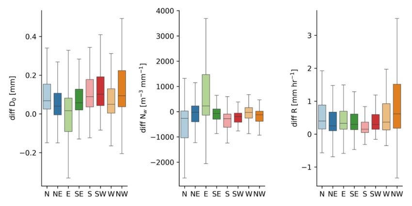
D Wang et al., September 2021, DOE/SC-ARM-TR-275

Table 3. A summary of 5-min DSD parameter breakdowns for the number of DSDs, rain rate R,
 median volume drop size D0, normalized DSD intercept parameter Nw, radar reflectivity Z.

 Fra|Bias| Fra|Bias| Fra|Bias|
 |Bias| [%] RMSE r |Bias| [%] RMSE r |Bias| [%] RMSE r

 D0 [mm] R [mm hr-1] Z [dBZ]
 JWD
 0.10 6.8 0.14 0.98 1.12 23.8 3.51 0.95 1.68 5.5 2.13 0.98
 pair
 VDIS
 0.08 5.4 0.13 0.97 0.97 24.1 3.48 0.89 1.27 4.2 2.11 0.96
 pair
 LDIS
 0.15 10.1 0.23 0.92 1.22 26.4 3.37 0.95 2.07 6.7 2.78 0.96
 pair

Among all comparisons between similar disdrometer types, the LDIS pairs suggest the worst performance
in terms of the D0, R, and Z agreements. It’s worth mentioning that we suspect there is an issue with the
LDIS-E13 unit according to the ARM DQRs. The paired LDIS performance may be impacted by the
LDIS-E13 instrument performance. As suggested prior, even while limiting the potential error sources (as
from spatial variability within the rain systems) by reducing the distance between these disdrometers to
2 meters, discrepancies in DSD sampling may reflect device orientation relative to the prevailing or
storm-relative winds. In Figure 6, we break down the differences between the D0, Nw, and R estimates for
these side-by-side LDISs (LDIS-E13−LDIS-C1) according to surface wind directions measured by the
ARM surface meteorology systems (MET). Because the long axis of LDIS-E13 is north-south, whereas
this axis is east-west for LDIS-C1, it is less surprising that easterly/westerly winds promotes higher Nw for
the LDIS-E13 oriented perpendicular compared to LDIS-C1. With regard to median drop size (D0), the
LDIS-E13 estimates tend to promote more small drops than those from LDIS-C1 when experiencing
easterly/westerly flows, and larger sizing when winds are from the other directions. As an independent
reference, note that the distributions of DSD properties from VDIS are far less influenced by the wind
direction (not shown).

Figure 6. Box-and-whisker plots of the differences of D0, Nw, and R between LDIS-E13 and LDIS-C1
 as a function of wind direction. The middle lines show the median values. The colored boxes
 represent observations inside the 25th to 75th percentile range. The whiskers show the 10th
 and 90th percentile values.

 13

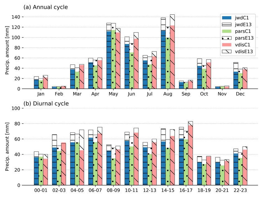
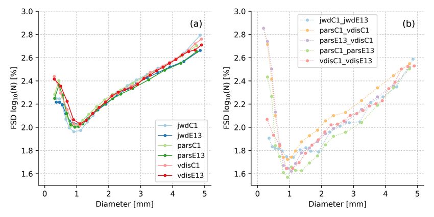
D Wang et al., September 2021, DOE/SC-ARM-TR-275

In Figure 7, we show the biases, RMSE, and correlations between different disdrometer pairs contingent
on different R intervals. Overall, the absolute bias and RMSE increase with increasing rain rate for most
of the pairs in terms of D0 and R. One exception is the VDIS pairs, which show a better performance
overall. The correlation coefficient drops dramatically for the higher rainfall rate range (> 30 mm hr-1)
due to the limited samples in this R bin. Interestingly, the JWD-E13 and VDIS-E13 pair shows a
comparable performance to the VDIS pairs, which may be attributed to previous discussions on the JWD
performing reasonably well for capturing DSD properties, especially for sampling small drops.

Figure 7. The bias, absolute bias (|Bias|), RMSE, Frac |Bias|, r shown as a function of rainfall rate (R)
 when comparing D0, R, and Z between paired disdrometers.

4.2 Reducing Sampling Errors Using Collocated Measurements
All DSD measurements from disdrometers are subject to statistical sampling errors due to the Poisson
distributed fluctuations of the number of samples in each drop size interval. This would extend to the
integrated properties such as rainfall rate and radar reflectivity that are estimated based on these DSD
parameters. In this study, we use the FSD as introduced previously to quantify the instrument sampling
errors following Cao et al. (2008). In Figure 8, we present the FSDs of the rain drop count (N) estimated
using Equation 2 for each unit (Figure 8a), as well as the paired units (Figure 8b) as a function of drop
diameter. The FSDs of N increase considerably with drop diameter when D > 1 mm, with a minimum
FSD of ~ 2 % for D = 1 mm. This behavior suggests an increased sampling error in these size bins, as due
to the under-sampling of the relatively larger raindrops.

 14

D Wang et al., September 2021, DOE/SC-ARM-TR-275

 For drops smaller than 1 mm, the sampling error increases with decreasing drop size for all the units. This
 is because all disdrometers are unable to accurately measure smaller raindrops due to various instrument
 limitations. Perhaps less surprisingly, the FSDs of N agree well for the medium-sized drops between
 different single units. Once again, these instruments show their largest discrepancies for smaller (D < 1.3
 mm) and larger (D > 3 mm) size bins. When considering side-by-side paired disdrometer measurements
 (Figure 8b), we potentially eliminate the errors associated with physical process variations in the rain drop
 behaviors, thus significantly reducing the sampling errors (by 2.5 % for D = 1 mm). Co-located
 disdrometers (all types, pairings) deployed in the field would serve to sizably reduce the statistical
 sampling errors in DSD measurements.

 Figure 8. FSD of the observed drop counts over the bin spectrum. The solid line represents the
 calculation based on a single instrument; the dotted line represents the result from
 side-by-side paired instruments.

5.0 References
 Ackerman, TP, and GM Stokes. 2003. “The atmospheric radiation measurement program.” Physics Today
 56(1): 38, https://doi.org/10.1063/1.1554135

 Atlas, D, and CW Ulbrich. 2000. “An observationally based conceptual model of warm oceanic
 convective rain in the tropics.” Journal of Applied Meteorology and Climatology 39(12): 2165–2181,
 https://doi.org/10.1175/1520-0450(2001)0402.0.CO;2

 Battan, LJ. 1973. Radar Observation of the Atmosphere. University of Chicago Press, Chicago.

 Battaglia, A, E Rustemeier, A Tokay, U Blahak, and C Simmer. 2010. “PARSIVEL snow observations:
 A critical assessment.” Journal of Atmospheric and Oceanic Technology 27(2): 333–344,
 https://doi.org/10.1175/2009JTECHA1332.1

 Bartholomew, MJ. 2016. Impact Disdrometer Instrument Handbook. U.S. Department of Energy.
 DOE/SC-ARM-TR-111.

 15

D Wang et al., September 2021, DOE/SC-ARM-TR-275

Bartholomew, MJ. 2020b. Two-Dimensional Video Disdrometer (VDIS) Instrument Handbook. U.S.
Department of Energy. DOE/SC-ARM-TR-111.

Bartholomew, MJ. 2020a. Laser Disdrometer Instrument Handbook. U.S. Department of Energy.
DOE/SC-ARM-TR-137.

Berg, LK, LD Riihimaki, Y Qian, H Yan, and M Huang. 2015. “The Low-Level Jet over the Southern
Great Plains Determined from Observations and Reanalyses and Its Impact on Moisture Transport.”
Journal of Climate 28(17): 6682–6706, https://doi.org/10.1175/JCLI-D-14-00719.1

Berne, A, and R Uijlenhoet. 2005. “Quantification of the radar reflectivity sampling error in non‐
stationary rain using paired disdrometers.” Geophysical Research Letters 32(19): L19813,
https://doi.org/10.1029/2005GL024030

Bringi, V, and V Chandrasekar. 2001. Polarimetric Doppler Weather Radar: Principles and Applications.
Cambridge University Press, Cambridge, doi:10.1017/CBO9780511541094.

Carbone, RE, and JD Tuttle. 2008. “Rainfall Occurrence in the U.S. Warm Season: The Diurnal Cycle.”
Journal of Climate 21(16): 4132–4146, https://doi.org/10.1175/2008JCLI2275.1

Carbone, RE, JD Tuttle, DA Ahijevych, and SB Trier. 2002. “Inferences of Predictability Associated with
Warm Season Precipitation Episodes.” Journal of the Atmospheric Sciences 59(13): 2033–2056,
https://doi.org/10.1175/1520-0469(2002)0592.0.CO;2

Cao, Q, G Zhang, E Brandes, T Schuur, A Ryzhkov, and K Ikeda. 2008. “Analysis of Video Disdrometer
and Polarimetric Radar Data to Characterize Rain Microphysics in Oklahoma.” Journal of Applied
Meteorology and Climatology 47(8): 2238–2255, https://doi.org/10.1175/2008JAMC1732.1

Dai, A, F Giorgi, and KE Trenberth. 1999. “Observed and model-simulated precipitation diurnal cycle
over the contiguous United States.” Journal of Geophysical Research – Atmospheres
104(D6): 6377–6402, https://doi.org/10.1029/98JD02720

Dolan, B, B Fuchs, SA Rutledge, EA Barnes, and EJ Thompson. 2018. “Primary Modes of Global Drop
Size Distributions.” Journal of the Atmospheric Sciences 75(5): 1453–1476, https://doi.org/10.1175/JAS-
D-17-0242.1

Fritsch, J, R Kane, and C Chelius. 1986. “The Contribution of Mesoscale Convective Weather Systems to
the Warm-Season Precipitation in the United States.” Journal of Applied Meteorology and Climatology
25(10): 1333-1345, https://doi.org/10.1175/1520-0450(1986)0252.0.CO;2

Gage, KS, WL Clark, CR Williams, and A Tokay. 2004. “Determining reflectivity measurement error
from serial measurements using paired disdrometers and profilers.” Geophysical Research Letters
31(23): L23107, https://doi.org/10.1029/2004GL020591

Gatlin, PN, M Thurai, VN Bringi, W Petersen, D Wolff, A Tokay, L Carey, and M Wingo. 2015.
“Searching for large raindrops: A global summary of two‐dimensional video disdrometer observations.”
Journal of Applied Meteorology and Climatology 54(5): 1069–1089, https://doi.org/10.1175/JAMC‐D‐
14‐0089.1

 16

D Wang et al., September 2021, DOE/SC-ARM-TR-275

Gertzman, H, and D Atlas. 1977. “Sampling errors in the measurement of rain and hail parameters.”
Journal of Geophysical Research 82(31): 4955–4966, https://doi.org/10.1029/JC0821031P04955

Giangrande, SE, D Wang, MJ Bartholomew, MP Jensen, DB Mechem, JC Hardin, and R Wood. 2019.
“Midlatitude Oceanic Cloud and Precipitation Properties as Sampled by the ARM Eastern North Atlantic
Observatory.” Journal of Geophysical Research − Atmospheres 124(8): 4741–4760,
https://doi.org/10.1029/2018JD029667

Giangrande, SE, MJ Bartholomew, M Pope, S Collis, and MP Jensen. 2014. “A summary of precipitation
characteristics from the 2006–11 northern Australian wet seasons as revealed by ARM disdrometer
research facilities (Darwin, Australia).” Journal of Applied Meteorology and Climatology
53(5): 1213–1231, https://doi.org/10.1175/JAMC-D-13-0222.1

Gunn, R, and GD Kinzer. 1949. “The Terminal Velocity of Fall for Water Droplets in Stagnant Air.”
Journal of the Atmospheric Sciences 6(4): 243–248, https://doi.org/10.1175/1520-
0469(1949)0062.0.CO;2

Hardin, J, and N Guy. 2017. PyDisdrometer v1.0, https://doi.org/10.5281/zenodo.9991

Helfand, HM, and SD Schubert. 1995. “Climatology of the simulated Great Plains low-level jet and its
contribution to the continental moisture budget of the United States.” Journal of Climate 8(4): 784–806,
https://doi.org/10.1175/1520-0442(1995)00082.0.CO;2

Higgins, RW, Y Yao, ES Yarosh, JE Janowiak, and KC Mo. 1997. “Influence of the Great Plains
low-level jet on summertime precipitation and moisture transport over the central United States.” Journal
of Climate 10(3): 481–507, https://doi.org/10.1175/1520-0442(1997)0102.0.CO;2

Jackson, R, S Collis, V Louf, A Protat, D Wang, S Giangrande, EJ Thompson, B Dolan, SW Powell,
2021. “The development of rainfall retrievals from radar at Darwin.” Atmospheric Measurement
Techniques 14(1): 53–69, https://doi.org/10.5194/amt-14-53-2021

 Joss, J, and A Waldvogel. 1969. “Raindrop size distribution and sampling size errors.” Journal of the
Atmospheric Sciences 26(3): 566−569, https://doi.org/10.1175/1520-0469(1969)026-
0566:RSDASS>2.0.CO;2

Krajewski, WF, A Kruger, C Caracciolo, P Golé, L Barthes, JD Creutin, JY Delahaye, EI Nikolopoulos,
F Ogden, and JP Vinson. 2006. “DEVEX‐disdrometer evaluation experiment: Basic results and
implications for hydrologic studies.” Advances in Water Resources 29(2): 807–814,
https://doi.org/10.1016/j.advwatres.2005.03.018

Leinonen, J. 2014. "High-level interface to T-matrix scattering calculations: architecture, capabilities and
limitations." Optics Express 22(2): 1655−1660, https://doi.org/10.1364/OE.22.001655

Loffler-Mang, M, and J Joss. 2000. “An optical disdrometer for measuring size and velocity of
hydrometeors.” Journal of Atmospheric and Oceanic Technology 17(2): 130–139,
https://doi.org/10.1175/1520-0426(2000)0172.0.CO;2

 17

D Wang et al., September 2021, DOE/SC-ARM-TR-275

Marzuki, HH, M Vonnisa, H Hashiguchi, and H Abubakar. 2018. “Determination of Intraseasonal
Variation of Precipitation Microphysics in the Southern Indian Ocean from Joss–Waldvogel Disdrometer
Observation during the CINDY Field Campaign.” Advances in Atmospheric Sciences 35(1): 1415–1427,
https://doi.org/10.1007/s00376-018-8026-5

Mishchenko, MI, LD Travis, and DW Mackowski. 1996. “T-matrix computations of light scattering by
nonspherical particles: A review.” Journal of Quantitative Spectroscopy and Radiative Transfer
55(5): 535−575, https://doi.org/10.1016/0022-4073(96)00002-7

Montero‐Martínez, G, and F García‐García. 2016. “On the behaviour of raindrop fall speed due to wind.”
Quarterly Journal of the Royal Meteorological Society 142(698): 2013−2020,
https://doi.org/10.1002/qj.2794

Nešpor, V, WF Krajewski, and A Kruger. 2000. “Wind-induced error of raindrop size distribution
measurement using a two-dimensional video disdrometer.” Journal of Atmospheric and Oceanic
Technology 17(11): 1483–1492, https://doi.org/10.1175/1520-0426(2000)0172.0.CO;2

Park, SG, HL Kim, YW Ham, and SH Jung. 2017. “Comparative evaluation of the OTT PARSIVEL2
using a collocated two‐dimensional video disdrometer.” Journal of Atmospheric and Oceanic Technology
34(9): 2059–2082, https://doi.org/10.1175/JTECH-D-16-0256.1

Raupach, TH, and A Berne. 2015. “Correction of raindrop size distributions measured by Parsivel
disdrometers, using a two-dimensional video disdrometer as a reference.” Atmospheric Measurement
Techniques 8(1): 343–365, https://doi.org/10.5194/amt-8-343-2015

Rowland, JR. 1976. “Comparison of two different raindrop disdrometers.” Preprints, 17th Conference on
Radar Meteorology, Seattle, Washington, American Meteorological Society 398–405.

Sauvageot, H, and JP Lacaux. 1995. “The shape of averaged drop size distributions.” Journal of the
Atmospheric Sciences 52(8): 1070–1083, https://doi.org/10.1175/1520-
0469(1995)0522.0.CO;2

Sisterson, DL, RA Peppler, TS Cress, PJ Lamb, and DD Turner. 2016. “The ARM Southern Great Plains
(SGP) Site.” Meteorological Monographs 57: 6.1–6.14, https://doi.org/10.1175/AMSMONOGRAPHS-
D-16-0004.1

Sisterson, DL. 2017. “A Unified Approach for Reporting ARM Measurement Uncertainties Technical
Report.” U.S. Department of Energy. DOE/SC-ARM-17-010.

Schönhuber, M, HE Urban, JPVP Baptista, WL Randeu, and W Riedler. 1997. “Weather radar vs. 2D-
video-distrometer data.” In Weather Radar Technology for Water Resources Management, B. Braga Jr.
and O. Massambani, Eds., UNESCO Press, pp. 159−171.

Schuur, TJ, AV Ryzhkov, DS Zrnić, and M Schönhuber. 2001. “Drop Size Distributions Measured by a
2D Video Disdrometer: Comparison with Dual-Polarization Radar Data.” Journal of Applied Meteorology
and Climatology 40(6): 1019–1034, https://doi.org/10.1175/1520-
0450(2001)0402.0.CO;2

 18