Drought propagation and construction of a comprehensive drought index based on the Soil and Water Assessment Tool (SWAT) and empirical Kendall ...
←
→
Page content transcription
If your browser does not render page correctly, please read the page content below
Nat. Hazards Earth Syst. Sci., 21, 1323–1335, 2021
https://doi.org/10.5194/nhess-21-1323-2021
© Author(s) 2021. This work is distributed under
the Creative Commons Attribution 4.0 License.

Drought propagation and construction of a comprehensive
drought index based on the Soil and Water Assessment Tool
(SWAT) and empirical Kendall distribution function (KC0 ):
a case study for the Jinta River basin in northwestern China
Zheng Liang1,2 , Xiaoling Su1,2 , and Kai Feng1,2
1 College
        of Water Resources and Architectural Engineering, Northwest A & F University, Yangling 712100, China
2 KeyLaboratory for Agricultural Soil and Water Engineering in Arid Area of Ministry of Education,
Northwest A & F University, Yangling 712100, China

Correspondence: Xiaoling Su (xiaolingsu@nwafu.edu.cn)

Received: 22 July 2020 – Discussion started: 25 August 2020
Revised: 19 January 2021 – Accepted: 24 March 2021 – Published: 30 April 2021

Abstract. Monitoring drought and mastering the laws of           in the northern and low in the southern regions. MAHDI
drought propagation are the basis for regional drought pre-      proved to be acceptable in that it was consistent with histor-
vention and resistance. Multivariate drought indicators con-     ical drought records, could catch drought conditions charac-
sidering meteorological, agricultural and hydrological infor-    terized by univariate drought indexes, and capture the occur-
mation may fully describe drought conditions. However, se-       rence and end of droughts. Nevertheless, its ability to charac-
ries of hydrological variables in cold and arid regions that     terize mild and moderate droughts was stronger than severe
are too short or missing make it difficult to monitor drought.   droughts. In addition, the comprehensive drought conditions
This paper proposed a method combining Soil and Water As-        showed insignificant aggravating trends in spring and sum-
sessment Tool (SWAT) and empirical Kendall distribution          mer and showed insignificant alleviating trends in autumn
function (KC0 ) for drought monitoring. The SWAT model,          and winter and at annual scales. The results provided theo-
based on the principle of runoff formation, was used to sim-     retical support for the drought monitoring in the Jinta River
ulate the hydrological variables of the drought evolution pro-   basin. This method provided the possibility for drought mon-
cess. Three univariate drought indexes, namely meteorologi-      itoring in other watersheds lacking measured data.
cal drought (standardized precipitation evapotranspiration in-
dex; SPEI), agricultural drought (standardized soil moisture
index; SSI) and hydrological drought (standardized stream-
flow drought index; SDI), were constructed using a para-
metric or non-parametric method to analyze the propagation       1   Introduction
time from meteorological drought to agricultural drought and
hydrological drought. The KC0 was used to build a multi-         According to the fifth evaluation report of the Intergovern-
variable comprehensive meteorology–agriculture–hydrology         mental Panel on Climate Change (IPCC), climate change
drought index (MAHDI) that integrated meteorological, agri-      characterized by temperature rise is the main concern of
cultural and hydrological drought to analyze the characteris-    the global change in the past half-century with the most
tics of a comprehensive drought evolution. The Jinta River       rapid warming in the mid-latitudes of the Northern Hemi-
in the inland basin of northwestern China was used as the        sphere (IPCC, 2018; Ji et al., 2014). The arid inland river
study area. The results showed that agricultural and hydro-      basins of China are mainly located in the hinterland of the
logical drought had a seasonal lag time from meteorologi-        Eurasian continent in the mid-latitudes and are very sensitive
cal drought. The degree of drought in this basin was high        to global climate change. Therefore, it is particularly impor-

Published by Copernicus Publications on behalf of the European Geosciences Union.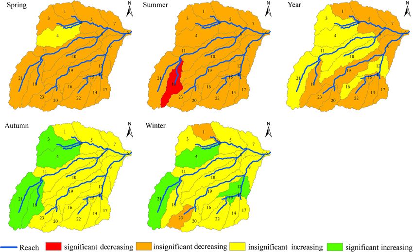
1324                             Z. Liang et al.: Drought propagation and construction of a comprehensive drought index

tant to study the drought conditions of the inland river basins        With the deepening of drought research, the insufficiency
of China under the prevailing climate change scenario.              of univariate drought indexes has gradually emerged. Be-
   Drought is a dynamic creeping phenomenon (Oikonomou              cause drought characteristics are usually interrelated, tradi-
et al., 2019; Ahmadi and Moradkhani, 2019); however,                tional drought research based on univariate frequency analy-
there is no precise definition for the differences in               sis can hardly reflect the multi-dimensional effects of drought
hydro-meteorological variables and socioeconomic elements           on society. Therefore, it is necessary to develop a compre-
(Mishra and Singh, 2010). Generally, the droughts are di-           hensive drought index integrating multiple variables related
vided into four categories (Heim, 2002): (i) meteorological         to drought. Keyantash and Dracup (2004) use principal com-
drought, referring to a period of time with a lack of precipi-      ponent analysis (PCA) to extract dominant drought variables
tation (Mishra and Singh, 2010; Dai, 2011), (ii) agricultural       to develop an aggregate drought index (ADI) for comprehen-
drought, referring to a period with low soil water hinder-          sive drought features (Rajsekhar et al., 2015). However, this
ing crop growth and reducing grain yield (Crow et al., 2012;        method is a linear combination of related variables which
Panu and Sharma, 2002), (iii) hydrological drought, referring       could not reveal its nonlinear structural characteristics. The
to a deficit in streamflow or groundwater resources (Cam-           copula function can connect different marginal distributions
malleri et al., 2016), and (iv) socioeconomic drought, refer-       and consider the correlation between them. It is one of the
ring to a phenomenon that water shortage affects production,        most commonly used connection methods at present and has
consumption and other socioeconomic activities. There is a          been widely used in the field of hydrometeorology (Hao
close relationship among the various droughts. Insufficient         and AghaKouchak, 2013). For example, the joint drought
precipitation for a long time leads to meteorological drought.      index (JDI) is constructed by copula using joint accumu-
When this situation lasts for a long period of time, the soil       lated distribution of the runoff and precipitation (Kao and
water content decreases, which leads to a reduction in crop         Govindaraju, 2010). Guo et al. (2019) use copula to pro-
yield, resulting in agricultural drought. Insufficient precipita-   pose an improved multivariate standardized reliability and
tion for a long period of time also causes a significant drop       resilience index (IMARRI) to fully appraise the dynamic risk
in surface water and groundwater, resulting in hydrological         of socioeconomic drought. Wang et al. (2020) construct a
drought. When all these three types of drought adversely af-        standardized precipitation evapotranspiration streamflow in-
fect social production and economic development, socioeco-          dex (SPESI) based on copula to comprehensively display
nomic drought occurs.                                               characteristics of meteorological and hydrological drought.
   Drought index is an important indicator to characterize and      Nevertheless, the limitation of the copula function is re-
measure the degree of drought, and it can be used to monitor,       flected when connecting three or more drought indicators
evaluate and study the development of drought. For exam-            (Hao and Singh, 2013; Kao and Govindaraju, 2008, 2010),
ple, the standardized precipitation index (SPI) (McKee et al.,      and this phenomenon is generally called “curse of dimen-
1993) and the standardized precipitation evapotranspiration         sionality” (Hao and Singh, 2013). To overcome this limita-
index (SPEI) (Vicente-Serrano et al., 2010) are commonly            tion, this study applied empirical Kendall distribution func-
used as meteorological drought indexes (Vicente-Serrano et          tion (KC0 ) to construct a new comprehensive drought indica-
al., 2012). The hydrological drought indexes are usually gen-       tor by combining precipitation, evapotranspiration, soil water
erated using streamflow, such as the streamflow drought in-         and streamflow. The KC0 is obtained by Nelsen (2006), which
dex (SDI; Nalbantis and Tsakiris, 2008) and the standard-           is based on the generation function of the Archimedean cop-
ized runoff index (SRI; Shukla and Wood, 2008). The soil            ula function family. It is a probability integral transformation
water content is the main variable to calculate the agricul-        method and can transform multidimensional variable infor-
tural drought index, for instance, the crop water stress index      mation into single-dimensional variable information (Hao et
(Jackson et al., 1988) and the standardized soil moisture in-       al., 2017).
dex (Mishra et al., 2015). Calculation of the drought index            The Jinta River basin (JRB) is a tributary basin of the
requires a long time series of drought variables. However, the      Shiyang River basin (SRB) located in a climate-sensitive
scarcity of measured data is a major problem in the process         area (Wei et al., 2020). Therefore, it is important to study
of drought index construction. Therefore, to derive hydro-          further drought conditions in the basin under the influence
logical datasets, indirect means have been attempted, such as       of climate change. The description of drought conditions
the watershed hydrological model. A recent study carried out        is based on the construction of a drought index, which is
by Dash et al. (2019) apply the Soil and Water Assessment           limited by the shortage of measured data. In addition, the
Tool (SWAT) hydrological model to simulate the soil mois-           construction of a comprehensive drought index should re-
ture data and develop a soil moisture stress index (SMSI) for       flect the drought situation comprehensively. In this paper,
agricultural drought analysis. Further, Zhang et al. (2017a)        the univariate drought indexes (SDI, SSI and SPEI) estab-
adopt the variable infiltration capacity (VIC) hydrological         lished by measuring precipitation, streamflow, soil water and
model to monitor soil moisture drought and construct a sea-         evapotranspiration simulated by the SWAT model (Arnold et
sonal forecasting framework subsequently.                           al., 1998; Zhang et al., 2010) explored the propagation time
                                                                    from meteorological drought to hydrological and agricultural

Nat. Hazards Earth Syst. Sci., 21, 1323–1335, 2021                                 https://doi.org/10.5194/nhess-21-1323-2021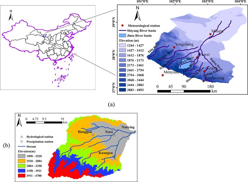
Z. Liang et al.: Drought propagation and construction of a comprehensive drought index                                                    1325

Figure 1. Basic information about the Jinta River basin. (a) The geographic location of the Jinta River in northwestern China; (b) precipitation
and hydrological stations in the Jinta River basin.

drought. A new meteorology–agriculture–hydrology drought                  The terrain of the JRB is higher in the south and lower in
index (MAHDI) was developed using the empirical Kendall                   the north, sloping from southwest to northeast. The altitude
distribution function based on the differences between pre-               ranges from 1890 to 4780 m, with an average altitude of
cipitation and evapotranspiration, streamflow, and soil water.            3000 m (Fig. 1b). The annual precipitation in the basin ranges
MAHDI was also used to estimate the spatial distribution of               from 200 to 500 mm, and the annual evaporation is about
the temporal tendency in different seasons. The specific ob-              700–1200 mm.
jectives are (i) to investigate the propagation time character-
istics from meteorological drought to hydrological and agri-              2.2    Data sources
cultural drought; (ii) to validate the applicability of MAHDI
by comparing it with historical drought events and univariate             A digital elevation model (DEM) with a spatial resolution of
drought indexes (SDI, SSI and SPEI); and (iii) to estimate the            30 m provided by the Geospatial Data Cloud site, Computer
spatial distribution of MAHDI’s temporal tendency in differ-              Network Information Center, Chinese Academy of Sciences
ent seasons.                                                              (http://www.gscloud.cn, last access: 15 June 2020), was used
                                                                          for watershed delineation. The digital soil map was obtained
                                                                          from the Harmonized World Soil Database (HWSD, ver-
2     Materials and methods                                               sion 1.1) developed by the Food and Agricultural Organi-
                                                                          zation of the United Nations (FAO–UN). The map provided
2.1    Study area                                                         data for 5000 soil types containing two soil layers’ worth of
                                                                          information (0–30 and 30–100 cm depth). The land-use data
The Jinta River basin (JRB) with an area of 841 km2 orig-                 (30 m × 30 m) were derived from the satellite remote sens-
inates in the Qilian Mountains and is a tributary of the                  ing image data of Landsat Thematic Mapper (TM) provided
Shiyang River basin located in Gansu Province, China (see                 by the Geographical Information Monitoring Cloud Platform
Fig. 1). It is bounded between 37◦ 020 and 39◦ 170 N and                  (http://www.dsac.cn/DataProduct, last access: 18 June 2020).
100◦ 570 and 104◦ 120 E. The JRB is located in the middle of              The observed climatic information of precipitation, maxi-
the eight subbasins, adjacent to the Zamu River in the east               mum air temperature, minimum air temperature, wind speed
and to the Xiying River in the west, as shown in Fig. 1a.                 and relative humidity was obtained from six meteorologi-

https://doi.org/10.5194/nhess-21-1323-2021                                        Nat. Hazards Earth Syst. Sci., 21, 1323–1335, 2021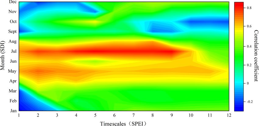
1326                               Z. Liang et al.: Drought propagation and construction of a comprehensive drought index

cal stations shown in Fig. 1a and three precipitation sta-            in the form of base flow calculated by groundwater storage
tions shown in Fig. 1b. The monthly river discharge data              and continuous runoff in the dry season.
for the model calibration and validation were obtained from
the Nanying hydrological station at the Hydrology and Water           2.4     Univariate drought index
Resources Bureau of Gansu Province for the period of 1986–
2012.                                                                 A drought index contains a clear physical mechanism
                                                                      (Keyantash and Dracup, 2002) and is the main tool for the
2.3    SWAT model                                                     quantitative analysis of drought characteristics. In addition,
                                                                      it can monitor the situation of the start time, the end time,
The SWAT model developed by the Agricultural Re-                      duration, intensity and spatial range of drought. Therefore,
search Service of the United States Department of Agri-               the construction of the drought index is the basis of drought
culture (USDA-ARS) is a continuous-time, semi-distributed             research. The differences of precipitation and evapotranspi-
and physics-based water quality model (Arnold et al., 1998;           ration (P –ET), soil moisture (SM) and streamflow (D) sim-
Gassman et al., 2014; Romagnoli et al., 2017) for simulat-            ulated by the SWAT model were used to construct a me-
ing hydrological cycle, plant growth cycle and transportation         teorological drought index (SPEI), agricultural drought in-
of sediments (Arnold et al., 1998; Pyo et al., 2019; Stefani-         dex (SSI) and hydrological drought index (SDI) for differ-
dis et al., 2018; Wu et al., 2011). The SWAT model delin-             ent timescales (1, 3 and 12 months) using parametric or non-
eates a catchment into subbasins based on the stream net-             parametric methods.
work and topography and subsequently into hydrological re-
sponse units (HRUs) representing different combinations of            2.4.1    Parametric methods
soil types, land use and slope. The simulation calculation of
soil effective moisture content, surface runoff, nitrogen con-        The monthly sequence for each drought variable was fitted
tent and sediment yield are carried out for each of the HRUs.         one by one by selecting an appropriate distribution func-
The hydrological part of the model is based on the water bal-         tion. The maximum likelihood method was applied to esti-
ance equation in the soil profile with processes, including           mate the relevant parameters of the distribution function, the
precipitation, surface runoff, infiltration, evapotranspiration,      Kolmogorov–Smirnov (K–S) test was used to test the fitting
lateral flow, percolation and groundwater flow (Arnold et al.,        priority, and the Akaike’s information criterion (AIC) was
1998; Kiniry et al., 2005).                                           used to select the optimal fitting function. The cumulative
                                                                      probability distribution for each drought variable was then
              t
              X                                                      transformed into the standard normal distribution. Finally,
SWt = SW0 +         Rday,i − Qsurf,i − Eα,i − wseep,i − Qgw,i , (1)
              i=1
                                                                      the inverse function of the normal distribution was used to
                                                                      calculate the drought index.
where SWt is the final soil water content at time pe-
riod t (mm), SW0 is the initial soil water content (mm), t is           i. The distributions selected in this study include gamma
the time (number of days), Rdays,i is the amount of rainfall               distribution, log-normal distribution, Weibull distribu-
on ith day (mm), Qsurf,i is the amount of surface runoff on                tion, normal distribution and logistic distribution. As-
ith day (mm), Eα,i is the amount of evapotranspiration on                  suming that each distribution was suitable for the related
ith day (mm), wseep,i is the amount of water giving recharge               drought variable series of each timescale, the maximum
to groundwater from the soil profile on ith day (mm), and                  likelihood method was used to fit the parameter estima-
Qgw,i is the amount of return flow on ith day (mm).                        tion. For a probability density function f (x, θ ), θ is the
   The runoff simulation of the watershed mainly consists of               parameter to be estimated, and X1 , X2 , X3 , . . . , Xn is
evapotranspiration, surface runoff, soil water and groundwa-               a sample from the population. If x1 , x2 , x3 , . . . , xn is
ter. The SWAT model has two main methods for estimat-                      the sample value, the steps of the maximum likelihood
ing surface runoff, which are predicted by the Soil Con-                   method are as follows.
servation Service (SCS) curve (Bouraoui et al., 2005). The
channel routing uses the Muskingum method or the variable                     a. Construct the likelihood function of the sample.
storage coefficient model, including the migration of water,                                                             n
                                                                                                                         Y
sediment, nutrients and pesticides in the river network. The                     L(θ ) = L (x1 , x2 , . . ., xn ; θ) =         f (xi , θ )   (2)
simultaneous calculation of reservoir confluence is also re-                                                             i=1
quired. Evapotranspiration in the SWAT model refers to the
process of surface water transforming into water vapor, in-                   b. The log-likelihood function is given as follows:
cluding water evaporation, transpiration and sublimation re-                                  n
                                                                                              X
tained by tree crowns, as well as soil water evaporation. A                      ln L(θ ) =         f (xi , θ ) .                            (3)
part of the soil water is absorbed by plants or lost by tran-                                 i=1
spiration, a part of it supplies the groundwater, and the other
part forms runoff on the surface. Groundwater runoff exists

Nat. Hazards Earth Syst. Sci., 21, 1323–1335, 2021                                     https://doi.org/10.5194/nhess-21-1323-2021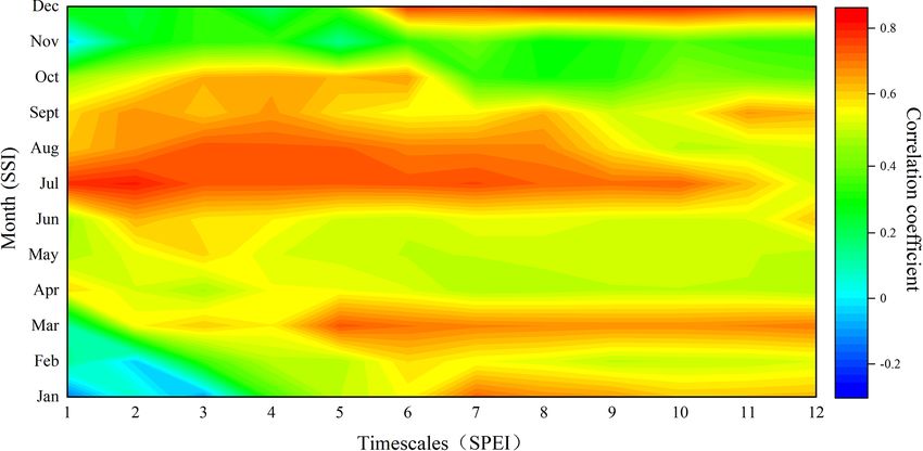
Z. Liang et al.: Drought propagation and construction of a comprehensive drought index                                        1327

     c. Take the derivative of the parameter θ in Eq. (3) and      2.4.2    Non-parametric method
        make the derivative value 0:
                                                                   If the four theoretical distributions for a certain drought vari-
         d ln L(θ )
                    = 0.                                    (4)    able could not pass the K–S test in the process of building
             dθ                                                    a parametric drought index, the non-parametric method was
     d. Solve the likelihood equation to get the maximum           used to build the drought index.
        likelihood estimate θ̂ for the parameter θ.                             i − 0.44
                                                                   Pnonp (xi ) =          ,                                   (8)
 ii. The Kolmogorov–Smirnov (K–S) test is suitable for                          n + 0.12
     testing the goodness-of-fit of a dataset for most of the      where n is the length of the sequence, i is the order when
     probability distributions regardless of the sample size       the sequence of variables is ascending, and Pnonp is the em-
     by comparing the cumulative sample distribution with          pirical cumulative probability. The inverse standardization of
     the cumulative distribution function specified by the         the empirical cumulative probability is the non-parametric
     null hypothesis. If the absolute value of the difference      drought index expressed as follows:
     is within the specified range, the sample obeys the as-
                                                                   DInonp = ∅−1 Pnonp ,

                                                                                                                              (9)
     sumed theoretical distribution. We made H0 the sample
     obeying the theoretical distribution, and H1 indicated        where DInonp is the non-parametric drought index value.
     that the sample did not follow the theoretical distribu-
     tion. The statistic D is constructed as follows:              2.5     Trivariate drought index

    D = max |F1 (x) − F2 (x)| ,                             (5)    The Kendall distribution function is obtained from the gen-
                                                                   eration function of the Archimedean copula function family.
    where F1 (x) represents the cumulative distribution of         It is a probability integral transformation method (Nelsen,
    samples, and F2 (x) represents the theoretical distribu-       2006) and can convert multidimensional variable informa-
    tion. At the selected significance level of α (α = 0.05),      tion into one-dimensional variable information. As some
    if D > D(n, α) (n is the sample size), the H0 is rejected,     copula functions may not have the analytic expression of
    and H1 is accepted; otherwise, H0 is accepted, and H1 is       the Kendall distribution function, this study used a non-
    rejected.                                                      parametric method to construct the empirical Kendall distri-
iii. Akaike’s information criterion (AIC) is a standard to         bution function (Nelsen et al., 2003; Hao et al., 2017) ex-
     measure the goodness-of-fit of the statistical model          pressed as follows:
     founded and developed by Japanese statistician Akaike.                      n2
                                                                   KC0 = Ptri = ,                                             (10)
     It weighs the complexity of the estimated model and the                      n
     goodness of the model fitting data and is given as fol-       where n2 is the number of samples satisfying C 0 (i/n, j/n,
     lows:                                                         k/n) ≤ p (C 0 is the empirical copula function), n is the total
    AIC = 2m − ln L,                                        (6)    number of samples, and Ptri is the three-dimensional cumu-
                                                                   lative probability. The express of empirical copula is given as
    where m is the number of parameters estimated by the           follows (Hao et al., 2017):
    distribution function, and L is the maximum likelihood
                                                                     0 i j k          n1
    function value. As increasing the number of free param-        C      , ,      = ,                                        (11)
                                                                         n n n         n
    eters improves the goodness of fitting, AIC encourages
    the goodness of data fitting but tries to avoid overfitting.   where n1 is the number of the samples (xm , ym , zm ) satisfying
    Therefore, the priority model should be the one with the       (xm ≤ x(i) and ym ≤ y(j ) and zm ≤ z(k) ) and 1 ≤ m ≤ n.
    lowest AIC value. A lower AIC value indicates a better            The empirical Kendall distribution function was used to
    fit.                                                           join the three drought-related variables to obtain a trivariate
                                                                   drought indicator by inverse standardization:
    According to the AIC, the optimal theoretical distri-
    bution was selected. The inverse standardized value of         MAHDI = ∅−1 (Ptri ) ,                                       (12)
    the theoretical distribution value corresponding to each
    drought variable was taken as the parametric drought           where MAHDI is the trivariate drought index value.
    index:
                                                                   3     Results and discussion
    DIp = ∅−1 (P ),                                         (7)

    where DIp is the parametric drought index value, ∅ is          3.1     SWAT model calibration and validation
    the standard normal distribution function, and P is the
                                                                   In order to calibrate and validate the runoff-related pa-
    theoretical cumulative probability.
                                                                   rameters, we applied the SWAT calibration and uncertainty

https://doi.org/10.5194/nhess-21-1323-2021                                  Nat. Hazards Earth Syst. Sci., 21, 1323–1335, 2021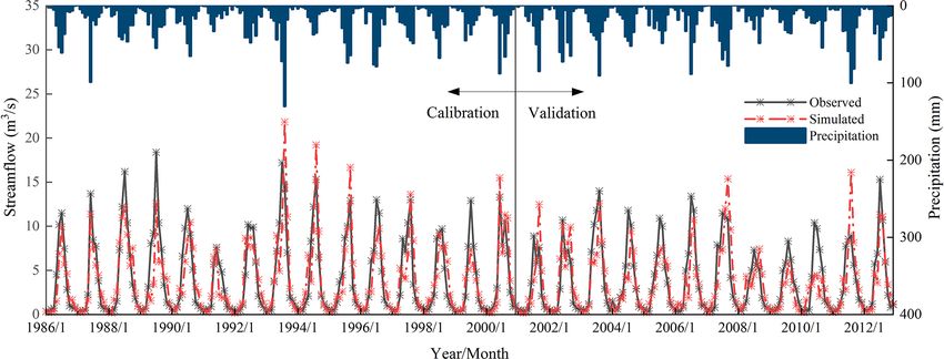
1328                            Z. Liang et al.: Drought propagation and construction of a comprehensive drought index

programs (SWAT-CUPs). The calibration period was taken            timescales also reflected the propagation time from meteo-
as 1986–2000, and the validation period was taken as 2001–        rological drought to agricultural drought. We can mention
2012. In addition, a warm-up period of 1984–1986 was con-         subbasin no. 6 where the hydrological station is located as an
sidered to minimize the uncertainty caused by the initial en-     example.
vironment of the model (Zhang et al., 2019). In the SWAT-            Figure 3 shows the correlation coefficients between
CUPs, the sequential uncertainty fitting version 2 (SUFI-2)       monthly SDI and SPEI with various timescales at subbasin
algorithm (Abbaspour et al., 2007) was chosen for parameter       no. 6. High correlation coefficients (> 0.7) of SDI and SPEI
sensitivity and model uncertainty analysis (Abbaspour et al.,     were observed for spring and summer with the timescales
2015).                                                            from 2 to 9 months. Low correlation coefficients (> 0.4)
    Table 1 shows the top four sensitivity parameters of the      were observed for autumn and winter with about a 6–9 month
JRB and their initial and fitted values. The CN2, the com-        scale. The lag time in spring and summer was more obvi-
prehensive response of the underlying surface characteristics,    ous, showing certain seasonal characteristics, whereas the lag
was the most sensitive parameter in the hydrological process.     time in autumn and winter had inconspicuous seasonal char-
The value of CN2 was calibrated to 70.51–95.03 for different      acteristics. A reasonable explanation for this phenomenon
land-use types. In order, the next sensitivity parameters were    might be more sources of recharge (rainfall and iceberg
SOL_AWC, TLAPS and SOL_K. Among them, SOL_AWC                     snowmelt) in spring and summer, while groundwater was
and SOL_K are soil-related sensitivity parameters, and their      the only source of recharging the river in autumn and win-
fitted values were 0.008 and 99.65, respectively. The TLAPS       ter, which was related to the water stored during spring and
is a parameter related to temperature, and its optimal value      summer.
was 2.83.                                                            Similarly, Fig. 4 depicts the propagation time from mete-
    Uncertainty of the model was adjudged on the basis of         orological drought to agricultural drought at subbasin no. 6,
P -factor and R-factor indicators (Abbaspour et al., 2007).       which also shows an obvious seasonal characteristic. In sum-
When the P factor > 0.7 and R factor < 1.5, the uncertainty       mer, the lag time was approximately concentrated over 2
of the model was considered as acceptable, and the param-         months with a correlation coefficient value higher than 0.8,
eter ranges were taken as the calibrated parameters. Table 2      while the response time in other seasons was longer. The
shows that two indicators are in the acceptable range, with       propagation time from meteorological drought to agricultural
a P factor of 0.72 and an R factor of 0.65. To measure the        drought was, therefore, the shortest in summer. This may be
model performance, we selected the coefficient of determina-      the result of high soil moisture due to high rainfall during the
tion (R 2 ) and the Nash–Sutcliffe simulation efficiency (ENS )   season. The propagation time in spring was 3 months longer
(Table 2). The simulation results showed that the R 2 and ENS     than that in summer, which may be because of the potential
in the JRB were 0.76 and 0.75, respectively, for the calibra-     influence of snowmelt. In the autumn and winter, there was
tion period and 0.73 and 0.72, respectively, for the validation   a longer lag time (6–12 months) in responding to the me-
period. Figure 2 shows the plots for the simulated monthly        teorological drought, possibly due to the infiltration of soil
streamflow against the observations. The figure indicated that    water during the preceding months. Compared with spring
the simulated and observed monthly streamflow were in good        and summer, the evaporation rate of soil water in autumn and
agreement with the period considered, and their changes fol-      winter was slower than that in spring and summer, which pro-
lowed the precipitation. Overall, the model performance was       longed the time when the soil water content reduced to that
satisfactory for subsequent analysis.                             of the threshold for agricultural drought. This made the agri-
                                                                  cultural drought lag behind the meteorological drought for a
3.2     Drought characterization                                  long time.
                                                                     Compared to Fig. 3, Fig. 4 is more precise in showing
The SPEI, SSI, SDI and MAHDI were applied to all sub-             that the propagation time from meteorological drought to
basins for different timescales. For calculating the four in-     agricultural drought increases with a decrease in tempera-
dexes, precipitation, evapotranspiration, soil moisture and       ture and precipitation, and there is a clear gap between dif-
streamflow, data from 1986 to 2012 were adopted in this           ferent seasons. However, the time of hydrological drought
study. Thresholds of the indexes were divided according to        lagging behind the meteorological drought was not obvious.
the SPI (McKee et al., 1993).                                     The distribution of glaciers in the upper reaches of the Jinta
                                                                  River and the significantly longer time of soil water infil-
3.2.1    The propagation time from meteorological                 tration than that of confluence formation might made the
         drought to hydrological and agricultural drought         propagation time from meteorological drought to agricul-
                                                                  tural drought more obvious in different seasons compared to
To study the propagation time from meteorological drought         the propagation time from meteorological drought to hydro-
to hydrological drought, the relationships between the SDI        logical drought. Studying the lag time of different types of
and the SPEI with various timescales were explored. Sim-          droughts from meteorological droughts was helpful in pre-
ilarly, the relationship between SSI and SPEI on different        dicting other droughts using meteorological drought in the

Nat. Hazards Earth Syst. Sci., 21, 1323–1335, 2021                               https://doi.org/10.5194/nhess-21-1323-2021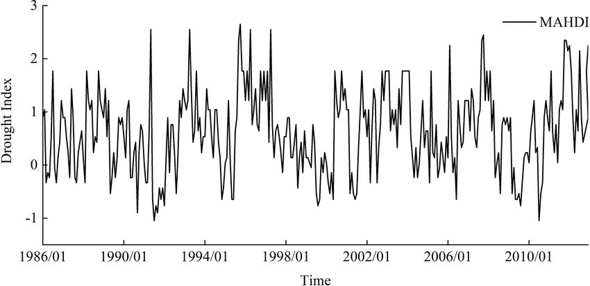
Z. Liang et al.: Drought propagation and construction of a comprehensive drought index 1329
Table 1. Sensitivity analysis and final value range of parameters in Jinta River basin.
Parameters Meaning of parameter Initial Fitted value Method t stat p value
range
CN2∗ SCS runoff curve number for moisture condition II 35–98 70.51–95.03 Replace 43.10 < 0.01
SOL_AWC Available water capacity of the soil layer 0–1 0.008 Replace 38.69 < 0.01
TLAPS Temperature lapse rate −10–10 2.83 Replace −7.72 < 0.01
SOL_K Saturated hydraulic conductivity 0–2000 99.65 Replace 5.04 < 0.01
Note that as the CN2 of different land-use types was calibrated separately, a range of the optimal CN2 values was provided.
Figure 2. Simulated and observed monthly streamflow series relative to precipitation (P ) during the calibration and validation periods in
the JRB.
Table 2. Model performance in monthly streamflow in JRB. cal, agricultural and hydrological drought was obtained. The
monthly change in MAHDI series in sub-watershed no. 6
Indicators P factor R factor R2 ENS from 1986 to 2012 was plotted, as shown in Fig. 5. It can
Calibration period (1986–2000) 0.72 0.65 0.76 0.75 be seen from the figure that 1991, July 1999–May 2000,
Validation period (2001–2012) – – 0.73 0.72 November 1994–January 1995, 2009 and July 2010 were the
drought months. According to the China Meteorological Dis-
aster Dictionary: Gansu Volume, the area was hot and less
absence of measured data and may provide a theoretical ba- rainy in 1991, and continuous drought occurred in summer
sis for drought prevention. and autumn; in 1994–1995, the region suffered from continu-
Both drought propagation and the construction of a com- ous drought in winter and spring; and in 1999, the region suf-
prehensive drought index were based on the data output fered from severe drought in autumn and winter, which were
by the SWAT hydrological model. Drought propagation de- consistent with the drought events described by MAHDI. Ac-
scribed the response relationship between different types of cording to the “Water Resources Bulletin of Gansu Province
drought based on the lag time from agricultural drought and in 2009”, the area had slightly less annual precipitation and
hydrological drought to meteorological drought. The goal in higher temperatures. MAHDI also captured the drought in
the construction of the comprehensive drought index was to this year. Above all, MAHDI can be used to detect the occur-
combine different types of drought indexes and include the rence and development of drought.
lag time from agricultural drought and hydrological drought To analyze the distribution of different droughts and the
to meteorological drought. It reflected the drought state when applicability of MAHDI, the year 1999 was selected for anal-
only one or two kinds of drought occur and could be used to ysis. The spatial distribution of SDI, SSI, SPEI and MAHDI
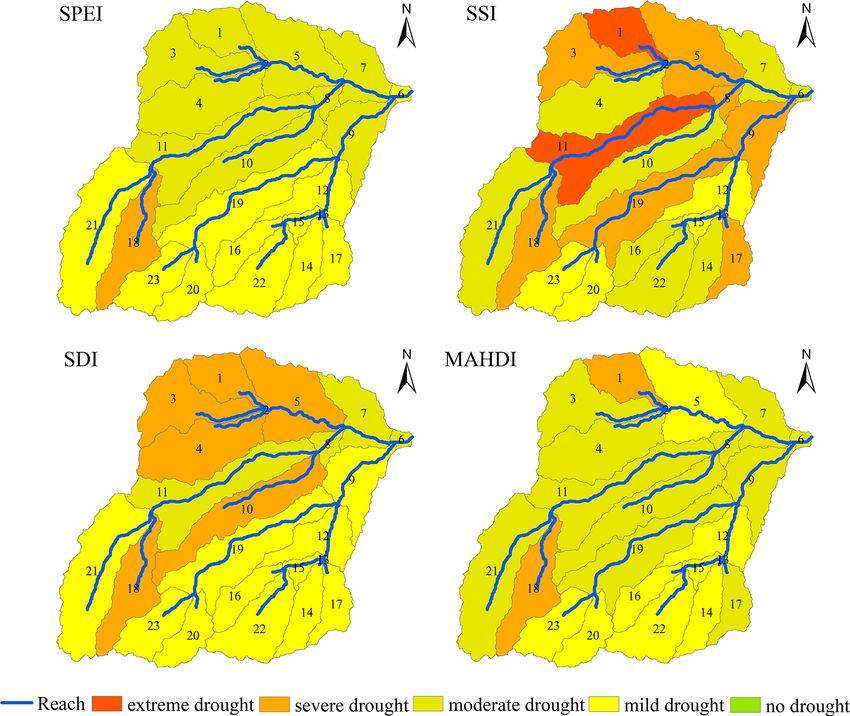
describe the characteristics of drought. for the year 1999 is shown in Fig. 6. For SDI, severe drought
was distributed in subbasin nos. 1–5, 10 and 18. Moderate
3.2.2 Applicability analysis of MAHDI drought was observed in subbasin nos. 6–8 and 11, and mild
drought was observed in the rest of the subbasins. For SSI,
Using the empirical Kendall function to combine the uni- extreme drought was distributed in subbasin nos. 1, 2 and 11,
variate drought indexes, a comprehensive drought index, severe drought was located in subbasin nos. 3, 5, 8, 9 and 17–
MAHDI, that can simultaneously characterize meteorologi-
https://doi.org/10.5194/nhess-21-1323-2021 Nat. Hazards Earth Syst. Sci., 21, 1323–1335, 20211330 Z. Liang et al.: Drought propagation and construction of a comprehensive drought index
Figure 3. The correlation coefficients between monthly SDI and SPEI with different timescales at subbasin no. 6.
Figure 4. The correlation coefficients between monthly SSI and SPEI with different timescales at subbasin no. 6.
vere drought was located in subbasin nos. 1, 2 and 18, mild
drought was distributed in subbasin nos. 5, 12–16, 20 and 22–
23, and moderate drought was located in the rest of the sub-
basins. In conclusion, the drought in the northern part of the
basin was stronger than that in the southern part of the basin.
Different drought indexes showed different degrees of
drought severity. For univariate drought indexes, SSI showed
the highest degree of drought, followed by SDI, and SPEI
showed the lowest degree of drought. SPEI reflected the low-
est degree of meteorological drought, which was similar to
that described by the Thornthwaite aridity index (AI) con-
Figure 5. Monthly scale MAHDI sequence at subbasin no. 6.
structed by Zhang et al. (2017b) using rainfall and poten-
tial evapotranspiration. As rainfall and temperature were the
core elements of SPEI, the meteorological drought was al-
19, moderate drought was observed in subbasin nos. 4, 6, leviated (Guo et al., 2016). The highest degree of drought
7, 10, 14, 16 and 21–22, and mild drought was distributed shown by SSI might be for topographic factors. There are
in subbasin nos. 12, 13, 15, 20 and 23. For SPEI, severe many glaciers in the JRB, and the river confluence speed
drought was observed in subbasin no. 18, moderate drought was faster than the soil infiltration speed resulting in low
was located in subbasin nos. 1–5 and 7–11, and mild drought soil water storage capacity. Besides, the calibrated value of
was observed in the rest of the subbasins. For MAHDI, se- SOL_AWC by the SWAT model was only 0.008 (Table 1),
Nat. Hazards Earth Syst. Sci., 21, 1323–1335, 2021 https://doi.org/10.5194/nhess-21-1323-2021Z. Liang et al.: Drought propagation and construction of a comprehensive drought index 1331 Figure 6. Distribution of SDI, SSI, SPEI and MAHDI at a 12-month scale in JRB in 1999. showing that the water storage in the soil layer in the basin flow, soil water, precipitation and temperature. Overall, the was very small. MAHDI captured all the mild and moderate three-dimensional drought index, MAHDI, constructed in droughts shown by SDI, SSI and SPEI, as well as the severe this paper was acceptable. drought in some subbasins. However, it could not capture the extreme drought shown by SSI in subbasin nos. 1 and 11. 3.2.3 Drought temporal characterization Therefore, it may be concluded that MAHDI’s ability to cap- ture mild and moderate droughts is stronger than its ability to To assess the spatial characteristics of comprehensive capture severe and extreme droughts. drought temporal tendency in the JRB, we calculated the Drought events in the periods of 1991–1992 and 1999– Man–Kendall (M–K) statistics. The M–K statistics with a 2000 in subbasin nos. 6 and 8 were selected to verify significant level in MAHDI were represented for different MAHDI’s ability to capture the onset and end time of drought seasons and a 12-month scale (Fig. 7). A positive M–K statis- events (Table 3 shows the capture time of various drought tic indicated an increasing tendency in the drought index and indexes for these drought events). Among the univariate vice versa. Besides, the M–K statistic values also included a drought indexes, the SPEI captured the drought earlier than test of significance (significance level was α = 0.05 and the any other index, and it also captured the earliest end time of threshold values were ±1.96). drought. The starting and ending time of drought represented Figure 7 shows different spatial characteristics of drought by SSI and SDI was later than that of SPEI, which made the temporal trends for various seasons. In spring, MAHDI of drought have a longer duration. This was because the rate most of the subbasins showed a nonsignificant decreasing of change in precipitation and temperature was the fastest, trend, and only subbasin no. 4 showed an insignificant in- whereas runoff generation and soil water infiltration required creasing trend. In summer, MAHDI for most of the sub- a certain time, making meteorological drought the most sen- basins also showed an insignificant decreasing trend; sub- sitive to environmental changes. Compared with univariate basin no. 18 showed a significant decreasing trend. In au- drought indexes, MAHDI characterized drought at the same tumn, the drought index in subbasin nos. 3, 4, 21 and 18 time as that of the SPEI and was consistent with SSI and showed a significant increasing trend, and the rest of the sub- SDI’s characterization of the drought end time. It may be basins showed an insignificant upward trend. In winter, the concluded that MAHDI combined the advantages of SDI, drought index in subbasin nos. 1 and 23 showed an insignif- SSI and SPEI and was a comprehensive function of stream- icant decreasing trend, and the changes in subbasin nos. 4, https://doi.org/10.5194/nhess-21-1323-2021 Nat. Hazards Earth Syst. Sci., 21, 1323–1335, 2021
1332                            Z. Liang et al.: Drought propagation and construction of a comprehensive drought index

Table 3. The capture time of various drought indexes for the drought events that occurred in the periods 1991–1992 and 1999–2000 in
subbasin no. 6 and subbasin no. 8.

                                             Reach 6                                        Reach 8
                            Index      Onset time      End time              Index      Onset time    End time
                            SPEI       June 1991       September 1991        SPEI       June 1991     September 1991
                            SSI        July 1991       January 1992          SSI        June 1991     January 1992
              1991–1992
                            SDI        July 1991       January 1992          SDI        July 1991     January 1992
                            MAHDI      June 1991       January 1992          MAHDI      June 1991     January 1992
                            SPEI       June 1999       December 1999         SPEI       June 1999     December 1999
                            SSI        July 1999       May 2000              SSI        June 1999     May 2000
              1999–2000
                            SDI        August 1999     May 2000              SDI        July 1999     May 2000
                            MAHDI      July 1999       May 2000              MAHDI      June 1999     May 2000

Figure 7. M–K trend test of MAHDI at 3- and 12-month scales in JRB.

12, 13, 15 and 21 showed a significant increasing tendency;              Drought temporal tendency analysis can help people pre-
the rest of the subbasins showed an insignificant increas-            dict drought and take measures in advance to reduce the
ing trend. For a 12-month scale, MAHDI’s tendency was                 drought damage. Our results found that an insignificant de-
mainly composed of an insignificant upward trend and an               creasing trend of MAHDI mainly occurred in spring and
insignificant downward trend. The subbasins with a drought            summer, and autumn and winter showed an insignificant in-
index showing an insignificant decreasing trend were sub-             creasing trend. About one-third of the subbasins showed an
basin nos. 3, 4, 10–12, 16 and 21, and the rest of the sub-           insignificant decreasing trend, and about two-thirds of the
basins with a drought index showed an insignificant increas-          subbasins showed an insignificant increasing trend at a 12-
ing trend. Therefore, it might be concluded that the temporal         month scale. A possible explanation for this may be that
trend of drought had spatial differences that were influenced         global warming made the climate in the upper reaches of the
by seasonal characteristics and geographical conditions in            Shiyang River warmer and more humid (Guo et al., 2016).
the JRB during the study period.                                      The trend of warming and humidification in autumn and win-

Nat. Hazards Earth Syst. Sci., 21, 1323–1335, 2021                                   https://doi.org/10.5194/nhess-21-1323-2021
Z. Liang et al.: Drought propagation and construction of a comprehensive drought index 1333
ter was more obvious, which is consistent with the conclu- drought situation in the JRB had been alleviated under
sions put forward by previous researchers (Zhou et al., 2012). the influence of climate change.
The methods utilized in the present study to construct a com-
4 Conclusion prehensive drought index (MAHDI) combining SWAT and
copula can be carried out in any other area with deficient
In this paper, the SWAT hydrological model was used as an observed data. These results are emblematic of the drought
indirect way to obtain hydrometeorological data, to simulate phenomenon in the JRB. However, the ability of MAHDI to
the missing data to construct SDI, SSI and SPEI at different characterize severe drought is relatively low, and further re-
timescales, and to analyze the transfer relationship between search is required to improve its ability to monitor severe
different droughts. In addition, for the “dimensional disas- drought.
ter” phenomenon that occurred when the copula function
was used to connect multidimensional variables, this study
used KC0 to combine multiple hydrometeorological variables Code and data availability. All data sets and codes are available
to construct a comprehensive drought index, MAHDI, that upon request by contacting the correspondence author.
can simultaneously characterize meteorological, agricultural
and hydrological drought, and it analyzed the features of
drought changes in the JRB. The following conclusions were Author contributions. SX contributed the central idea. LZ analyzed
derived from the research. most of the data, wrote the initial draft of the paper and finalized this
paper. FK revised the manuscript.
i. Agricultural and hydrological drought had a certain lag
to meteorological drought, and the lag time had seasonal
characteristics. The shortest lag time of about 2 months Competing interests. The authors declare that they have no conflict
was observed in summer, followed by spring. The lag of interest.
time in autumn and winter was the longest, mostly ex-
ceeding 6 months. The lag time of agricultural drought
was more obvious than that of hydrological drought, Acknowledgements. We thank all providers as specified in Sect. 2
which may be the reason that soil water infiltration time of this paper for providing datasets for this study. We thank the
was longer than runoff concentration time. anonymous reviewers for their critical and insightful comments and
suggestions that improved this paper. Our gratitude also goes to the
ii. The degree of drought in the north of the basin was editorial team of NHESS.
stronger than that in the south. The degree of agricul-
tural drought was the strongest, followed by hydrologi-
cal drought, and that of meteorological drought was the Financial support. This research has been supported by the Na-
weakest. This was due to the low water storage capac- tional Natural Science Fund in China (grant no. 51879222).
ity of the soil (the calibrated value of SOL_AWC by the
SWAT model is only 0.008).
Review statement. This paper was edited by Vassiliki Kotroni and
iii. The drought represented by MAHDI was consistent reviewed by two anonymous referees.
with historical drought events, and it could catch the
drought events captured by univariate drought indexes
(SDI, SSI and SPEI); however, its description ability of
mild and moderate drought was better than that of se- References
vere drought. This may be due to the fact that the em-
pirical Kendall function uses a nonparametric method Abbaspour, K. C., Yang, J., Maximov, I., Siber, R., Bogner,
to connect three-dimensional sequences, weakening the K., Mieleitner, J., Zobrist, J., and Srinivasan, R.: Mod-
elling hydrology and water quality in the pre-alpine/alpine
influence of extrema in the sequence. In addition, it can
Thur watershed using SWAT, J. Hydrol., 333, 413–430,
timely catch the occurrence and end of drought events. https://doi.org/10.1016/j.jhydrol.2006.09.014, 2007.
In general, MAHDI was an acceptable comprehensive Abbaspour, K. C., Rouholahnejad, E., Vaghefi, S., Srinivasan, R.,
drought index. Yang, H., and Kløve, B.: A continental-scale hydrology and wa-
ter quality model for Europe: Calibration and uncertainty of a
iv. MAHDI showed an insignificant downward trend in
high-resolution large-scale SWAT model, J. Hydrol., 524, 733–
spring and summer and an insignificant upward trend 752, https://doi.org/10.1016/j.jhydrol.2015.03.027, 2015.
in autumn and winter. For a 12-month scale, for about Ahmadi, B. and Moradkhani, H.: Revisiting hydrologi-
one-third of the subbasins, MAHDI showed an insignif- cal drought propagation and recovery considering water
icant downward trend, and for about two-thirds of the quantity and quality, Hydrol. Process., 33, 1492–1505,
subbasins it showed an insignificant upward trend. The https://doi.org/10.1002/hyp.13417, 2019.
https://doi.org/10.5194/nhess-21-1323-2021 Nat. Hazards Earth Syst. Sci., 21, 1323–1335, 20211334 Z. Liang et al.: Drought propagation and construction of a comprehensive drought index Arnold, J. G., Srinivasan, R., Muttiah, R. S., and Williams, J. ett family of copulas, Water Resour. Res., 44, W02415, R.: Large Area Hydrologic Modeling and Assessment Part I: https://doi.org/10.1029/2007wr006261, 2008. Model Development, J. Am. Water Resour. Assoc., 34, 73–89, Kao, S.-C. and Govindaraju, R. S.: A copula-based joint https://doi.org/10.1111/j.1752-1688.1998.tb05961.x, 1998. deficit index for droughts, J. Hydrol., 380, 121–134, Bouraoui, F., Benabdallah, S., Jrad, A., and Bidoglio, G.: https://doi.org/10.1016/j.jhydrol.2009.10.029, 2010. Application of the SWAT model on the Medjerda river Keyantash, J. and Dracup, J. A.: The Quantification of Drought: An basin (Tunisia), Phys. Chem. Earth, Pt. A/B/C, 30, 497–507, Evaluation of Drought Indices, B. Am. Meteorol. Soc., 83, 1167– https://doi.org/10.1016/j.pce.2005.07.004, 2005. 1180, https://doi.org/10.1175/1520-0477-83.8.1167, 2002. Cammalleri, C., Vogt, J., and Salamon, P.: Development of Keyantash, J. A. and Dracup, J. A.: An aggregate drought index: an operational low-flow index for hydrological drought Assessing drought severity based on fluctuations in the hydro- monitoring over Europe, Hydrolog. Sci. J., 62, 346–358, logic cycle and surface water storage, Water Resour. Res., 40, https://doi.org/10.1080/02626667.2016.1240869, 2016. W09304, https://doi.org/10.1029/2003wr002610, 2004. Crow, W. T., Kumar, S. V., and Bolten, J. D.: On the utility of land Kiniry, J., Williams, J., and King, K.: Soil and Water Assessment surface models for agricultural drought monitoring, Hydro. Earth Tool (SWAT) Theoretical Documentation: Version 2000, avail- Syst. Sci., 16, 3451–3460, https://doi.org/10.5194/hess-16-3451- able at: https://www.researchgate.net/publication/239743758_ 2012, 2012. Soil_and_Water_Assessment_Tool_SWAT_Theoretical_ Dai, A.: Drought under global warming: a review, Wires Clim. Documentation_Version_2000 (last access: May 2020), 2005. Change, 2, 45–65, https://doi.org/10.1002/wcc.81, 2011. McKee, T. B., Doesken, N. J., and Kieist, J.: The relationship of Dash, S. S., Sahoo, B., and Raghuwanshi, N. S.: A SWAT-Copula drought frequency and duration to time scales, in: Eighth Con- based approach for monitoring and assessment of drought prop- ference on Applied Climatology, Anaheim, 179–184, 1993. agation in an irrigation command, Ecol. Eng., 127, 417–430, Mishra, A. K. and Singh, V. P.: A review of https://doi.org/10.1016/j.ecoleng.2018.11.021, 2019. drought concepts, J. Hydrol., 391, 202–216, Gassman, P. W., Sadeghi, A. M., and Srinivasan, R.: Applications of https://doi.org/10.1016/j.jhydrol.2010.07.012, 2010. the SWAT Model Special Section: Overview and Insights, J. En- Mishra, A. K., Ines, A. V. M., Das, N. N., Prakash Khe- viron. Qual., 43, 1–8, https://doi.org/10.2134/jeq2013.11.0466, dun, C., Singh, V. P., Sivakumar, B., and Hansen, J. W.: 2014. Anatomy of a local-scale drought: Application of assimilated Guo, J., Su, X., Singh, V., and Jin, J.: Impacts of Climate and Land remote sensing products, crop model, and statistical meth- Use/Cover Change on Streamflow Using SWAT and a Separa- ods to an agricultural drought study, J. Hydrol., 526, 15–29, tion Method for the Xiying River Basin in Northwestern China, https://doi.org/10.1016/j.jhydrol.2014.10.038, 2015. Water, 8, 192, https://doi.org/10.3390/w8050192, 2016. Nalbantis, I. and Tsakiris, G.: Assessment of Hydrological Guo, Y., Huang, S., Huang, Q., Wang, H., Wang, L., and Fang, W.: Drought Revisited, Water Resour. Manage., 23, 881–897, Copulas-based bivariate socioeconomic drought dynamic risk as- https://doi.org/10.1007/s11269-008-9305-1, 2008. sessment in a changing environment, J. Hydrol., 575, 1052–1064, Nelsen, R. B.: An introduction to copulas, Springer, New York, https://doi.org/10.1016/j.jhydrol.2019.06.010, 2019. 2006. Hao, Z. and AghaKouchak, A.: Multivariate Standardized Drought Nelsen, R. B., Quesada-Molina, J. J., Rodríguez-Lallena, J. A., and Index: A parametric multi-index model, Adv. Water Resour., 57, Úbeda-Flores, M.: Kendall distribution functions, Stat. Probabil. 12–18, https://doi.org/10.1016/j.advwatres.2013.03.009, 2013. Lett., 65, 263–268, https://doi.org/10.1016/j.spl.2003.08.002, Hao, Z. and Singh, V. P.: Modeling multisite streamflow dependence 2003. with maximum entropy copula, Water Resour. Res., 49, 7139– Oikonomou, P. D., Tsesmelis, D. E., Waskom, R. M., Grigg, N. 7143, https://doi.org/10.1002/wrcr.20523, 2013. S., and Karavitis, C. A.: Enhancing the standardized drought Hao, Z., Hao, F., Singh, V. P., Ouyang, W., and Cheng, H.: An inte- vulnerability index by integrating spatiotemporal information grated package for drought monitoring, prediction and analysis from satellite and in situ data, J. Hydrol., 569, 265–277, to aid drought modeling and assessment, Environ. Model. Softw., https://doi.org/10.1016/j.jhydrol.2018.11.058, 2019. 91, 199–209, https://doi.org/10.1016/j.envsoft.2017.02.008, Panu, U. S. and Sharma, T. C.: Challenges in drought research: 2017. some perspectives and future directions, Hydrolog. Sci. J., 47, Heim, R. R.: A Review of Twentieth-Century Drought Indices Used S19–S30, https://doi.org/10.1080/02626660209493019, 2002. in the United States, B. Am. Meteorol. Soc., 83, 1149–1166, Pyo, J., Pachepsky, Y. A., Kim, M., Baek, S.-S., Lee, H., https://doi.org/10.1175/1520-0477-83.8.1149, 2002. Cha, Y., Park, Y., and Cho, K. H.: Simulating seasonal vari- IPCC: Working Group I Contribution to the IPCC Fifth Assessment ability of phytoplankton in stream water using the mod- Report of the Intergovernmental Panel on climate change, Cam- ified SWAT model, Environ. Model. Softw., 122, 104073, bridge University Press, Cambridge, UK and New York, USA, https://doi.org/10.1016/j.envsoft.2017.11.005, 2019. 2018. Rajsekhar, D., Singh, V. P., and Mishra, A. K.: Multivari- Jackson, R. D., Kustas, W. P., and Choudhury, B. J.: A reexamina- ate drought index: An information theory based approach tion of the crop water stress index, Irrig. Sci., 9, 309–317, 1988. for integrated drought assessment, J. Hydrol., 526, 164–182, Ji, F., Wu, Z., Huang, J., and Chassignet, E.: Evolution of land https://doi.org/10.1016/j.jhydrol.2014.11.031, 2015. surface air temperature trend, Nat. Clim. Change, 4, 462–466, Romagnoli, M., Portapila, M., Rigalli, A., Maydana, G., Burgués, https://doi.org/10.1038/nclimate2223, 2014. M., and García, C. M.: Assessment of the SWAT model to Kao, S.-C. and Govindaraju, R. S.: Trivariate statisti- simulate a watershed with limited available data in the Pam- cal analysis of extreme rainfall events via the Plack- Nat. Hazards Earth Syst. Sci., 21, 1323–1335, 2021 https://doi.org/10.5194/nhess-21-1323-2021
Z. Liang et al.: Drought propagation and construction of a comprehensive drought index                                              1335

   pas region, Argentina, Sci. Total Environ., 596–597, 437–450,      Wu, Y., Liu, S., and Abdul-Aziz, O. I.: Hydrological effects of
   https://doi.org/10.1016/j.scitotenv.2017.01.041, 2017.               the increased CO2 and climate change in the Upper Mississippi
Shukla, S. and Wood, A. W.: Use of a standardized runoff index          River Basin using a modified SWAT, Climatic Change, 110, 977–
   for characterizing hydrologic drought, Geophys. Res. Lett., 35,      1003, https://doi.org/10.1007/s10584-011-0087-8, 2011.
   L02405, https://doi.org/10.1029/2007gl032487, 2008.                Zhang, S., Wu, Y., Sivakumar, B., Mu, X., Zhao, F., Sun, P., Sun,
Stefanidis, K., Panagopoulos, Y., and Mimikou, M.: Response             Y., Qiu, L., Chen, J., Meng, X., and Han, J.: Climate change-
   of a multi-stressed Mediterranean river to future climate and        induced drought evolution over the past 50 years in the south-
   socio-economic scenarios, Sci. Total Environ., 627, 756–769,         ern Chinese Loess Plateau, Environ. Model. Softw., 122, 104519,
   https://doi.org/10.1016/j.scitotenv.2018.01.282, 2018.               https://doi.org/10.1016/j.envsoft.2019.104519, 2019.
Vicente-Serrano, S. M., Beguería, S., and López-Moreno, J. I.: A      Zhang, X., Srinivasan, R., and Liew, M. V.: On the use of multi-
   Multiscalar Drought Index Sensitive to Global Warming: The           algorithm, genetically adaptive multi-objective method for multi-
   Standardized Precipitation Evapotranspiration Index, J. Climate,     site calibration of the SWAT model, Hydrol. Process., 24, 955–
   23, 1696–1718, https://doi.org/10.1175/2009jcli2909.1, 2010.         969, https://doi.org/10.1002/hyp.7528, 2010.
Vicente-Serrano, S. M., López-Moreno, J. I., Beguería, S., Lorenzo-   Zhang, X., Tang, Q., Liu, X., Leng, G., and Li, Z.: Soil Moisture
   Lacruz, J., Azorin-Molina, C., and Morán-Tejeda, E.: Ac-             Drought Monitoring and Forecasting Using Satellite and Climate
   curate Computation of a Streamflow Drought Index, J. Hy-             Model Data over Southwestern China, J. Hydrometeorol., 18, 5–
   drol. Eng., 17, 318–332, https://doi.org/10.1061/(asce)he.1943-      23, https://doi.org/10.1175/jhm-d-16-0045.1, 2017a.
   5584.0000433, 2012.                                                Zhang, X., Wang, W., Wang L., Wang S., Li C.,: Drought
Wang, F., Wang, Z., Yang, H., Di, D., Zhao, Y., and Liang, Q.:          variations and their influential climate factors in the
   A new copula-based standardized precipitation evapotranspira-        Shiyang River Basin, J. Lanzhou Univers., 53, 598–603,
   tion streamflow index for drought monitoring, J. Hydrol., 585,       https://doi.org/10.13885/j.issn.0455-2059.2017.05.006, 2017b.
   124793, https://doi.org/10.1016/j.jhydrol.2020.124793, 2020.       Zhou, J., Shi, P., and Shi, W.: Temporal and Spatial Characteristics
Wei, W., Shi, S., Zhang, X., Zhou, L., Xie, B., Zhou, J., and           of Climate Change and Extreme Dry and Wet Events in Shiyang
   Li, C.: Regional-scale assessment of environmental vulner-           River Basin from 1960 to 2009, J. Nat. Resour., 27, 143–153,
   ability in an arid inland basin, Ecol. Indic., 109, 105792,          https://doi.org/10.11849/zrzyxb.2012.01.015, 2012.
   https://doi.org/10.1016/j.ecolind.2019.105792, 2020.

https://doi.org/10.5194/nhess-21-1323-2021                                   Nat. Hazards Earth Syst. Sci., 21, 1323–1335, 2021
You can also read