ASAM: Adaptive Sharpness-Aware Minimization for Scale-Invariant Learning of Deep Neural Networks
←
→
Page content transcription
If your browser does not render page correctly, please read the page content below
ASAM: Adaptive Sharpness-Aware Minimization
                     for Scale-Invariant Learning of Deep Neural Networks

                           Jungmin Kwon 1 Jeongseop Kim 1 Hyunseo Park 1 In Kwon Choi 1

                          Abstract                              et al., 2021) as a learning algorithm based on PAC-Bayesian
                                                                generalization bound, achieves a state-of-the-art generaliza-
       Recently, learning algorithms motivated from             tion performance for various image classification tasks ben-
       sharpness of loss surface as an effective measure        efiting from minimizing sharpness of loss landscape, which
       of generalization gap have shown state-of-the-art        is correlated with generalization gap. Also, they suggest a
       performances. Nevertheless, sharpness defined in         new sharpness calculation strategy, which is computation-
       a rigid region with a fixed radius, has a drawback       ally efficient, since it requires only a single gradient ascent
       in sensitivity to parameter re-scaling which leaves      step in contrast to other complex generalization measures
       the loss unaffected, leading to weakening of the         such as sample-based or Hessian-based approach.
       connection between sharpness and generalization
       gap. In this paper, we introduce the concept of          However, even sharpness-based learning methods including
       adaptive sharpness which is scale-invariant and          SAM and some of sharpness measures suffer from sensi-
       propose the corresponding generalization bound.          tivity to model parameter re-scaling. Dinh et al. (2017)
       We suggest a novel learning method, adaptive             point out that parameter re-scaling which does not change
       sharpness-aware minimization (ASAM), utilizing           loss functions can cause a difference in sharpness values
       the proposed generalization bound. Experimental          so this property may weaken correlation between sharpness
       results in various benchmark datasets show that          and generalization gap. We call this phenomenon scale-
       ASAM contributes to significant improvement of           dependency problem.
       model generalization performance.                        To remedy the scale-dependency problem of sharpness,
                                                                many studies have been conducted recently (Liang et al.,
                                                                2019; Yi et al., 2019; Karakida et al., 2019; Tsuzuku et al.,
1. Introduction                                                 2020). However, those previous works are limited to propos-
Generalization of deep neural networks has recently been        ing only generalization measures which do not suffer from
studied with great importance to address the shortfalls of      the scale-dependency problem and do not provide sufficient
pure optimization, yielding models with no guarantee on         investigation on combining learning algorithm with the mea-
generalization ability. To understand the generalization phe-   sures.
nomenon of neural networks, many studies have attempted         To this end, we introduce the concept of normalization op-
to clarify the relationship between the geometry of the         erator which is not affected by any scaling operator that
loss surface and the generalization performance (Hochre-        does not change the loss function. The operator varies de-
iter et al., 1995; McAllester, 1999; Keskar et al., 2017;       pending on the way of normalizing, e.g., element-wise and
Neyshabur et al., 2017; Jiang et al., 2019). Among many         filter-wise. We then define adaptive sharpness of the loss
proposed measures used to derive generalization bounds,         function, sharpness whose maximization region is deter-
loss surface sharpness and minimization of the derived gen-     mined by the normalization operator. We prove that adap-
eralization bound have proven to be effective in attaining      tive sharpness remains the same under parameter re-scaling,
state-of-the-art performances in various tasks (Hochreiter &    i.e., scale-invariant. Due to the scale-invariant property,
Schmidhuber, 1997; Mobahi, 2016; Chaudhari et al., 2019;        adaptive sharpness shows stronger correlation with general-
Sun et al., 2020; Yue et al., 2020).                            ization gap than sharpness does.
Especially, Sharpness-Aware Minimization (SAM) (Foret           Motivated by the connection between generalization met-
   1                                                            rics and loss minimization, we propose a novel learning
    Samsung Research, Seoul, Republic of Korea. Correspon-
dence to: Jeongseop Kim .               method, adaptive sharpness-aware minimization (ASAM),
                                                                which adaptively adjusts maximization regions thus act-
Proceedings of the 38 th International Conference on Machine    ing uniformly under parameter re-scaling. ASAM mini-
Learning, PMLR 139, 2021. Copyright 2021 by the author(s).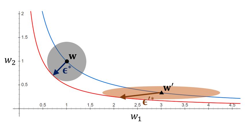
ASAM: Adaptive Sharpness-Aware Minimization for Scale-Invariant Learning of Deep Neural Networks

mizes the corresponding generalization bound using adap-          radius ρ for p ≥ 1. Here, sharpness of the loss function L is
tive sharpness to generalize on unseen data, avoiding the         defined as
scale-dependency issue SAM suffers from.
                                                                                    max LS (w + ) − LS (w).                (2)
The main contributions of this paper are summarized as                           kk2 ≤ρ

follows:                                                          Because of the monotonicity of h in Equation 1, it can
                                                                  be substituted by `2 weight decaying regularizer, so the
   • We introduce adaptive sharpness of loss surface which        sharpness-aware minimization problem can be defined as
     is invariant to parameter re-scaling. In terms of rank       the following minimax optimization
     statistics, adaptive sharpness shows stronger correla-
     tion with generalization than sharpness does, which                                                   λ
                                                                               min max LS (w + ) +          kwk22
     means that adaptive sharpness is more effective mea-                       w kkp ≤ρ                  2
     sure of generalization gap.                                  where λ is a weight decay coefficient.
   • We propose a new learning algorithm using adaptive           SAM solves the minimax problem by iteratively applying
     sharpness which helps alleviate the side-effect in train-    the following two-step procedure for t = 0, 1, 2, . . . as
     ing procedure caused by scale-dependency by adjusting
                                                                                   ∇LS (wt )
                                                                       (
     their maximization region with respect to weight scale.               t = ρ
                                                                                  k∇LS (wt )k2                               (3)
   • We empirically show its consistent improvement of                     wt+1 = wt − αt (∇LS (wt + t ) + λwt )
     generalization performance on image classification and
     machine translation tasks using various neural network       where αt is an appropriately scheduled learning rate. This
     architectures.                                               procedure can be obtained by a first order approximation of
                                                                  LS and dual norm formulation as
The rest of this paper is organized as follows. Section 2                  t = arg max LS (wt + )
briefly describes previous sharpness-based learning algo-                         kkp ≤ρ

rithm. In Section 3, we introduce adaptive sharpness which                    ≈ arg max > ∇LS (wt )
is a scale-invariant measure of generalization gap after scale-                   kkp ≤ρ
dependent property of sharpness is explained. In Section 4,                                         |∇LS (wt )|q−1
ASAM algorithm is introduced in detail using the defini-                      = ρ sign(∇LS (wt ))
                                                                                                    k∇LS (wt )kqq−1
tion of adaptive sharpness. In Section 5, we evaluate the
generalization performance of ASAM for various models             and
and datasets. We provide the conclusion and future work in                                            λ
Section 6.                                                         wt+1 = arg min LS (w + t ) +        kwk22
                                                                                w                     2
                                                                                                                      λ
2. Preliminary                                                            ≈ arg min (w − wt )> ∇LS (wt + t ) +         kwk22
                                                                                w                                     2
Let us consider a model f : X → Y parametrized by a                       ≈ wt − αt (∇LS (wt + t ) + λwt )
weight vector w and a loss function l : Y × Y → R+ .
                                                                  where 1/p + 1/q = 1 and | · | denotes element-wise abso-
Given a sample S = {(x1 , y1 ), . . . , (xn , yn )} drawn from
                                                                  lute value function, and sign(·) also denotes element-wise
data distribution D with P
                         i.i.d condition, the training loss can
                            n                                     signum function. It is experimentally confirmed that the
be defined as LS (w) = i=1 l(yi , f (xi ; w))/n. Then, the
                                                                  above two-step procedure produces the best performance
generalization gap between the expected loss LD (w) =
                                                                  when p = 2, which results in Equation 3.
E(x,y)∼D [l(y, f (x; w))] and the training loss LS (w) rep-
resents the ability of the model to generalize on unseen          As can be seen from Equation 3, SAM estimates the point
data.                                                             wt + t at which the loss is approximately maximized
                                                                  around wt in a rigid region with a fixed radius by perform-
Sharpness-Aware Minimization (SAM) (Foret et al., 2021)
                                                                  ing gradient ascent, and performs gradient descent at wt
aims to minimize the following PAC-Bayesian generaliza-
                                                                  using the gradient at the maximum point wt + t .
tion error upper bound

                                                kwk22
                                                                 3. Adaptive Sharpness: Scale-Invariant
       LD (w) ≤ max LS (w + ) + h                          (1)      Measure of Generalization Gap
                   kkp ≤ρ                       ρ2
for some strictly increasing function h. The domain of max        In Foret et al. (2021), it is experimentally confirmed that
operator, called maximization region, is an `p ball with          the sharpness defined in Equation 2 is strongly correlated
ASAM: Adaptive Sharpness-Aware Minimization for Scale-Invariant Learning of Deep Neural Networks
with the generalization gap. Also they show that SAM
helps to find minima which show lower sharpness than other
learning strategies and contributes to effectively lowering
generalization error.
However, Dinh et al. (2017) show that sharpness defined
in the rigid spherical region with a fixed radius can have
a weak correlation with the generalization gap due to non-
identifiability of rectifier neural networks, whose parameters
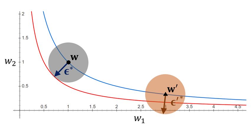
can be freely re-scaled without affecting its output. (a) kk2 ≤ ρ and k0 k2 ≤ ρ (Foret et al., 2021)
If we assume that A is a scaling operator on the weight
space that does not change the loss function, as shown in
Figure 1(a), the interval of the loss contours around Aw
becomes narrower than that around w but the size of the
region remains the same, i.e.,
max LS (w + ) 6= max LS (Aw + ).
kk2 ≤ρ kk2 ≤ρ
Thus, neural networks with w and Aw can have arbitrarily
different values of sharpness defined in Equation 2, although −1
(b) kTw −1 0
k∞ ≤ ρ and kTw 0 k∞ ≤ ρ (Keskar et al.,
they have the same generalization gaps. This property of 2017)
sharpness is a main cause of weak correlation between
generalization gap and sharpness and we call this scale-
dependency in this paper.
To solve the scale-dependency of sharpness, we introduce
the concept of adaptive sharpness. Prior to explaining adap-
tive sharpness, we first define normalization operator. The
normalization operator that cancels out the effect of A can
be defined as follows.
Definition 1 (Normalization operator). Let {Tw , w ∈ Rk }
−1 −1 0
be a family of invertible linear operators on Rk . Given (c) kTw k2 ≤ ρ and kTw 0 k2 ≤ ρ (In this paper)
−1 −1
a weight w, if TAw A = Tw for any invertible scaling
k
operator A on R which does not change the loss function, Figure 1. Loss contours and three types of maximization regions:
−1 (a) sphere, (b) cuboid and (c) ellipsoid. w = (1, 1) and w0 =
we say Tw is a normalization operator of w.
(3, 1/3) are parameter points before and after multiplying a scaling
Using the normalization operator, we define adaptive sharp- operator A = diag(3, 1/3) and are expressed as dots and triangles,
ness as follows. respectively. The blue contour line has the same loss at w, and the
−1 red contour line has a loss equal to the maximum value of the loss
Definition 2 (Adaptive sharpness). If Tw is the normaliza-
tion operator of w in Definition 1, adaptive sharpness of w in each type of region centered on w. ∗ and 0∗ are the and 0
which maximize the loss perturbed from w and w0 , respectively.
is defined by
max LS (w + ) − LS (w) (4) −1 −1
−1
kTw kp ≤ρ where Tw and TAw are the normalization operators of w
where 1 ≤ p ≤ ∞. and Aw in Definition 1, respectively.
Adaptive sharpness in Equation 4 has the following proper- Proof. From the assumption, it suffices to show that the
ties. first terms of both sides are equal. By the definition of the
−1 −1
Theorem 1. For any invertible scaling operator A which normalization operator, we have TAw A = Tw . Therefore,
does not change the loss function, values of adaptive sharp-
max LS (Aw + ) = max LS (w + A−1 )
ness at w and Aw are the same as −1
kTAw kp ≤ρ −1
kTAw kp ≤ρ
−1
max LS (w + ) − LS (w) = −1
max LS (w + 0 )
kTw kp ≤ρ kTAw A0 kp ≤ρ
= −1
max LS (Aw + ) − LS (Aw) = max
−1 0
LS (w + 0 )
kTAw kp ≤ρ kTw kp ≤ρASAM: Adaptive Sharpness-Aware Minimization for Scale-Invariant Learning of Deep Neural Networks
where 0 = A−1 . 0.30 0.30
Generalization gap
Generalization gap
By Theorem 1, adaptive sharpness defined in Equation 4 is 0.25 0.25
scale-invariant as with training loss and generalization loss.
0.20 0.20
This property makes the correlation of adaptive sharpness
with the generalization gap stronger than that of sharpness 0.15 0.15
in Equation 2.
0.0000 0.0001 0.0 0.5 1.0
Figure 1(b) and 1(c) show how a re-scaled weight vector Sharpness Adaptive Sharpness
can have the same adaptive sharpness value as that of the
original weight vector. It can be observed that the boundary (a) Sharpness (p = 2), (b) Adaptive sharpness (p = 2),
τ = 0.174. τ = 0.636.
line of each region centered on w0 is in contact with the red
line. This implies that the maximum loss within each region 0.30
−1 0
centered on w0 is maintained when kTw 0 kp ≤ ρ is used
Generalization gap
Generalization gap
0.25
for the maximization region. Thus, in this example, it can 0.25
be seen that adaptive sharpness in 1(b) and 1(c) has scale-
0.20 0.20
invariant property in contrast to sharpness of the spherical
region shown in Figure 1(a). 0.15 0.15
The question that can be asked here is what kind of operators
0 5 10 0 2 4
Tw can be considered as normalization operators which Sharpness Adaptive Sharpness
−1 −1
satisfy TAw A = Tw for any A which does not change the
loss function. One of the conditions for the scaling operator (c) Sharpness (p = ∞), (d) Adaptive sharpness
τ = 0.257. (p = ∞), τ = 0.616.
A that does not change the loss function is that it should
be node-wise scaling, which corresponds to row-wise or
Figure 2. Scatter plots which show correlation of sharpness and
column-wise scaling in fully-connected layers and channel-
adaptive sharpness with respect to generalization gap and their
wise scaling in convolutional layers. The effect of such rank correlation coefficients τ .
node-wise scaling can be canceled using the inverses of the
following operators:
To confirm that adaptive sharpness actually has a stronger
• element-wise
correlation with generalization gap than sharpness, we com-
pare rank statistics which demonstrate the change of adap-
Tw = diag(|w1 |, . . . , |wk |)
tive sharpness and sharpness with respect to generalization
where gap. For correlation analysis, we use 4 hyper-parameters:
w = [w1 , w2 , . . . , wk ], mini-batch size, initial learning rate, weight decay coeffi-
cient and dropout rate. As can be seen in Table 1, Kendall
• filter-wise rank correlation coefficient (Kendall, 1938) of adaptive
sharpness is greater than that of sharpness regardless of
Tw = diag(concat(kf1 k2 1n(f1 ) , . . . , kfm k2 1n(fm ) , the value of p. Furthermore, we compare granulated coef-
ficients (Jiang et al., 2019) with respect to different hyper-
|w1 |, . . . , |wq |)) (5)
parameters to measure the effect of each hyper-parameter
where separately. In Table 1, the coefficients of adaptive sharp-
ness are higher in most hyper-parameters and the average as
w = concat(f1 , f2 , . . . , fm , w1 , w2 , . . . , wq ). well. Scatter plots illustrated in Figure 2 also show stronger
correlation of adaptive sharpness. The difference in correla-
tion behaviors of adaptive sharpness and sharpness provides
Here, fi is the i-th flattened weight vector of a convolution
an evidence that scale-invariant property helps strengthen
filter and wj is the j-th weight parameter which is not in-
the correlation with generalization gap. The experimental
cluded in any filters. And m is the number of filters and
details are described in Appendix B.
q is the number of other weight parameters in the model.
If there is no convolutional layer in a model (i.e., m = 0), Although there are various normalization methods other
then q = k and both normalization operators are identical than the normalization operators introduced above, this pa-
to each other. Note that we use Tw + ηIk rather than Tw for per covers only element-wise and filter-wise normalization
sufficiently small η > 0 for stability. η is a hyper-parameter operators. Node-wise normalization can also be viewed as
controlling trade-off between adaptivity and stability. a normalization operator. Tsuzuku et al. (2020) suggestASAM: Adaptive Sharpness-Aware Minimization for Scale-Invariant Learning of Deep Neural Networks
Also, sharpness suggested in Keskar et al. (2017) can be
Table 1. Rank statistics for sharpness and adaptive sharpness.
regarded as a special case of adaptive sharpness which uses
p=2 p=∞ p = ∞ and the element-wise normalization operator. Jiang
adaptive adaptive et al. (2019) confirm experimentally that the adaptive sharp-
sharpness sharpness ness suggested in Keskar et al. (2017) shows a higher cor-
sharpness sharpness
τ (rank corr.) 0.174 0.636 0.257 0.616 relation with the generalization gap than sharpness which
mini-batch size 0.667 0.696 0.777 0.817 does not use element-wise normalization operator. This ex-
learning rate 0.563 0.577 0.797 0.806 perimental result implies that Theorem 1 is also practically
weight decay −0.297 0.534 −0.469 0.656 validated.
dropout rate 0.102 −0.092 0.161 0.225
Ψ (avg.) 0.259 0.429 0.316 0.626 Therefore, it seems that sharpness with p = ∞ suggested
by Keskar et al. (2017) also can be used directly for learn-
ing as it is, but a problem arises in terms of generalization
performance in learning. Foret et al. (2021) confirm experi-
node-wise normalization method for obtaining normalized mentally that the generalization performance with sharpness
flatness. However, the method requires that the parameter defined in square region kk∞ ≤ ρ result is worse than
should be at a critical point. Also, in the case of node-wise when SAM is performed with sharpness defined in spherical
normalization using unit-invariant SVD (Uhlmann, 2018), region kk2 ≤ ρ.
there is a concern that the speed of the optimizer can be
degraded due to the significant additional cost for scale- We conduct performance comparison tests for p = 2 and
direction decomposition of weight tensors. Therefore the p = ∞, and experimentally reveal that p = 2 is more suit-
node-wise normalization is not covered in this paper. In able for learning as in Foret et al. (2021). The experimental
the case of layer-wise normalization using spectral norm or results are shown in Section 5.
Frobenius norm of weight matrices (Neyshabur et al., 2017),
−1 −1
the condition TAw A = Tw is not satisfied. Therefore, it 4. Adaptive Sharpness-Aware Minimization
cannot be used for adaptive sharpness so we do not cover it
in this paper. In the previous section, we introduce a scale-invariant mea-
sure called adaptive sharpness to overcome the limitation of
Meanwhile, even though all weight parameters including bi- sharpness. As in sharpness, we can obtain a generalization
ases can have scale-dependency, there remains more to con- bound using adaptive sharpness, which is presented in the
sider when applying normalization to the biases. In terms following theorem.
of bias parameters of rectifier neural networks, there also −1
Theorem 2. Let Tw be the normalization operator on Rk .
exists translation-dependency in sharpness, which weakens
If LD (w) ≤ Ei ∼N (0,σ2 ) [LD (w+)] for some σ > 0, then
the correlation with the generalization gap as well. Us-
with probability 1 − δ,
ing the similar arguments as in the proof of Theorem 1, it
can be derived that diagonal elements of Tw correspond-
kwk22
ing to biases must be replaced by constants to guarantee LD (w) ≤ max LS (w + ) + h (6)
kTw−1
k2 ≤ρ η 2 ρ2
translation-invariance, which induces adaptive sharpness
that corresponds to the case of not applying bias normaliza-
where h : R+√→ R+ isp
a strictly increasing function, n =
tion. We compare the generalization performance based on
|S| and ρ = kσ(1 + log n/k)/η.
adaptive sharpness with and without bias normalization, in
Section 5. Note that Theorem 2 still holds for p > 2 due to the mono-
There are several previous works which are closely related tonicity of p-norm, i.e., if 0 < r < p, kxkp ≤ kxkr for
to adaptive sharpness. Li et al. (2018), which suggest a any x ∈ Rn . If Tw is an identity operator, Equation 6 is
methodology for visualizing loss landscape, is related to reduced equivalently to Equation 1. The proof of Equation 6
adaptive sharpness. In that study, filter-wise normalization is described in detail in Appendix A.1.
which is equivalent to the definition in Equation 5 is used The right hand side of Equation 6, i.e., generalization bound,
to remove scale-dependency from loss landscape and make can be expressed using adaptive sharpness as
comparisons between loss functions meaningful. In spite
of their empirical success, Li et al. (2018) do not provide a
!
kwk22
theoretical evidence for explaining how filter-wise scaling max LS (w + ) − LS (w) + LS (w) + h .
−1
kTw kp ≤ρ η 2 ρ2
contributes the scale-invariance and correlation with gen-
eralization. In this paper, we clarify how the filter-wise
normalization relates to generalization by proving the scale- Since h kwk22 /η 2 ρ2 is a strictly increasing function with
invariant property of adaptive sharpness in Theorem 1. respect to kwk22 , it can be substituted with `2 weight decay-ASAM: Adaptive Sharpness-Aware Minimization for Scale-Invariant Learning of Deep Neural Networks
Algorithm 1 ASAM algorithm (p = 2) 0.25 0.
04
Input: Loss function l, training dataset S := 0.
0.20 02
∪ni=1 {(xi , yi )}, mini-batch size b, radius of maximiza- 0.0
3
tion region ρ, weight decay coefficient λ, scheduled learn- 0.0
ing rate α, initial weight w0 . 0.15 1
w2
Output: Trained weight w
0.10
Initialize weight w := w0 0.01
while not converged do 0.02
0.05 SAM
Sample a mini-batch B of size b from S ASAM 0.03
T 2 ∇LB (w)
:= ρ w 0.00
kTw ∇LB (w)k2 0.0 0.1 0.2 0.3 0.4
†
w := w − α (∇LB (w + ) + λw) w1
end while
return w Figure 3. Trajectories of SAM and ASAM.
ing regularizer. Therefore, we can define adaptive sharpness-
aware minimization problem as
5. Experimental Results
λ
min max LS (w + ) + kwk22 . (7) In this section, we evaluate the performance of ASAM. We
w kT −1 kp ≤ρ
w
2
first show how SAM and ASAM operate differently in a toy
To solve the minimax problem in Equation 7, it is neces- example. We then compare the generalization performance
sary to find optimal first. Analogous to SAM, we can of ASAM with other learning algorithms for various model
approximate the optimal to maximize LS (w + ) using a architectures and various datasets: CIFAR-10, CIFAR-100
first-order approximation as (Krizhevsky et al., 2009), ImageNet (Deng et al., 2009) and
IWSLT’14 DE-EN (Cettolo et al., 2014). Finally, we show
˜t = arg max LS (wt + Twt ˜) how robust to label noise ASAM is.
k˜
kp ≤ρ
≈ arg max ˜> Twt ∇LS (wt ) 5.1. Toy Example
k˜
kp ≤ρ
|Twt ∇LS (wt )|q−1 As mentioned in Section 4, sharpness varies by parameter
= ρ sign(∇LS (wt )) re-scaling even if its loss function remains the same, while
kTwt ∇LS (wt )kq−1
q
adaptive sharpness does not. To elaborate this, we con-
−1 sider a simple loss function L(w) = |w1 ReLU(w2 ) − 0.04|
where ˜ = Tw . Then, the two-step procedure for adaptive
sharpness-aware minimization (ASAM) is expressed as where w = (w1 , w2 ) ∈ R2 . Figure 3 presents the trajecto-
ries of SAM and ASAM with two different initial weights
= ρT sign(∇L (w )) |Twt ∇LS (wt )|q−1
t wt S t
w0 = (0.2, 0.05) and w0 = (0.3, 0.033). The red line rep-
kTwt ∇LS (wt )kq−1
q resents the set of minimizers of the loss function L, i.e.,
wt+1 = wt − αt (∇LS (wt + t ) + λwt )
{(w1 , w2 ); w1 w2 = 0.04, w2 > 0}. As seen in Figure 1(a),
for t = 0, 1, 2, · · · . Especially, if p = 2, sharpness is maximized when w1 = w2 within the same
loss contour line, and therefore SAM tries to converge to
2
Tw t
∇LS (wt ) (0.2, 0.2). Here, we use ρ = 0.05 as in Foret et al. (2021).
t = ρ On the other hand, adaptive sharpness remains the same
kTwt ∇LS (wt )k2
along the same contour line which implies that ASAM con-
and if p = ∞, verges to the point in the red line near the initial point as
t = ρTwt sign(∇LS (wt )). can be seen in Figure 3.
Since SAM uses a fixed radius in a spherical region for
In this study, experiments are conducted on ASAM in cases minimizing sharpness, it may cause undesirable results de-
of p = ∞ and p = 2. The ASAM algorithm with p = 2 pending on the loss surface and the current weight. If
is described in detail on Algorithm 1. Note that the SGD w0 = (0.3, 0.033), while SAM even fails to converge to the
(Nesterov, 1983) update marked with † in Algorithm 1 can valley with ρ =√0.05, ASAM converges no matter which w0
be combined with momentum or be replaced by update of is used if ρ < 2. In other words, appropriate ρ for SAM
another optimization scheme such as Adam (Kingma & Ba, is dependent on the scales of w on the training trajectory,
2015). whereas ρ of ASAM is not.ASAM: Adaptive Sharpness-Aware Minimization for Scale-Invariant Learning of Deep Neural Networks
Table 2. Maximum test accuracies for SGD, SAM and ASAM on
CIFAR-10 dataset.
Model SGD SAM ASAM
97.5 DenseNet-121 91.00±0.13 92.00±0.17 93.33±0.04
ResNet-20 93.18±0.21 93.56±0.15 93.82±0.17
ResNet-56 94.58±0.20 95.18±0.15 95.42±0.16
Test Accuracy (%)
97.0 VGG19-BN∗ 93.87±0.09 94.60 95.07±0.05
ResNeXt29-32x4d 95.84±0.24 96.34±0.30 96.80±0.06
WRN-28-2 95.13±0.16 95.74±0.08 95.94±0.05
96.5 WRN-28-10 96.34±0.12 96.98±0.04 97.28±0.07
PyramidNet-272† 98.44±0.08 98.55±0.05 98.68±0.08
p = ∞, element-wise *
96.0 p = 2, element-wise
Some runs completely failed, thus giving 10% of accuracy (suc-
cess rate: SGD: 3/5, SAM 1/5, ASAM 3/5)
p = 2, element-wise (w/ BN) †
PyramidNet-272 architecture is tested 3 times for each learning
p = 2, filter-wise
algorithm.
10−5 10−4 10−3 10−2 10−1 100 101
ρ
Table 3. Maximum test accuracies for SGD, SAM and ASAM on
Figure 4. Test accuracy curves obtained from ASAM algorithm CIFAR-100 dataset.
using a range of ρ with different factors: element-wise normaliza- Model SGD SAM ASAM
tion with p = ∞, element-wise normalization with p = 2 with
DenseNet-121 68.70±0.31 69.84±0.12 70.60±0.20
and without bias normalization (BN) and filter-wise normalization
ResNet-20 69.76±0.44 71.06±0.31 71.40±0.30
with p = 2. ResNet-56 73.12±0.19 75.16±0.05 75.86±0.22
VGG19-BN∗ 71.80±1.35 73.52±1.74 75.80±0.27
ResNeXt29-32x4d 79.76±0.23 81.48±0.17 82.30±0.11
WRN-28-2 75.28±0.17 77.25±0.35 77.54±0.14
5.2. Image Classification: CIFAR-10/100 and ImageNet WRN-28-10 81.56±0.13 83.42±0.04 83.68±0.12
PyramidNet-272† 88.91±0.12 89.36±0.20 89.90±0.13
To confirm the effectiveness of ASAM, we conduct compar-
*
ison experiments with SAM using CIFAR-10 and CIFAR- Some runs completely failed, thus giving 10% of accuracy (suc-
cess rate: SGD: 5/5, SAM 4/5, ASAM 4/5)
100 datasets. We use the same data split as the original paper †
PyramidNet-272 architecture is tested 3 times for each learning
(Krizhevsky et al., 2009). The hyper-parameters used in this algorithm.
test is described in Table 3. Before the comparison tests
with SAM, there are three factors to be chosen in ASAM
algorithm:
operator and p = 2, and not to employ bias normalization
in the remaining tests.
• normalization schemes: element-wise vs. filter-wise
As ASAM has a hyper-parameter ρ to be tuned, we first
• p-norm: p = ∞ vs. p = 2 conduct a grid search over {0.00005, 0.0001, 0.0002, . . . ,
0.5, 1.0, 2.0} for finding appropriate values of ρ. We use
• bias normalization: with vs. without ρ = 0.5 for CIFAR-10 and ρ = 1.0 for CIFAR-100, be-
cause it gives moderately good performance across various
First, we perform the comparison test for filter-wise and models. We set ρ for SAM as 0.05 for CIFAR-10 and 0.1
element-wise normalization using WideResNet-16-8 model for CIFAR-100 as in Foret et al. (2021). η for ASAM is set
(Zagoruyko & Komodakis, 2016) and illustrate the results to 0.01. We set mini-batch size to 128, and m-sharpness
in Figure 4. As can be seen, both test accuracies are compa- suggested by Foret et al. (2021) is not employed. The num-
rable across ρ, and element-wise normalization provides a ber of epochs is set to 200 for SAM and ASAM and 400
slightly better accuracy at ρ = 1.0. for SGD. Momentum and weight decay coefficient are set
to 0.9 and 0.0005, respectively. Cosine learning rate decay
Similarly, Figure 4 shows how much test accuracy varies
(Loshchilov & Hutter, 2016) is adopted with an initial learn-
with the maximization region for adaptive sharpness. It can
ing rate 0.1. Also, random resize, padding by four pixels,
be seen that p = 2 shows better test accuracies than p =
normalization and random horizontal flip are applied for
∞, which is consistent with Foret et al. (2021). We could
data augmentation and label smoothing (Müller et al., 2019)
also observe that ASAM with bias normalization does not
is adopted with its factor of 0.1.
contribute to the improvement of test accuracy in Figure 4.
Therefore, we decide to use element-wise normalization Using the hyper-parameters, we compare the best test ac-ASAM: Adaptive Sharpness-Aware Minimization for Scale-Invariant Learning of Deep Neural Networks
curacies obtained by SGD, SAM and ASAM for various β2 for Adam are set to 0.0005, 0.9 and 0.98, respectively.
rectifier neural network models: VGG (Simonyan & Zis- Dropout rate and weight decay coefficient are set to 0.3 and
serman, 2015), ResNet (He et al., 2016), DenseNet (Huang 0.0001, respectively. Label smoothing is adopted with its
et al., 2017), WideResNet (Zagoruyko & Komodakis, 2016), factor 0.1. We choose ρ = 0.1 for SAM and ρ = 0.2 for
and ResNeXt (Xie et al., 2017). ASAM as a result of a grid search over {0.005, 0.01, 0.02,
. . . , 0.5, 1.0, 2.0} using validation dataset. The results of
For PyramidNet-272 (Han et al., 2017), we additionally
the experiments are obtained from 3 independent runs.
apply some latest techniques: AutoAugment (Cubuk et al.,
2019), CutMix (Yun et al., 2019) and ShakeDrop (Yamada As can be seen in Table 5, we could observe improve-
et al., 2019). We employ the m-sharpness strategy with ment even on IWSLT’14 in BLEU score when using
m = 32. Initial learning rate and mini-batch size are set to Adam+ASAM instead of Adam or Adam+SAM.
0.05 and 256, respectively. The number of epochs is set to
900 for SAM and ASAM and 1800 for SGD. We choose ρ
Table 5. BLEU scores for Adam, Adam+SAM and Adam+ASAM
for SAM as 0.05, as in Foret et al. (2021), and ρ for ASAM on IWSLT’14 DE-EN dataset using Transformer.
as 1.0 for both CIFAR-10 and CIFAR-100. Every entry
in the tables represents mean and standard deviation of 5 BLEU score Adam Adam+SAM Adam+ASAM
independent runs. In both CIFAR-10 and CIFAR-100 cases, Validation 35.34±ASAM: Adaptive Sharpness-Aware Minimization for Scale-Invariant Learning of Deep Neural Networks
property, which ASAM shares, contributes in improvement ference on Machine Learning, pp. 1019–1028. PMLR,
of generalization performance. The superior performance 2017.
of ASAM is notable from the comparison tests conducted
against SAM, which is currently state-of-the-art learning Foret, P., Kleiner, A., Mobahi, H., and Neyshabur, B.
algorithm in many image classification benchmarks. In Sharpness-aware minimization for efficiently improving
addition to the contribution as a learning algorithm, adap- generalization. In International Conference on Learning
tive sharpness can serve as a generalization measure with Representations, 2021.
stronger correlation with generalization gap benefiting from
Han, D., Kim, J., and Kim, J. Deep pyramidal residual
their scale-invariant property. Therefore adaptive sharp-
networks. In Proceedings of the IEEE conference on
ness has a potential to be a metric for assessment of neural
computer vision and pattern recognition, pp. 5927–5935,
networks. We have also suggested the condition of nor-
2017.
malization operator for adaptive sharpness but we did not
cover all the normalization schemes which satisfy the con- He, K., Zhang, X., Ren, S., and Sun, J. Deep residual learn-
dition. So this area could be further investigated for better ing for image recognition. In Proceedings of the IEEE
generalization performance in future works. conference on computer vision and pattern recognition,
pp. 770–778, 2016.
7. Acknowledgements
Hochreiter, S. and Schmidhuber, J. Flat minima. Neural
We would like to thank Kangwook Lee, Jaedeok Kim and computation, 9(1):1–42, 1997.
Yonghyun Ryu for supports on our machine translation ex-
periments. We also thank our other colleagues at Samsung Hochreiter, S., Schmidhuber, J., et al. Simplifying neural
Research - Joohyung Lee, Chiyoun Park and Hyun-Joo Jung nets by discovering flat minima. Advances in neural
- for their insightful discussions and feedback. information processing systems, pp. 529–536, 1995.
Huang, G., Liu, Z., Van Der Maaten, L., and Weinberger,
References K. Q. Densely connected convolutional networks. In
Cettolo, M., Niehues, J., Stüker, S., Bentivogli, L., and Fed- Proceedings of the IEEE conference on computer vision
erico, M. Report on the 11th IWSLT evaluation campaign, and pattern recognition, pp. 4700–4708, 2017.
IWSLT 2014. In Proceedings of the International Work-
Jiang, L., Huang, D., Liu, M., and Yang, W. Beyond syn-
shop on Spoken Language Translation, Hanoi, Vietnam,
thetic noise: Deep learning on controlled noisy labels.
volume 57, 2014.
In International Conference on Machine Learning, pp.
Chatterji, N., Neyshabur, B., and Sedghi, H. The intriguing 4804–4815. PMLR, 2020.
role of module criticality in the generalization of deep
networks. In International Conference on Learning Rep- Jiang, Y., Neyshabur, B., Mobahi, H., Krishnan, D., and
resentations, 2019. Bengio, S. Fantastic generalization measures and where
to find them. In International Conference on Learning
Chaudhari, P., Choromanska, A., Soatto, S., LeCun, Y., Bal- Representations, 2019.
dassi, C., Borgs, C., Chayes, J., Sagun, L., and Zecchina,
R. Entropy-sgd: Biasing gradient descent into wide val- Karakida, R., Akaho, S., and Amari, S.-i. The normalization
leys. Journal of Statistical Mechanics: Theory and Ex- method for alleviating pathological sharpness in wide
periment, 2019(12):124018, 2019. neural networks. In Advances in Neural Information
Processing Systems, volume 32. Curran Associates, Inc.,
Cubuk, E. D., Zoph, B., Mane, D., Vasudevan, V., and Le, 2019.
Q. V. Autoaugment: Learning augmentation strategies
from data. In Proceedings of the IEEE/CVF Conference Kendall, M. G. A new measure of rank correlation.
on Computer Vision and Pattern Recognition, pp. 113– Biometrika, 30(1/2):81–93, 1938.
123, 2019.
Keskar, N. S., Nocedal, J., Tang, P. T. P., Mudigere, D.,
Deng, J., Dong, W., Socher, R., Li, L.-J., Li, K., and Fei-Fei, and Smelyanskiy, M. On large-batch training for deep
L. ImageNet: A large-scale hierarchical image database. learning: Generalization gap and sharp minima. In 5th
In 2009 IEEE conference on computer vision and pattern International Conference on Learning Representations,
recognition, pp. 248–255. IEEE, 2009. ICLR 2017, 2017.
Dinh, L., Pascanu, R., Bengio, S., and Bengio, Y. Sharp min- Kingma, D. P. and Ba, J. Adam: A method for stochastic
ima can generalize for deep nets. In International Con- optimization. In ICLR (Poster), 2015.ASAM: Adaptive Sharpness-Aware Minimization for Scale-Invariant Learning of Deep Neural Networks
Krizhevsky, A., Nair, V., and Hinton, G. CIFAR-10 and Sun, X., Zhang, Z., Ren, X., Luo, R., and Li, L. Exploring
CIFAR-100 datasets. 2009. URL https://www.cs. the vulnerability of deep neural networks: A study of
toronto.edu/~kriz/cifar.html. parameter corruption. CoRR, abs/2006.05620, 2020.
Laurent, B. and Massart, P. Adaptive estimation of a Tsuzuku, Y., Sato, I., and Sugiyama, M. Normalized flat
quadratic functional by model selection. Annals of Statis- minima: Exploring scale invariant definition of flat min-
tics, pp. 1302–1338, 2000. ima for neural networks using PAC-Bayesian analysis.
In International Conference on Machine Learning, pp.
Li, H., Xu, Z., Taylor, G., Studer, C., and Goldstein, T. 9636–9647. PMLR, 2020.
Visualizing the loss landscape of neural nets. In NIPS’18:
Proceedings of the 32nd International Conference on Uhlmann, J. A generalized matrix inverse that is consistent
Neural Information Processing Systems, pp. 6391–6401. with respect to diagonal transformations. SIAM Jour-
Curran Associates Inc., 2018. nal on Matrix Analysis and Applications, 39(2):781–800,
2018.
Liang, T., Poggio, T., Rakhlin, A., and Stokes, J. Fisher-rao
metric, geometry, and complexity of neural networks. In Vaswani, A., Shazeer, N., Parmar, N., Uszkoreit, J., Jones,
The 22nd International Conference on Artificial Intelli- L., Gomez, A. N., Kaiser, L., and Polosukhin, I. Attention
gence and Statistics, pp. 888–896. PMLR, 2019. is all you need. In NIPS, 2017.
Loshchilov, I. and Hutter, F. Sgdr: Stochastic gra- Xie, S., Girshick, R., Dollár, P., Tu, Z., and He, K. Aggre-
dient descent with warm restarts. arXiv preprint gated residual transformations for deep neural networks.
arXiv:1608.03983, 2016. In Proceedings of the IEEE conference on computer vi-
sion and pattern recognition, pp. 1492–1500, 2017.
McAllester, D. A. PAC-Bayesian model averaging. In
Proceedings of the twelfth annual conference on Compu- Yamada, Y., Iwamura, M., Akiba, T., and Kise, K. Shake-
tational learning theory, pp. 164–170, 1999. drop regularization for deep residual learning. IEEE
Access, 7:186126–186136, 2019.
Mobahi, H. Training recurrent neural networks by diffusion.
arXiv preprint arXiv:1601.04114, 2016. Yi, M., Meng, Q., Chen, W., Ma, Z.-m., and Liu, T.-Y.
Positively scale-invariant flatness of relu neural networks.
Müller, R., Kornblith, S., and Hinton, G. E. When does arXiv preprint arXiv:1903.02237, 2019.
label smoothing help? In Wallach, H., Larochelle, H.,
Beygelzimer, A., d'Alché-Buc, F., Fox, E., and Garnett, Yue, X., Nouiehed, M., and Kontar, R. A. Salr: Sharpness-
R. (eds.), Advances in Neural Information Processing aware learning rates for improved generalization. arXiv
Systems, volume 32. Curran Associates, Inc., 2019. preprint arXiv:2011.05348, 2020.
Nesterov, Y. E. A method for solving the convex program- Yun, S., Han, D., Oh, S. J., Chun, S., Choe, J., and Yoo,
ming problem with convergence rate O(1/k 2 ). In Dokl. Y. CutMix: Regularization strategy to train strong clas-
akad. nauk Sssr, volume 269, pp. 543–547, 1983. sifiers with localizable features. In Proceedings of the
IEEE/CVF International Conference on Computer Vision,
Neyshabur, B., Bhojanapalli, S., Mcallester, D., and Srebro, pp. 6023–6032, 2019.
N. Exploring generalization in deep learning. In Guyon,
I., Luxburg, U. V., Bengio, S., Wallach, H., Fergus, R., Zagoruyko, S. and Komodakis, N. Wide residual networks.
Vishwanathan, S., and Garnett, R. (eds.), Advances in CoRR, abs/1605.07146, 2016.
Neural Information Processing Systems, volume 30. Cur-
ran Associates, Inc., 2017.
Rooyen, B. v., Menon, A. K., and Williamson, R. C. Learn-
ing with symmetric label noise: the importance of be-
ing unhinged. In Proceedings of the 28th International
Conference on Neural Information Processing Systems-
Volume 1, pp. 10–18, 2015.
Simonyan, K. and Zisserman, A. Very deep convolutional
networks for large-scale image recognition. In 3rd Inter-
national Conference on Learning Representations, ICLR
2015, San Diego, CA, USA, May 7-9, 2015, Conference
Track Proceedings, 2015.You can also read