Atlas of Urban Scaling Laws
←
→
Page content transcription
If your browser does not render page correctly, please read the page content below
Atlas of Urban Scaling Laws

                                                                                           Anna Carbone and Pietro Murialdo
                                                                                                 Politecnico di Torino Italy

                                                                                                     Alessandra Pieroni
                                                                                                 Agenzia per l’Italia Digitale
                                                                                                        Roma Italy

                                                                                                    Carina Toxqui-Quitl
                                                                                            Universidad Politécnica de Tulancingo
arXiv:2109.11050v1 [physics.soc-ph] 22 Sep 2021

                                                                                                      Hidalgo Mexico
                                                                                                 (Dated: September 24, 2021)

                                                                 Highly accurate estimates of the urban fractal dimension Df are obtained by implementing the
                                                              Detrended Moving Average algorithm (DMA) on WorldView2 satellite high-resolution multi-spectral
                                                              images covering the largest European cities. Higher fractal dimensions are systematically obtained
                                                              for urban sectors (centrally located areas) than for suburban and peripheral areas, with Df values
                                                              ranging from 1.65 to 1.90 respectively.The exponents βs and βi of the scaling law N β with N
                                                              the population size, respectively for socio-economic and infrastructural variables, are evaluated for
                                                              different urban and suburban sectors in terms of the fractal dimension Df .Results confirm the range
                                                              of empirical values reported in the literature. Urban scaling laws have been traditionally derived
                                                              as if cities were zero-dimensional objects with the relevant feature related to a single homogeneous
                                                              population value, thus neglecting the microscopic heterogeneity of the urban structure. Our findings
                                                              allow one to go beyond this limit. High sensitive and repeatable satellite records yield robust local
                                                              estimates of the Hurst and scaling exponents. Furthermore, the approach allows one to discriminate
                                                              among different scaling theories, shedding light on the open issue of scaling phenomena, reconciling
                                                              contradictory scientific perspectives and pave paths to the systematic adoption of the complex
                                                              system science approach to urban landscape analysis.

                                                                  I.   INTRODUCTION                               [6] and synergetics [7] have been proposed. Common to
                                                                                                                  these studies is the dependence of the interactions on the
                                                  The idea of quantifying socio-economic phenomena in             effective distance ` connecting any pair of sites, that for
                                                  terms of laws derived from statistical physics and com-         fractal media, can be expressed as ` ∝ λDf (Fig. 1). The
                                                  plex systems science continues to spread as highly ac-          exponent β is linked to the fractal (Hausdorff) dimension
                                                  curate time and space dependent data become avail-              Df of the background infrastructure, bridging the urban
                                                  able. Hence, early studies evidencing that diverse socio-       scaling and fractal geometry research areas together and
                                                  economic processes obey certain empirical laws can be           thus opening new directions to the quantitative analysis
                                                  supported by accurate data analysis and robust statis-          of socio-economic phenomena and urban complex sys-
                                                  tical modelling [1]. In this context, relevant urban fea-       tems.
                                                  tures Y have been linked to the population size N by
                                                  power-laws with exponents β > 1 typically observed for          Morphology and function of cities are prominent exam-
                                                  socio-economic features (e.g. patent production, gross          ples of fractals with the Haudorff dimension providing a
                                                  domestic product, crime, pollution), while physical in-         measure of the urban concentration across scales [8–10].
                                                  frastructure features (e.g. transportation, financial ser-      The estimation of fractal dimension in urban contexts
                                                  vices) tend to increase sublinearly with β < 1 and indi-        begins by analysing the spatial distribution of the build-
                                                  vidual needs (housing, water consumption) with β ≈ 1            up area, traditionally performed on cartographic images
                                                  (see e.g. [2] and references therein). Despite the diver-       with black pixels corresponding to build-up space and
                                                  sity of historical and geographical contexts, several ag-       resolution defined by the size of the pixels. While a uni-
                                                  gregated urban features are generally found to scale as         form distribution of buildings over the investigated area
                                                  power laws of population size, a behaviour whose micro-         would yield a fractal dimension almost equal to two, for
                                                  scopic origin is still under active debate. Diverse the-        a detached distribution of buildings, values lower than
                                                  ories, based on dissipative interactions [3], gravity [4],      two are expected. Urban infrastructures cannot be sim-
                                                  three-dimensional fractal buildings [5], self-organization      ply quantified by iteration of elementary constituents, as
                                                                                                                  it would be appropriate for deterministic fractals, and re-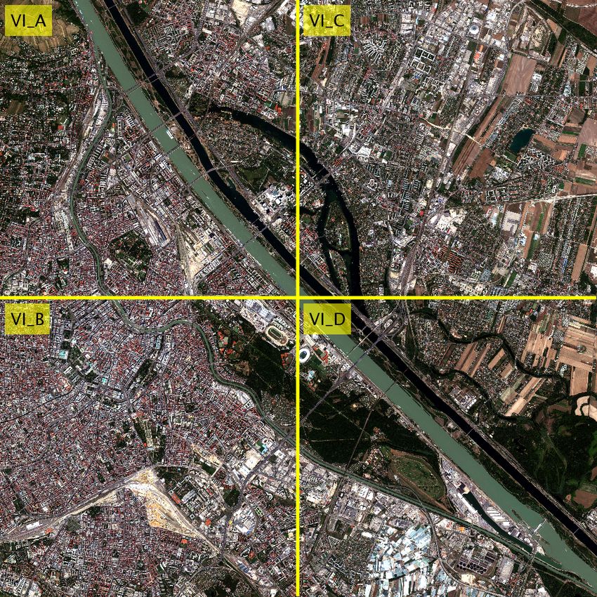
2

                                                                straints to their practical usability, requiring adequate
                                                                computational tools.

                                                                This work addresses some of the above challenges. We
                                                                provide statistically robust estimates of the Hurst expo-
                                                                nent H and fractal dimensions Df of urban and sub-
                                                                urban sectors by implementing the high-dimensional De-
                                                                trended Moving Average (DMA) [34] on 1.84m-resolution
                                                                Worldview-2 satellite images of several cities [35]. For
                                                                centrally located urban areas characterized by regular
                                                                building grid, fractal dimension values close to 1.9 are
                                                                found. Suburban and peripheral areas are characterised
                                                                by Df values close to 1.6. Next, the scaling exponents βs
                                                                and βi for the socio-economic and infrastructural quan-
                                                                tities are estimated. The dependence of βs and βi on
FIG. 1. Samples of individual paths between urban sites A
                                                                the fractal dimension Df is discussed on account of the
and B. Paths have characteristic length ` and include an area
                                                                expected behaviour and the empirical values reported in
A (cluster area). The length ` can be related to the aver-
age size (diameter) of the area λ = A1/d and to the fractal     previous studies. The proposed approach, by combining
dimension Df by the relationship ` ∝ λDf = ADf /d .             a very accurate computational method and high resolu-
                                                                tion repeatable satellite records data, yields statistically
                                                                robust estimates of the scaling properties of the urban
quire statistically based elaboration of data mapped on         sector structures. The outcomes are physically sound.
the coordinates i, j of the city grid. Methods as diverse       Overall, the approach could help to discriminate among
as box and radial counting [9–14], isarithm, triangular         limited insights and reconcile different controversial sci-
prism, and variogram [15–17] have been adopted to esti-         entific perspectives. The ultimate goal of this work is the
mate fractal features of urbanized areas. Different out-        achievement of a shared digital knowledge infrastructure
comes have been obtained even for the same city which           for urban landscape analysis of broad interest.
might be due to computing-method variations, disparities
in image size, map coverage and boundary, image resolu-         The manuscript is organized as follows. In Section II
tion, data accuracy, time period, box-size, and scale.          (Definitions and Methods) simple definition of the frac-
                                                                tal dimension and the DMA method are briefly recalled.
Despite extensive efforts and several successful applica-       In Section III (Data and Results) the Worldview-2 satel-
tions [18–23], many issues are still unsolved preventing        lite images are described and a few examples are shown
full acceptance of the urban scaling ideas [24–27]. Con-        and analysed (namely Turin, Wien, Zurich, Prague). The
cerns refer for example to the microscopic origin of the        Hurst exponent H and the fractal dimension Df are esti-
scaling behaviour and the analytical relationship linking       mated for different urban sectors, compared with previ-
the exponents β and Df , to the proper method and ac-           ously published results and validated against urban scal-
curacy of statistical fitting. The scaling exponent β and       ing models, in terms of the β vs. Df relationships, in Sec-
the fractal dimension Df heavily depend on the defini-          tion IV (Discussion). The main outcomes, potential im-
tions, methods and variables, chosen for their estima-          plications and directions for future work are summarised
tion, varying significantly among different works, thus         in Section V (Conclusion).
yielding different outcomes and irremediably defying the
intended universality. Heterogeneity and incompleteness
of the datasets represent a severe limitation to the accu-
racy and ultimately prevent comparability of the scaling                II.   DEFINITIONS AND METHODS
exponents and fractal dimensions across different cities.
High-resolution digitally collected data have the poten-        Self-similarity concepts and fractal geometry have been
tial to provide objective definitions and comparable es-        extensively adopted to describe real-world random struc-
timates across different regions. In particular, satel-         tures characterized by irregular fragmented shapes as
lite technologies yield regularly and uniformly recorded        well as other complex features that traditional ap-
data with well-defined features, conveniently exploited         proaches fail to grasp. Generally, scaling relations are
to gather information about infrastructural and socio-          obtained for self-similar textures in the form:
economic features [28–33]. However, the ever increas-
ing volume and complexity of data pose additional con-                                f (λ) ∝ λDf    ,                  (1)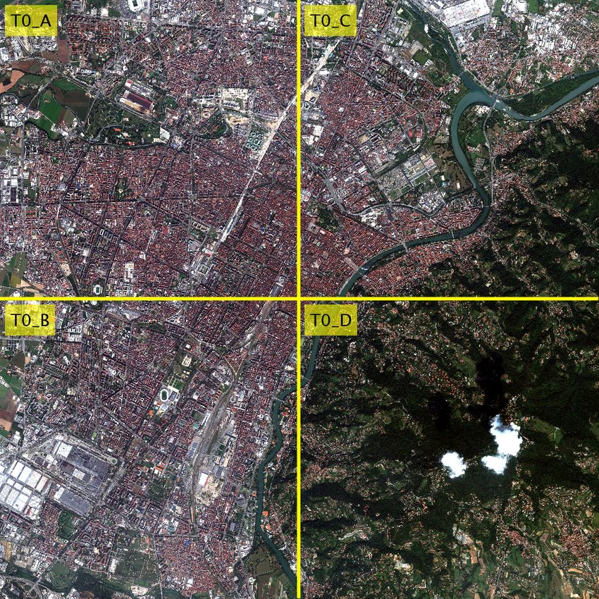
3

                                                                                                     2                           2    2
where λ is the characteristic scale, a measuring unit size,                 hence a log-log plot of σDM  A as a function of s = n1 + n2
and Df the fractal Hausdorff dimension:                                     yields a straight line with slope H.

                             Df = d − H       ,                       (2)   The scaling behaviour expected by Eq. (6) is illustrated
                                                                            in Fig. (2) where the 2d-DMA method is implemented
with d the Euclidean embedding dimension and H the                          on artificial fractal images, with different size and Hurst
Hurst exponent, ranging from 0 < H < 0.5 and 0.5 <                          exponent, generated by Cholesky-Levinson Factorization
H < 1, respectively for negatively and positively corre-                    (CLF) [36]. One of such surfaces with H = 0.2 is shown
lated random sets, and H = 0.5 corresponding to the                         in Fig. 2 (top panel). The σDM A values obtained for arti-
ordinary Brownian function, i.e. to fully uncorrelated                      ficial fractal surfaces with input Hurst exponent ranging
random sets.                                                                from 0.1 to 0.9, size 480×480 and 1024×1024 are plotted
As mentioned in the Introduction, the high-dimensional                      on log-log scales (middle and bottom panels). The differ-
detrended moving average (d-DMA) [34] is here applied                       ence between the input Hurst exponents and the DMA
to high-resolution WorldView-2 satellite images [35] to                     outcomes is negligible and decreases as the size of the
estimate the Hurst exponent H and fractal dimension                         surface increases.
Df of urban infrastructures. For the sake of clarity, the                   Real-world random data sets are not ideal fractals, as
main steps of the DMA method are briefly summarized                         those defined by the fractional Brownian functions fH (r),
below.                                                                      which are defined to exist at all scales. Being character-
Random fractal sets can be analytically described in                        ized by finite sizes that set upper and lower limits to the
terms of a scalar function fH (r) : Rd → R showing self-                    small and large observable scales, deviations from the ide-
similarity, with the Hurst exponent H as a parameter,                       ality should be expected. As a rule, real-world random
and correlation depending as a power law on the scale                       data sets are classified as fractals if their variance can be
λ (a measuring unit size, as in Eq. (1)). The power-law                     approximated by a power law over at least three decades
correlation is reflected by the variance:                                   of scales.
             2
            σH = [fH (r + λ) − fH (r)]2 ∝k λ k2H                      (3)   The high-dimensional Detrended Moving Average (DMA)
                                                                            has been applied to 2d and 3d artificial structures in
with r = (x1 , x2 , ..., xd ), λ = (λ1 , λ2 , ..., λd ) and k λ k=          [37, 38]. Evolution of rural landscape of Mangystan
(λ21 + λ22 + ... + λ2d )1/2 .                                               (Kazakhstan) and New Mexico (USA) monthly recorded
                                                                            from July 1982 to May 2012 by the multi-spectral Land-
The DMA algorithm operates via the definition of a
                                                                            Sat Thematic Mapper (TM) have been analysed in [39].
generalized high-dimensional variance σDM A of fH (r)
                                                                            Hurst exponents ranging between 0.21 ≤ H ≤ 0.30 and
around the moving average function f˜H (r) [34], that, for
                                                                            0.11 ≤ H ≤ 0.30, corresponding to fractal dimensions
d = 2, writes:
                                                                            between 1.70 ≤ Df ≤ 1.79 and 1.70 ≤ Df ≤ 1.89, have
                                                                            been found respectively for Mangystan and New Mexico.
   2                       1
  σDM A =
                                                                            Fractal dimension increases over time as man-made in-
               (N1 − n1max )(N2 − n2max )                             (4)   frastructures and build-up areas grow at the expenses of
                  N1   N2
                 X    X                                                     the natural landscape. In the next section, the fractal di-
               ×           [f (i1 , i2 ) − f˜n1 n2 (i1 , i2 )]2   ,
                                                                            mension of WorldView-2 satellite images of several cities
                  i1 =n1 i2 =n2
                                                                            will be estimated by using the two-dimensional Detrend-
                                                                            ing Moving Average algorithm (DMA).
with f˜n1 n2 (i1 , i2 ) given by:

                                1 −1 n
                               nX      2 −1
                        1            X                                                   III.   DATA AND RESULTS
f˜n1 n2 (i1 , i2 ) =         ×              f (i1 −k1 , i2 −k2 ) . (5)
                       n1 n2
                               k1 =0 k2 =0
                                                                            WorldView-2 [35] provides panchromatic imagery with
First, the average scalar field f˜n1 n2 (i1 , i2 ) is estimated             0.46m resolution, and eight-band multispectral imagery
over sub-arrays with different size n1 × n2 . The next                      with 1.84m resolution - representing one of the highest
step of the algorithm is the calculation of the difference                  available spaceborne resolutions. The subset European
f (i1 , i2 ) − f˜n1 ,n2 (i1 , i2 ) for each sub-array n1 × n2 . It can      Cities of the WorldView-2 database includes images of
been shown that Eq. (4) reduces to the form:                                several European cities and their hinterland, processed
                                                                            by the European Space Imaging GmbH during February
                               q            2H
                   2                                                        2011 to October 2013. The collection is related to ESA’s
                 σDM A ∼              2    2
                                     n1 + n2     = sH ,             (6)
                                                                            EO missions for the coverage of the urban areas in Eu-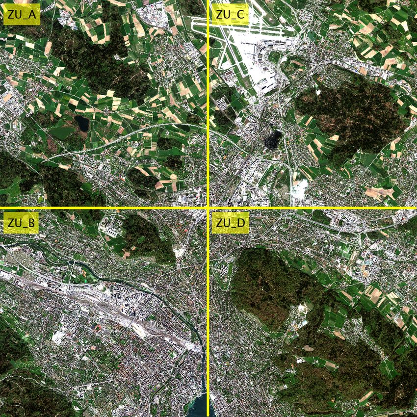
4

                                                                 rope and is referred as the Urban Atlas. With spatial
                                                                 resolutions of the order of 10m − 30m, LandSat and Sen-
                                                                 tinel satellites are very effective at mapping land coverage
                                                                 and criosphere by identifying the spectral signature and
                                                                 broadly classifying areas containing that spectral pat-
                                                                 tern. Multi-spectral satellite imagery with pixel resolu-
                                                                 tion of the order of 1m and less provide finer scale fea-
                                                                 tures able to investigate Earth crust phenomena at a mi-
                                                                 croscopic level. The high resolution might enable to dis-
                                                                 criminate fine details of Land Use/Land Cover (LULC)
                                                                 such as farmland, urban areas, quality of road surfaces,
                                                                 and health of plants. The multiple spectral bands yield
                                                                 inter-band spectral information to discriminate features
                                                                 of texture [40, 41].

                                                                 Samples of the analysed urban areas are shown in the
                                                                 top panels of Figs. 3-6. The images are 1080 × 1080 pix-
                                                                 els large. Sub-images are obtained by dividing the main
                                                                 image into four squares of size 540 × 540, delimited by
                                                                 yellow lines and labelled by A, B, C, D. Here, we report
                                                                 results obtained on a single band, i.e. the red band. Re-
                                                                 sults obtained for green and blue bands, different sectors
                                                                 and other cities will be reported in a forthcoming work.
                                                                 Before implementing the DMA algorithm, raw data are
                                                                 converted from the uint8 to the double format For each
                                                                 sub-image, the algorithm is implemented separately to
                                                                 grasp the variability of the scaling properties of different
                                                                 areas (partially mountainous, suburban, centrally located
                                                                 areas).
                                                                                           2
                                                                 Log-log values of the σDM    A are plotted in the bottom
                                                                 panels of Figs. 3-6. Deviations from the fully linear
                                                                 trend, that would be expected for an ideal fractal, can
                                                                 be observed particularly at the low scales (small s val-
                                                                                    2
                                                                 ues) where the σDM    A drops down. In order to account
                                                                 for and evaluate the extent of non-ideality and the de-
                                                                 viations at the extreme scales, multiple computational
                                                                 steps are implemented. Regressions are computed for
                                                                 the first three decades (2 < s < 5), the last three decades
                                                                 (5.5 < s < 8.5) and the whole range of scales, providing
                                                                 three estimates of the Hurst exponent (respectively H1 ,
                                                                 H2 and H). The last three decades and the whole range
FIG. 2.     Fractional Brownian surface with size 512 × 512      provide quite close and accurate values of the Hurst ex-
and Hurst exponent H = 0.2 generated via FRACLAB [36]            ponents (H and H2 ) with excellent goodness of fit as
                         2
(Top). Log-log plots of σDM  A results for Fractional Brownian   indicated by the high R2 values. Higher values of the
surfaces with Hurst exponent H = 0.1, 0.2, 0.3, ..., 0.9. Each   slope are obtained for the first decade (H1 ). Being the
color refers to DM A results and to Hurst exponent estimates     pixel resolution of the order of 1.84m (single band), the
H for a different Fractional Brownian surface. The Hurst         minimum area detectable by the DMA algorithm is of
exponent estimates reported in the legend are obtained as        the order of 1.84m × 1.84m, a much smaller value than
                                                          2
the slope of the regression line by least squares of ln σDM A.   the minimal average urban block size (about 10m×10m).
Results are reported for Fractional Brownian surfaces of size
                                                                 Thus fewer elementary random built-up components are
480 × 480 (middle panel) and 1024 × 1024 (bottom panel).
                                                                 found and counted at the smallest scales compared to the
                                                                 number that would be expected for an ideal self-similar
                                                                 structure.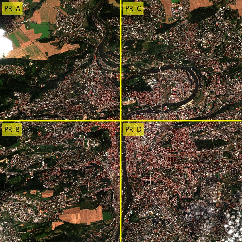
5

                                                                    urbanised areas (Torino hills). In Table I further results
                                                                    are reported for other Turin areas (image N45-037 and
                                                                    N45-124).

FIG. 3. Image 45-024 (Torino) downloaded from the Urban
Atlas collection of the largest European Cities of WorldView-
2 satellite images [35]. The image is multi-spectral with size
1080 × 1080. Yellow lines divide the image into 4 sub-images
                                                            2
A, B, C, D of size 540 × 540 (Top). Log-log plots of σDM       A
                                                                    FIG. 4. Same as for Fig. 3 but for image 48-181 (Vienna).
for sub-images A, B, C, D. The DMA results refer to the
red band only. Hurst Exponent estimates H, obtained as the
slope of the regression line by least squares, are calculated for   Image N 48-181 (Vienna) is shown in Fig. 4 (top panel)
                                                                              2
each sub-image. Goodness of fit is evaluated by R2 (Bottom)         and the σDM   A results are plotted in log-log scale (bottom
                                                                    panels). Sections A, B and C are highly urbanized areas,
                                                                    while Section D is less urbanized. This is reflected in the
                                                                    Hurst exponent estimates, which tends to be lower for
Image N45-024 (Turin) is shown in Fig. 3 (top panel).
                     2
                                                                    urbanized areas. H2 ranges between 0.09÷0.17, H ranges
Log-log results of σDM  A are plotted for each sub-image            between 0.12 ÷ 0.20, while H1 ranges between 0.22 ÷ 0.27
A, B, C, D for the whole range of s scales (bottom pan-
                                                                    (Table I). In Table I further results are reported for other
els). The slope is estimated by ordinary linear regression
                                                                    areas of Vienna (image N48-006 and N48-465).
over three different ranges of s values. H1 , H and H2
corresponding respectively to the first, intermediate and           Image N 47-377 (Zurich) is shown in Fig.5 (top panel)
                                                                              2
last decades of s are reported in Table I. H2 ranges be-            and the σDM  A results are plotted in log-log scale (bot-
tween 0.10 ÷ 0.15, H ranges between 0.12 ÷ 0.16, while              tom panels). The most densely urbanized area looks
H1 ranges between 0.23 ÷ 0.24. The Hurst exponent of                Section B, while the least Section A; overall, the city
section D is the highest and indeed corresponds to less             of Zurich seems more heterogeneous compared to Turin
6

FIG. 5. Same as Fig. 3 but for the image 47-377 (Zurich).   FIG. 6. Same as Fig. 3 but for the image N50-090 (Prague).

(Fig. 3) and Vienna (Fig. 4). Large wooded areas in-        of Tables I for the sector A,B,C,D of the above described
terrupt frequently the urbanized grid. This is reflected    images. Df values have been calculated by introducing
in the Hurst exponent, which takes higher and less di-      the value H2 in the relationship Eq. 2. Df values with
versified values than for Torino and Vienna. H2 ranges      H and H1 can be easily obtained as well.
between 0.10 ÷ 0.20, H ranges between 0.12 ÷ 0.22, while
H1 ranges between 0.22 ÷ 0.28 (Table I). Further results
are reported for other areas of Zurich (images N47-167
and N48-230) in Table I.                                                      IV.   DISCUSSION

The image N50-090 of the city of Prague is shown in         In this section, the values of H and Df obtained in Sec-
                        2
Fig. 6 (top panel) and σDM                                  tion III and summarized in Table I, will be compared
                           A results are reported in log-
log scale (bottom panels) for each of the four sections     with those reported in previous works [9–17]. Further-
of the whole image. H2 ranges between 0.11 ÷ 0.16, H        more, the urban scaling exponents β will be estimated
ranges between 0.14÷0.17, while H1 takes the value 0.26.    by introducing the numerical results of Df into the rela-
Further results are reported for other areas of Prague      tionships linking β and Df worked out in [3–5]. For the
(images N50-045 and N49-908) in Table I.                    sake of the discussion, a brief summary of previous stud-
                                                            ies dealing with fractal measurements and scaling models
The fractal dimension Df is reported in the last column     of urban areas is reported here below.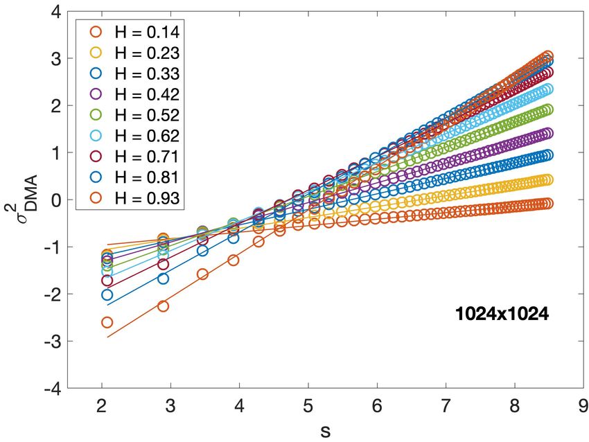
7

                       Torino      H1      H     H2      R2    Df       Vienna      H1      H     H2      R2    Df
                               A   0.23   0.12   0.10   0.93   1.90             A   0.23   0.13   0.11   0.94   1.89
                               B   0.23   0.13   0.11   0.95   1.89             B   0.24   0.15   0.13   0.97   1.87
                      N 45-024                                         N 48-181
                               C   0.24   0.13   0.11   0.94   1.89             C   0.22   0.12   0.09   0.93   1.90
                               D   0.25   0.16   0.15   0.97   1.85             D   0.27   0.20   0.17   0.98   1.83
                               A   0.31   0.30   0.32   1.00   1.68             A   0.33   0.26   0.23   0.99   1.77
                               B   0.27   0.25   0.27   0.99   1.73             B   0.38   0.30   0.27   0.99   1.73
                      N 45-037                                         N 48-006
                               C   0.28   0.23   0.23   0.99   1.77             C   0.33   0.29   0.27   1.00   1.73
                               D   0.33   0.30   0.31   1.00   1.69             D   0.33   0.26   0.22   0.99   1.78
                               A   0.30   0.28   0.30   1.00   1.70             A   0.41   0.30   0.27   0.99   1.73
                               B   0.27   0.22   0.23   0.99   1.77             B   0.39   0.32   0.31   1.00   1.69
                      N 45-124                                         N 48-465
                               C   0.25   0.16   0.13   0.97   1.87             C   0.40   0.29   0.26   0.99   1.74
                               D   0.26   0.17   0.15   0.98   1.85             D   0.40   0.28   0.24   0.98   1.76

                       Zurich      H1      H     H2      R2    Df       Prague      H1      H     H2      R2    Df
                               A   0.28   0.22   0.20   0.99   1.80             A   0.26   0.17   0.16   0.97   1.84
                               B   0.27   0.19   0.17   0.98   1.83             B   0.26   0.15   0.12   0.95   1.88
                      N 47-377                                         N 50-090
                               C   0.23   0.12   0.10   0.93   1.90             C   0.26   0.16   0.14   0.96   1.86
                               D   0.22   0.14   0.12   0.96   1.88             D   0.26   0.14   0.11   0.93   1.89
                               A   0.26   0.19   0.16   0.98   1.84             A   0.25   0.18   0.17   0.99   1.83
                               B   0.27   0.20   0.19   0.99   1.81             B   0.24   0.14   0.12   0.95   1.88
                      N 47-167                                         N 50-045
                               C   0.28   0.23   0.23   0.99   1.77             C   0.25   0.19   0.19   0.99   1.81
                               D   0.26   0.18   0.16   0.98   1.84             D   0.26   0.21   0.21   0.99   1.79
                               A   0.28   0.23   0.21   0.99   1.79             A   0.29   0.24   0.24   0.99   1.76
                               B   0.27   0.21   0.19   0.99   1.81             B   0.34   0.32   0.32   1.00   1.68
                      N 47-230                                         N 49-908
                               C   0.29   0.23   0.21   0.99   1.79             C   0.36   0.32   0.33   1.00   1.67
                               D   0.27   0.21   0.18   0.99   1.82             D   0.33   0.29   0.30   1.00   1.70

TABLE I. Hurst exponents estimated for the WorldView-2 satellite images 45-024, 45-037, 45-124 (Torino); 48-181, 48-006,
48-465 (Vienna); 47-377, 47-230, 47-167 (Zurich); 50-090, 50-045, 49-908 (Prague). The Hurst exponents H1 H and H2 have
been obtained by implementing the 2d-Detrending Moving Average algorithm over the first, whole and last range of decades as
summarised in Section II. For each image the Hurst exponent is estimated for 4 cross-sections (different urban areas) labelled
A, B, C, D as shown in Fig. 3 for the image 45-024. Last column reports the estimates of the fractal dimension by using
Df = d − H with the Hurst exponents H2 and d = 2. Using the Hurst exponents results in the second column, referred to as
H, alternative but similar values of Df can be obtained.

The fractal dimension Df of cities has been estimated                 1.62 ≤ Df ≤ 1.80 [15]. Fractal dimensions of satellite im-
by approaches as diverse as box-counting, radial method               ages of cities are obtained by (i) isarithm, (ii) triangular
[11–14] isarithm, variogram [15–17]. With embedding di-               prism and (iii) variogram ranging respectively between
mension d = 2 and d = 3, the fractal dimension Df takes               (i) 2.80 ≤ Df ≤ 3.00; (ii) 2.60 ≤ Df ≤ 2.80, for urban,
value respectively in the range 1.0÷2.0 and 2.0÷3.0. The              forest and grass, 2.30 ≤ Df ≤ 2.80 for cropland and pas-
Hurst exponent takes a unique value regardless of d allow-            ture; 2.20 ≤ Df ≤ 2.60 for water; (iii) 2.80 ≤ Df ≤ 3.00
ing the comparison of results obtained by different meth-             for cropland and water; Df ≥ 3.00 for urban, forest and
ods. Fractal dimensions ranging between 1.28 ≤ Df ≤                   grass [16]. The triangular prism yields lower values of Df
1.70 have been reported for Omaha and New York City in                compared to those obtained by isarithm and variogram
[11], between 1.44 ≤ Df ≤ 1.62, and 1.68 ≤ Df ≤ 1.50,                 methods. The images analysed by triangular prism date
for Belgium’s 18 largest cities in [12]. Values in the range          back to 1975, while the other images were acquired in
1 ≤ Df < 1.26, for dispersed areas, 1.26 ≤ Df < 1.54                  2000 (isarithm and variogram). After 25 years, the city
for new seeds of urbanised areas, 1.54 ≤ Df ≤ 2 for                   had become a large metropolis where roads, highways,
densely urbanized and consolidated areas are reported                 and buildings filled the area. Such changes in the urban
for Lisbon in Ref. [13]. Several mega-cities and mining               landscape can reasonably explain the increased value of
cities of China are investigated over different periods: the          Df and the corresponding decrease of H. Fractal di-
fractal dimension ranges between 1.57 ≤ Df ≤ 1.74 in                  mension of red band satellite images of the Indianapo-
1990, and 1.57 ≤ Df ≤ 1.78 in 2000 [14] and between                   lis area ranges respectively between 2.72 ≤ Df ≤ 2.82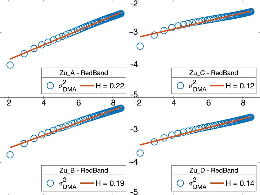
8
Ref. [2] [3] [4] [5] size, with scaling exponents respectively for the infras-
Df γ Df
βi [0.74, 0.92] 1− d(d+Df ) Df Dp
tructural and socio-economic quantities:
βs [1.01, 1.33] 1+
Df
2− γ
2−
Df γ γ
d(d+Df ) Df Dp βi = βs = 2 − , (8)
Df Df
with γ varying in the range 1.0 ÷ 1.5 and γ = 1.0 cor-
responds to the Newtonian gravitational law in d = 2.
In the long-range interaction regime γ/Df < 1, βs >
1 implying that superlinear socio-economic scaling be-
haviour occurs when the individuals can interact with
all other individuals of the city. In Ref. [5] a three-
dimensional building infrastructure is considered with
the socio-economic interactions occurring in a 3D fractal
cloud. The scaling exponents for the infrastructures and
the socio-economic activities are written respectively:
Df Df
βi = βs = 2 − . (9)
Dp Dp
For the ease of the discussion, Eqs. (7-9) are gathered to-
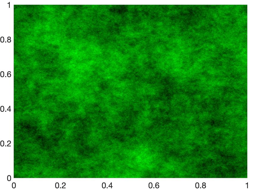
FIG. 7. Range of the empirical values for βi and βs reported
gether in the top panel of Fig. 7 (third, fourth and fifth
in Ref. [2] (second column). Analytical expression of the ex- columns) with the empirical values of βi and βs (second
ponents βi and βs deduced in Refs. [3–5] (respectively third, column) reported in [2]. The derivatives of the scaling
fourth and fifth columns). Plot of βs (filled symbols) and βi exponents βi and βs with respect to Df yield respec-
(hollow symbols) as defined by Eqs. (7) (red circle), Eqs. (8) tively: ∂βs /∂Df = 1/(d + Df )2 ; ∂βs /∂Df = γ/Df2 ;
(blue square) Eqs. (9) (green diamond). A different depen- ∂βs /∂Df = −1/(1 + Df )2 (the derivatives ∂βi /∂Df are
dence of the exponents on the fractal dimension is observed: the same but with opposite sign). The exponents βi and
βs increases (βi decreases) very slowly with the fractal dimen- βs exhibit a different dependence on Df , as Fig. 7 also
sion Df according to Ref. [3]; a stronger increase (decrease) shows. In particular, the exponent βs increases (βi de-
is found according to Ref. [4]; whereas βs decreases (βi in-
creases) very slowly with the fractal dimension Df ac-
creases) with Df according to Ref.[5].
cording to Eqs. (7). A steeper increase of βs (decrease
of βi ) is found according to the Eqs. (8) which exhibit
(isarithm), 2.78 ≤ Df ≤ 2.93 (triangular prism), and an interesting behaviour: at Df = 1.5, βi and βs be-
2.88 ≤ Df ≤ 2.96 (variogram) Ref. [17]. On average the come respectively larger and smaller than 1. The inver-
H values obtained by using satellite images are smaller sion can be related to the different constraints posed by
than those obtained by using traditional data sets as car- a urban area mostly distributed along a one-dimensional
tographic maps. geometrical structure, with fractal dimension Df → 1.
Such topological constraint implies that the cost of the
To further substantiate our study, the values of the Hurst physical infrastructure exceeds the socioeconomic urban
exponent H and of the fractal dimension Df of the satel- organization advantage. Df → 2 corresponds to a com-
lite images as those in Figs. 3-6 will be validated against pact urban structure almost regularly distributed over
the the relationships linking β and Df deduced in Refs. a two-dimensional surface, where the cost of the infras-
[3–5] briefly recalled below. tructure are fully compensated by the socio-economic de-
Under the assumption of incremental network growth velopment advantage. Surprisingly. βs decreases (βi in-
and bounded human effort, infrastructural and the socio- creases) with Df according to Eqs. (9) and Ref. [5]. In
economic features are written in Ref. [3] as power laws this case, the behaviour of βs does not exhibit the increas-
of the population size respectively with exponents: ing dependence on Df expected on account of previous
studies.
Df Df
βi = 1 − βs = 1 + (7) The fractal dimension values (ranging between 1.6 ≤
d(d + Df ) d(d + Df )
Df ≤ 1.8 and 1 < Df < 2) used for the scaling law
In Ref. [4], the interaction strength between individuals estimates were taken from third party sources in [3–5].
is modelled in terms of a scalar field varying inversely In this work, the exponents βi and βs are calculated by
with the distance and the total interaction intensity is introducing the values of Df (Table I) into the Eqs. (7-
obtained in the form of a power law of the population 9). Values are shown in Table II. Columns from 3 to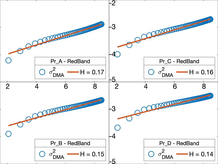
9

                              Ref.                 [3]                          [4]                          [5]
                            Vienna      A      B         C    D      A      B         C    D      A      B         C    D
                                  βi   0.76   0.76   0.76    0.76   0.80   0.81   0.80    0.83   0.65   0.65   0.65    0.64
                          N48-181
                                  βs   1.24   1.24   1.24    1.24   1.20   1.20   1.20    1.17   1.35   1.35   1.35    1.36
                                  βi   0.76   0.77   0.77    0.76   0.85   0.87   0.87    0.84   0.64   0.63   0.63    0.64
                         N48-006
                                  βs   1.23   1.23   1.23    1.23   1.15   1.13   1.13    1.16   1.36   1.37   1.37    1.36
                                  βi   0.77   0.77   0.77    0.77   0.87   0.89   0.86    0.85   0.63   0.63   0.63    0.64
                         N 48-465
                                  βs   1.23   1.23   1.23    1.23   1.13   1.11   1.14    1.15   1.37   1.37   1.36    1.36
                            Prague      A      B         C    D      A      B         C    D      A      B         C    D
                                  βi   0.76   0.76   0.76    0.76   0.82   0.81   0.81    0.80   0.65   0.65   0.65    0.65
                         N 50-090
                                  βs   1.24   1.24   1.24    1.24   1.18   1.19   1.18    1.19   1.35   1.35   1.35    1.35
                                  βi   0.76   0.76   0.76    0.76   0.82   0.80   0.83    0.84   0.65   0.65   0.64    0.64
                         N 50-045
                                  βs   1.24   1.24   1.24    1.24   1.18   1.20   1.17    1.16   1.35   1.35   1.36    1.36
                                  βi   0.77   0.77   0.77    0.77   0.85   0.89   0.89    0.88   0.64   0.63   0.62    0.63
                         N 50-908
                                  βs   1.23   1.23   1.23    1.23   1.15   1.11   1.10    1.12   1.36   1.37   1.37    1.37
                            Torino      A      B         C    D      A      B         C    D      A      B         C    D
                                  βi   0.76   0.76   0.76    0.76   0.79   0.79   0.79    0.81   0.65   0.65   0.65    0.65
                         N 45-024
                                  βs   1.24   1.24   1.24    1.24   1.21   1.21   1.21    1.19   1.34   1.35   1.35    1.35
                                  βi   0.77   0.77   0.76    0.77   0.89   0.87   0.85    0.89   0.63   0.63   0.64    0.63
                         N 45-037
                                  βs   1.23   1.23   1.23    1.23   1.11   1.13   1.15    1.11   1.37   1.37   1.36    1.37
                                  βi   0.77   0.76   0.76    0.76   0.88   0.85   0.80    0.81   0.63   0.64   0.65    0.65
                         N 45-124
                                  βs   1.23   1.23   1.24    1.24   1.12   1.15   1.20    1.19   1.37   1.36   1.35    1.35
                            Zurich      A      B         C    D      A      B         C    D      A      B         C    D
                                  βi   0.76   0.76   0.76    0.76   0.83   0.82   0.79    0.80   0.64   0.65   0.65    0.65
                         N 47-377
                                  βs   1.24   1.24   1.24    1.24   1.17   1.18   1.21    1.20   1.36   1.35   1.34    1.35
                                  βi   0.76   0.76   0.76    0.76   0.81   0.83   0.85    0.81   0.65   0.64   0.64    0.65
                         N 47-167
                                  βs   1.24   1.24   1.23    1.24   1.18   1.17   1.15    1.18   1.35   1.36   1.36    1.35
                                  βi   0.76   0.76   0.76    0.76   0.84   0.83   0.84    0.82   0.64   0.64   0.64    0.64
                         N 47-230
                                  βs   1.24   1.24   1.24    1.24   1.16   1.17   1.16    1.18   1.36   1.36   1.36    1.35

TABLE II. Scaling exponents βi and βs obtained by using the values of Df reported in Table I. The values for the sections A,
B, C, D are obtained by using Eqs. (7), Eqs. (8) with γ = 1.5 and Eqs. (9), with Dp = Df + 1.

6 show the values obtained by Eqs. (7); Eqs. (8) with                      and suburban areas. In particular, the Hurst exponent
γ = 1.5 correspond to columns from 7 to 10); Eqs. (9)                      H (resp., the fractal dimension Df ) is smaller (larger)
with Dp = Df + 1 correspond to columns from 11 to                          for highly urbanized areas and larger (smaller) for de-
14. The analyzed areas have infrastructures scaling sub-                   tached rural areas. The Hurst exponent H of several
linearly and socio-economic interactions scaling super-                    large European cities has been estimated by implement-
linearly with exponents in the range of empirical values                   ing the Detrended Moving Average algorithm on high
according to Ref.[2] when Eqs. (7) and Eqs. (8) are used.                  resolution remotely sensed images (WorldView-2 Urban
The values of the exponent yielded by Eqs. (9) systemat-                   Atlas database). The values of H are linked to the frac-
ically exceed the expected values. The values are plotted                  tal dimension Df through the relationship (2). Our es-
in Fig. 8, where the range of empirical values (column 2                   timates provide 0.10 ≤ H ≤ 0.30 for the Hurst expo-
of the Table in 7) are also indicated by thin horizontal                   nent, which correspond to fractal dimensions ranging be-
lines.                                                                     tween 1.65 ≤ Df ≤ 1.90. Interestingly, we obtain slightly
                                                                           smaller Hurst exponent and higher fractal dimension on
                                                                           average with respect to the estimates of the urban frac-
                                                                           tal dimensions reported in [11–14]. Our values of the
                 V.    CONCLUSIONS                                         Hurst exponent are closer to those provided in Refs. [15–
                                                                           17]. This result seems to suggest that highly reproducible
                                                                           values are obtained when satellite images are used as op-
This work enriches the existing literature on two fronts.                  posed to those provided by other data sets.
First, it provides a new method for urban classification
capable of distinguishing different areas such as urban                    Second, the manuscript demonstrates that a geometri-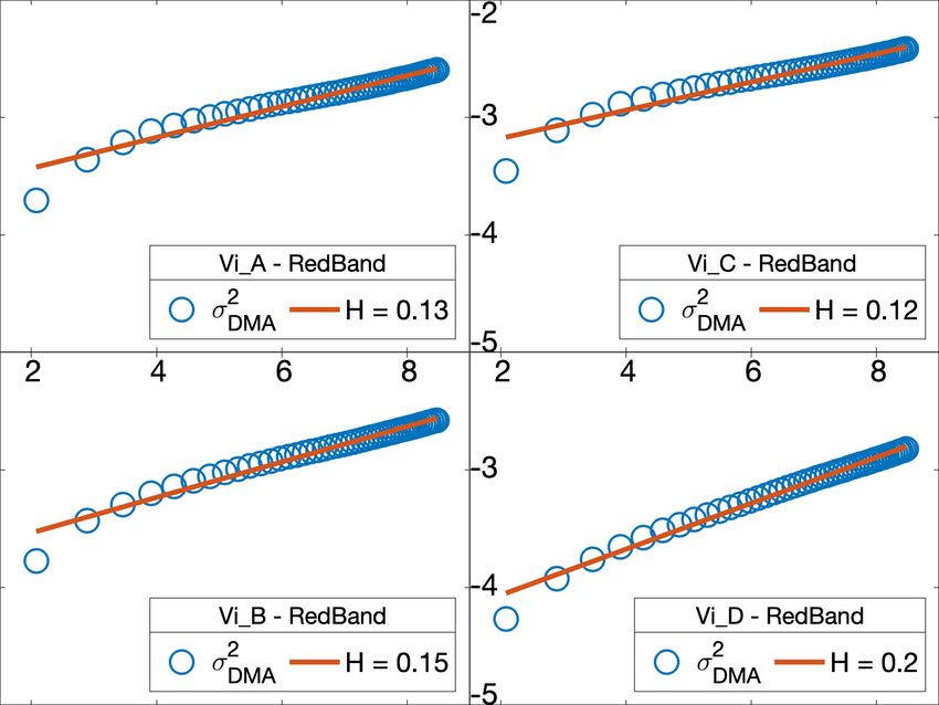
10

FIG. 8. Experimental exponents βs (filled symbols) and βi (hollow symbols) as defined by Eqs. (7) (circle), Eqs. (8) (square)
and Eqs. (9) (diamond) for different areas of Torino, Zurich, Vienna and Prague. A different dependence of the exponents on
the fractal dimension is observed.

cal approach to urban scaling theory, which exploit the            used alone or in combination with other measures and
statistical structure of high resolution satellite images of       approaches to provide significant new insights in urban
cities, provides robust estimates and validation of urban          scaling model analysis and in designing the related needs
scaling laws. A rich theory has developed a number of              for intervention and policy-making activities.
models that describe the characteristic power law behav-
ior of features exhibiting super-linear or sub-linear scaling
respectively for socio-economic and infrastructural vari-
ables. Interestingly, for the quantification of such for-                         ACKNOWLEDGMENTS
mulae, the theoretical framework relies on fractal mea-
sures. By using the definitions of the scaling exponents           This work received financial support from the Fu-
reported in the table at the top of Figure 7, βi and βs            turICT2.0 project (a FLAG-ERA Initiative within the
can be calculated. The results for the images N45-024,             Joint Transnational Calls 2016, Grant Number: JTC-
N48-181, N47-377 and N50-090 of the cities of Turin, Vi-           2016-004) and from the SIP project (Italian Ministry of
enna, Zurich and Prague are reported in Table II and               Economic Development (MISE) Programme on "Emerg-
plotted in Figure 8. Thus, the proposed method can be              ing Technologies in the context of 5G").

 [1] Jian Gao, Yi-Cheng Zhang, and Tao Zhou. Computa-                   Society Open Science, 4(3):160926, 2017.
     tional socioeconomics. Physics Reports, 817:1–104, 2019.       [5] Carlos Molinero and Stefan Thurner. How the geometry
 [2] Luís MA Bettencourt, José Lobo, Dirk Helbing, Chris-               of cities determines urban scaling laws. Journal of the
     tian Kühnert, and Geoffrey B West. Growth, innovation,             Royal Society Interface, 18(176):20200705, 2021.
     scaling, and the pace of life in cities. Proceedings of the    [6] Juval Portugali. Self-organization and the city. Springer
     national academy of sciences, 104(17):7301–7306, 2007.             Science & Business Media, 2012.
 [3] Luís MA Bettencourt. The origins of scaling in cities.         [7] Hermann Haken and Juval Portugali. Urban scaling, ur-
     Science, 340(6139):1438–1441, 2013.                                ban regulatory focus and their interrelations. Synergetic
 [4] Fabiano L Ribeiro, Joao Meirelles, Fernando F Ferreira,            Cities: Information, Steady State and Phase Transition:
     and Camilo Rodrigues Neto. A model of urban scaling                Implications to Urban Scaling, Smart Cities and Plan-
     laws based on distance dependent interactions. Royal               ning, pages 199–215, 2021.
11
[8] B.B. Mandelbrot. Fractals: Form, Chance and Dimen- urban scaling laws. Computers, environment and urban
sion. Freeman, 1977. systems, 63:80–94, 2017.
[9] Michael Batty and Paul A Longley. Fractal-based de- [26] Elsa Arcaute, Erez Hatna, Peter Ferguson, Hyejin Youn,
scription of urban form. Environment and planning B: Anders Johansson, and Michael Batty. Constructing
Planning and Design, 14(2):123–134, 1987. cities, deconstructing scaling laws. Journal of the royal
[10] Pierre Frankhauser. The fractal approach. a new tool for society interface, 12(102):20140745, 2015.
the spatial analysis of urban agglomerations. Population: [27] Diego Rybski, Elsa Arcaute, and Michael Batty. Urban
an english selection, pages 205–240, 1998. scaling laws, 2019.
[11] Guoqiang Shen. Fractal dimension and fractal growth of [28] Christopher D Elvidge, Kimberley E Baugh, Eric A
urbanized areas. International Journal of Geographical Kihn, Herbert W Kroehl, Ethan R Davis, and Chris W
Information Science, 16(5):419–437, 2002. Davis. Relation between satellite observed visible-near
[12] Cécile Tannier and Isabelle Thomas. Defining and char- infrared emissions, population, economic activity and
acterizing urban boundaries: A fractal analysis of theo- electric power consumption. International Journal of Re-
retical cities and belgian cities. Computers, Environment mote Sensing, 18(6):1373–1379, 1997.
and Urban Systems, 41:234–248, 2013. [29] Steeve Ebener, Christopher Murray, Ajay Tandon, and
[13] Sara Encarnação, Marcos Gaudiano, Francisco C San- Christopher C Elvidge. From wealth to health: modelling
tos, José A Tenedório, and Jorge M Pacheco. Fractal the distribution of income per capita at the sub-national
cartography of urban areas. Scientific Reports, 2(1):1–5, level using night-time light imagery. international Jour-
2012. nal of health geographics, 4(1):1–17, 2005.
[14] Yanguang Chen. A set of formulae on fractal dimension [30] Dave Donaldson and Adam Storeygard. The view from
relations and its application to urban form. Chaos, Soli- above: Applications of satellite data in economics. Jour-
tons & Fractals, 54:150–158, 2013. nal of Economic Perspectives, 30(4):171–98, 2016.
[15] Charles W Emerson, Nina Siu-Ngan Lam, and Dale A [31] Neal Jean, Marshall Burke, Michael Xie, W Matthew
Quattrochi. A comparison of local variance, fractal di- Davis, David B Lobell, and Stefano Ermon. Combin-
mension, and moran’s i as aids to multispectral image ing satellite imagery and machine learning to predict
classification. International Journal of Remote Sensing, poverty. Science, 353(6301):790–794, 2016.
26(8):1575–1588, 2005. [32] Thilo Wellmann, Angela Lausch, Erik Andersson, Sonja
[16] Bingqing Liang, Qihao Weng, and Xiaohua Tong. An Knapp, Chiara Cortinovis, Jessica Jache, Sebastian
evaluation of fractal characteristics of urban landscape Scheuer, Peleg Kremer, André Mascarenhas, Roland
in indianapolis, usa, using multi-sensor satellite images. Kraemer, et al. Remote sensing in urban planning: Con-
International journal of remote sensing, 34(3):804–823, tributions towards ecologically sound policies? Land-
2013. scape and Urban Planning, 204:103921, 2020.
[17] Bingqing Liang and Qihao Weng. Characterizing ur- [33] Marshall Burke, Anne Driscoll, David B Lobell, and Ste-
ban landscape by using fractal-based texture informa- fano Ermon. Using satellite imagery to understand and
tion. Photogrammetric Engineering & Remote Sensing, promote sustainable development. Science, 371(6535),
84(11):695–710, 2018. 2021.
[18] Hernán D Rozenfeld, Diego Rybski, Xavier Gabaix, and [34] Anna Carbone. Algorithm to estimate the hurst expo-
Hernán A Makse. The area and population of cities: New nent of high-dimensional fractals. Physical Review E,
insights from a different perspective on cities. American 76(5):056703, 2007.
Economic Review, 101(5):2205–25, 2011. [35] Urban Atlas, last visit on 07/2021. The ESA third party
[19] David Levinson. Network structure and city size. PloS mission collection of the largest European urban areas
one, 7(1):e29721, 2012. recorded by the WorldView-2 satellite https://tpm-ds.
[20] K Yakubo, Y Saijo, and D Korošak. Superlinear and sub- eo.esa.int/oads/access/collection/WorldView-2.
linear urban scaling in geographical networks modeling [36] FRACLAB, last visit on 07/2021. We use the CLF algo-
cities. Physical Review E, 90(2):022803, 2014. rithm included in the package FRACLAB downloadable
[21] Hao Wu, David Levinson, and Somwrita Sarkar. How at https://project.inria.fr/fraclab/.
transit scaling shapes cities. Nature Sustainability, [37] Anna Carbone, Bernardino M Chiaia, Barbara Frigo,
2(12):1142–1148, 2019. and Christian Türk. Snow metamorphism: A fractal ap-
[22] Marc Keuschnigg, Selcan Mutgan, and Peter Hedström. proach. Physical Review E, 82(3):036103, 2010.
Urban scaling and the regional divide. Science advances, [38] Christian Türk, Anna Carbone, and Bernardino M Chi-
5(1):eaav0042, 2019. aia. Fractal heterogeneous media. Physical Review E,
[23] Lei Dong, Zhou Huang, Jiang Zhang, and Yu Liu. Un- 81(2):026706, 2010.
derstanding the mesoscopic scaling patterns within cities. [39] Juan C Valdiviezo-N, Raul Castro, Gabriel Cristóbal,
Scientific reports, 10(1):1–11, 2020. and Anna Carbone. Hurst exponent for fractal character-
[24] Eduardo G Altmann. Spatial interactions in urban scal- ization of landsat images. In Remote sensing and model-
ing laws. Plos one, 15(12):e0243390, 2020. ing of ecosystems for sustainability Xi, volume 9221, page
[25] Clémentine Cottineau, Erez Hatna, Elsa Arcaute, and 922103. International Society for Optics and Photonics,
Michael Batty. Diverse cities or the systematic paradox of 2014.12
[40] Mario Arreola-Esquivel, Carina Toxqui-Quitl, Maricela 13(14):2777, 2021.
Delgadillo-Herrera, Alfonso Padilla-Vivanco, Gabriel [41] Abdelmounaime Safia and Dong-Chen He. Multiband
Ortega-Mendoza, and Anna Carbone. Non-binary snow compact texture unit descriptor for intra-band and inter-
index for multi-component surfaces. Remote Sensing, band texture analysis. ISPRS journal of photogrammetry
and remote sensing, 105:169–185, 2015.You can also read