Beyond 2D landslide inventories and their rollover: synoptic 3D inventories and volume from repeat lidar data - Earth ...
←
→
Page content transcription
If your browser does not render page correctly, please read the page content below

Earth Surf. Dynam., 9, 1013–1044, 2021
https://doi.org/10.5194/esurf-9-1013-2021
© Author(s) 2021. This work is distributed under
the Creative Commons Attribution 4.0 License.

            Beyond 2D landslide inventories and their rollover:
                synoptic 3D inventories and volume from
                            repeat lidar data
                                 Thomas G. Bernard, Dimitri Lague, and Philippe Steer
                      Univ. Rennes, CNRS, Géosciences Rennes – UMR 6118, 35000 Rennes, France
                        Correspondence: Thomas G. Bernard (thomas.bernard@univ-rennes1.fr)

                              Received: 2 September 2020 – Discussion started: 15 September 2020
                           Revised: 29 June 2021 – Accepted: 12 July 2021 – Published: 26 August 2021

      Abstract. Efficient and robust landslide mapping and volume estimation is essential to rapidly infer landslide
      spatial distribution, to quantify the role of triggering events on landscape changes, and to assess direct and
      secondary landslide-related geomorphic hazards. Many efforts have been made to develop landslide mapping
      methods, based on 2D satellite or aerial images, and to constrain the empirical volume–area (V –A) relationship
      which, in turn, would allow for the provision of indirect estimates of landslide volume. Despite these efforts,
      major issues remain, including the uncertainty in the V –A scaling, landslide amalgamation and the underdetec-
      tion of landslides. To address these issues, we propose a new semiautomatic 3D point cloud differencing method
      to detect geomorphic changes, filter out false landslide detections due to lidar elevation errors, obtain robust
      landslide inventories with an uncertainty metric, and directly measure the volume and geometric properties of
      landslides. This method is based on the multiscale model-to-model cloud comparison (M3C2) algorithm and
      was applied to a multitemporal airborne lidar dataset of the Kaikōura region, New Zealand, following the Mw
      7.8 earthquake of 14 November 2016.
         In a 5 km2 area, the 3D point cloud differencing method detects 1118 potential sources. Manual labeling of
      739 potential sources shows the prevalence of false detections in forest-free areas (24.4 %), due to spatially cor-
      related elevation errors, and in forested areas (80 %), related to ground classification errors in the pre-earthquake
      (pre-EQ) dataset. Combining the distance to the closest deposit and signal-to-noise ratio metrics, the filtering
      step of our workflow reduces the prevalence of false source detections to below 1 % in terms of total area
      and volume of the labeled inventory. The final predicted inventory contains 433 landslide sources and 399 de-
      posits with a lower limit of detection size of 20 m2 and a total volume of 724 297 ± 141 087 m3 for sources
      and 954 029 ± 159 188 m3 for deposits. Geometric properties of the 3D source inventory, including the V –A
      relationship, are consistent with previous results, except for the lack of the classically observed rollover of the
      distribution of source area. A manually mapped 2D inventory from aerial image comparison has a better lower
      limit of detection (6 m2 ) but only identifies 258 landslide scars, exhibits a rollover in the distribution of source
      area of around 20 m2 , and underestimates the total area and volume of 3D-detected sources by 72 % and 58 %,
      respectively. Detection and delimitation errors in the 2D inventory occur in areas with limited texture change
      (bare-rock surfaces, forests) and at the transition between sources and deposits that the 3D method accurately
      captures. Large rotational/translational landslides and retrogressive scars can be detected using the 3D method
      irrespective of area’s vegetation cover, but they are missed in the 2D inventory owing to the dominant vertical
      topographic change. The 3D inventory misses shallow (< 0.4 m depth) landslides detected using the 2D method,
      corresponding to 10 % of the total area and 2 % of the total volume of the 3D inventory. Our data show a system-
      atic size-dependent underdetection in the 2D inventory below 200 m2 that may explain all or part of the rollover
      observed in the 2D landslide source area distribution. While the 3D segmentation of complex clustered landslide
      sources remains challenging, we demonstrate that 3D point cloud differencing offers a greater detection sensi-
      tivity to small changes than a classical difference of digital elevation models (DEMs). Our results underline the

Published by Copernicus Publications on behalf of the European Geosciences Union.
1014                                                    T. G. Bernard et al.: Beyond 2D landslide inventories and their rollover

       vast potential of 3D-derived inventories to exhaustively and objectively quantify the impact of extreme events on
       topographic change in regions prone to landsliding, to detect a variety of hillslope mass movements that cannot
       be captured by 2D landslide mapping, and to explore the scaling properties of landslides in new ways.

1   Introduction                                                    stance, to automatic processing. Indeed, automatic landslide
                                                                    mapping (Behling et al., 2014; Marc et al., 2019; Martha et
In mountainous areas, extreme events such as large earth-           al., 2010; Pradhan et al., 2016) relies on the difference in
quakes and typhoons can trigger important topographic               texture, color and spectral properties such as the NDVI (nor-
changes through landsliding. Landslides are a key agent of          malized difference vegetation index) between pre- and post-
hillslope and landscape erosion (Keefer, 1994; Malamud et           landslide images, assuming that landslides lead to vegetation
al., 2004) and represent a significant hazard for local pop-        removal or significant texture change. During this process,
ulations (e.g., Pollock and Wartman, 2020). Efficient, rapid        difficulties in automatic segmentation of landslide sources
and exhaustive mapping of landslides is required to robustly        can result in the amalgamation of individual landslide areas;
infer their spatial distribution, their total volume and the in-    this propagates into a much larger errors in volume owing to
duced landscape changes (Guzzetti et al., 2012). Such infor-        the nonlinearity of Eq. (1). Manual mapping and automatic
mation is crucial to understand the role of triggering events       algorithms based on geometrical and topographical inconsis-
on landscape evolution and to manage direct and secondary           tencies can reduce the amalgamation effect on landslide vol-
landslide-related hazards. For instance, it is essential to eval-   ume estimation (Marc and Hovius, 2015), but it remains a
uate the total volume produced by landsliding if earthquakes        source of error due to the inherent spatial clustering of land-
tend to build or destroy topography (e.g., Marc et al., 2016;       slides and the overlapping of landslide deposits and sources
Parker et al., 2011) in order to quantify the contribution of       (Tanyaş et al., 2019).
extreme events to long-term denudation (Marc et al., 2019)             Underdetection of landslides can occur because the spec-
or to predict hydro-sedimentary hazards such as river avul-         tral signature of images is not altered enough by a new fail-
sion related to the downstream transport of landslide debris        ure; hence, the algorithm or person identifying the landslides
(Croissant et al., 2017). Following a triggering event, total       cannot detect the event. Notably, underdetection of small
landslide volume at the regional scale is classically deter-        landslides is one hypothesis put forward to explain the di-
mined in two steps. The first is individual landslide mapping       vergence of small landslides from the power-law frequency–
using 2D satellite or aerial images (e.g., Behling et al., 2014;    area distribution observed for medium to large landslides
Fan et al., 2019; Guzzetti et al., 2012; Li et al., 2014; Mala-     (e.g., Bellugi et al., 2021; Stark and Hovius, 2001; Tanyaş
mud et al., 2004; Martha et al., 2010; Massey et al., 2018;         et al., 2019). A rollover point below which frequencies de-
Parker et al., 2011), and the second is indirect volume esti-       crease for smaller landslides is observed, and varies between
mation using a volume–area relationship (e.g., Larsen et al.,       40 and 4000 m2 for different inventories (Tanyaş et al., 2019).
2010; Simonett, 1967):                                              Beyond the underdetection of small landslides, other expla-
                                                                    nations for the occurrence of a rollover have been put for-
V = αAγ ,                                                    (1)    ward, notably the transition from a friction-dominated mode
where V and A are the volume and area of individual land-           of rupture for large landslides to a cohesion-dominated mode
slides, respectively; α is a prefactor; and γ is a scaling expo-    for small landslides (e.g., Jeandet et al., 2019; Tanyaş et al.,
nent usually ranging between 1.1 and 1.6 (e.g., Larsen et al.,      2019; and references therein). Underdetection can be partic-
2010; Massey et al., 2020; Pollock and Wartman, 2020).              ularly common in areas with thin soils and sparse or missing
   A first source of error comes from the uncertainty in the        vegetation (Barlow et al., 2015; Behling et al., 2014; Brardi-
values of α and γ , which tend to be site-specific and poten-       noni and Church, 2004; Miller and Burnett, 2007). It can
tially process-specific (e.g., shallow versus bedrock landslid-     be further complicated when using different image sources
ing). This uncertainty could lead to an order of magnitude          with different spatial resolutions, spectral resolutions, pro-
difference in the total estimated volume given the nonlinear-       jected shadows and, consequently, varying abilities to detect
ity of Eq. (1) (Larsen et al., 2010). Two other sources of error    surface change. However, the level of landslide underdetec-
arise from (1) the inherent detectability of individual land-       tion in a given inventory remains generally largely unknown.
slides and (2) the ability to accurately measure the distribu-      Therefore, a new method to detect landslides in areas with
tion of landslide areas due to landslide amalgamation and un-       sparse or a complete lack of vegetation are critically needed.
derdetection of landslides. Landslide amalgamation can pro-         To deal with poorly vegetated areas, Behling et al. (2014,
duce up to a 200 % error in the total volume estimation (Li         2016) developed a method using temporal NDVI trajectories
et al., 2014; Marc and Hovius, 2015) and occurs because of          that describes the temporal footprints of vegetation changes
landslide spatial clustering or incorrect mapping due, for in-      but cannot fully address complex cases when texture is not

Earth Surf. Dynam., 9, 1013–1044, 2021                                               https://doi.org/10.5194/esurf-9-1013-2021
T. G. Bernard et al.: Beyond 2D landslide inventories and their rollover                                                      1015

significantly changing such as bedrock landsliding on bare-        slides producing debris or to subsidence (accumulation) for
rock hillslopes.                                                   landslides involving the movement of largely intact hillslope
   Addressing these three sources of uncertainty – volume–         material. Therefore, this definition includes all types of mass-
area scaling uncertainty, landslide amalgamation and the un-       wasting processes involving the downward or outward move-
derdetection of landslides – is necessary. In the last decade,     ment of soil, rocks and debris under the influence of gravity,
the increasing availability of multitemporal high-resolution       occurring on discrete boundaries and initially taking place
3D point cloud data and digital elevation models (DEMs),           without the aid of water as a transportational agent (Crozier,
based on aerial or satellite photogrammetry and light detec-       1999). An objective of this work is to provide a first evalua-
tion and ranging (lidar), has opened the possibility to better     tion of the type of landslides produced during an earthquake
quantify surface change and displacements (e.g., Bull et al.,      that 3D point cloud differencing can detect.
2010; Mouyen et al., 2020; Okyay et al., 2019; Passalacqua            Our workflow was designed to be as automated as possible
et al., 2015; Ventura et al., 2011).                               in order to be applied to very large multitemporal 3D datasets
   The most commonly used technique is the difference of           in the future. As any topographic data will contain elevation
DEM (DoD) which computes the vertical elevation differ-            errors (Anderson, 2019; Joerg et al., 2012; Passalacqua et al.,
ences between two DEMs from different times (Corsini et            2015) that may result in false detections of sources and de-
al., 2009; Giordan et al., 2013; Mora et al., 2018; Wheaton        posits, our workflow combines two steps to filter them out:
et al., 2010). Even though this method is fast and works           we first isolate patches of significant topographic change us-
properly on horizontal surfaces, vertical differences can be       ing the statistical model accounting for point cloud rough-
prone to strong errors when used to quantify changes on ver-       ness, density and registration error defined in the M3C2 al-
tical or very steep surfaces where landsliding typically occurs    gorithm (Lague et al., 2013), and we then use patch-based
(e.g., Lague et al., 2013). In contrast, the multiscale model-     metrics to detect the remaining false detections. The work-
to-model cloud comparison (M3C2) algorithm implemented             flow efficiency is tested against a set of sources manually
by Lague et al. (2013) considers a direct 3D point cloud com-      labeled as actual landslides or false detections. We apply our
parison. This algorithm has three main advantages over DoD:        method to a complex topography located near Kaikōura, New
(i) it operates directly on 3D point clouds, avoiding a phase      Zealand, where a Mw 7.8 earthquake triggered nearly 30 000
of DEM creation that is conducive to a loss of resolution im-      landslides over a 10 000 km2 area in 2016 (Massey et al.,
posed by the cell size and potential data interpolation; (ii) it   2020). We choose a 5 km2 area characterized by a high land-
computes 3D distances along the normal direction of the to-        slide spatial density along the Conway segment of the Hope
pographic surface, allowing better capture of subtle changes       Fault, which was inactive during the earthquake, where pre-
on steep surfaces; and (iii) it computes a spatially variable      and post-earthquake lidar and aerial images were available
confidence interval that accounts for surface roughness, point     (Fig. 1). This area has a variety of vegetation cover (e.g.,
density and uncertainties in data registration. Applicable to      dense evergreen forest, sparse or small shrubs and grass,
any type of 3D data to measure the orthogonal distance be-         bare bedrock) and typically represents a challenge for con-
tween two point clouds, this approach has generally been           ventional 2D landslide mapping. We apply our workflow to
used for terrestrial lidar and UAV (unoccupied aerial vehi-        obtain a 3D landslide inventory that is compared to a tradi-
cle) photogrammetry over sub-kilometer scales. In the con-         tional manually mapped inventory of landslide scars based
text of landsliding, it has been used to infer the displacement    on aerial image comparison, hereafter called the 2D inven-
and volume of individual landslides, using point clouds ob-        tory. We illustrate the benefits of working directly on 3D data
tained by UAV photogrammetry (e.g., Esposito et al., 2017;         to generate landslide source and deposit inventories, and we
Stumpf et al., 2015), as well as for rockfall studies (Benjamin    discuss the methodological advantages of operating directly
et al., 2020; Williams et al., 2018) and sediment tracking in      on point clouds with M3C2 compared with DoD, in terms of
post-wildfire conditions (DiBiase and Lamb, 2020). To our          detection accuracy and error for total landslide volume.
knowledge, systematic detection and segmentation of hun-              The paper is organized as follows: first, the lidar dataset is
dreds of landslides from 3D point clouds have not yet been         presented, followed by a detailed description of the 3D-PcD
attempted.                                                         method; second, results of the geomorphic change detection
   Here, we produce an inventory map of landslide topo-            and identification of individual landslides in the studied area
graphic changes using a semiautomatic 3D point cloud dif-          are presented. The remaining part of the paper focuses only
ferencing (3D-PcD) method based on M3C2 and applied to             on landslide sources. First, we evaluate the prevalence of
multitemporal airborne lidar data. We use the generic term         false detections and define optimal filtering parameters to be
“landslide” to define the spatially coherent changes detected      used to limit their occurrence. Second, the comparison with
by our method on hillslopes that result in at least several        conventional 2D landslide mapping is presented. Third, the
decimeters of negative topographic change associated with          statistical properties of the 3D and 2D landslide source in-
a downstream positive topographic change. Patches of neg-          ventories are investigated in terms of area and volume. Fi-
ative (positive) topographic change are called sources (de-        nally, current limitations of the method are discussed as well
posits) and correspond to erosion (sedimentation) for land-        as knowledge gained on the importance of landslide under-

https://doi.org/10.5194/esurf-9-1013-2021                                             Earth Surf. Dynam., 9, 1013–1044, 2021
1016                                                    T. G. Bernard et al.: Beyond 2D landslide inventories and their rollover

detection on the coseismic landslide inventory budget, the          the lidar ground points before the application of the work-
variety of landsliding processes that can be detected by our        flow.
workflow and landslide source geometry statistics.                     In addition, orthoimages are used to perform a man-
                                                                    ual mapping of landslides to compare the detection of
                                                                    landslides from the 3D approach and a more classi-
2   Data description                                                cal approach. The pre-EQ orthoimage was obtained on
                                                                    24 January 2015 (available at https://data.linz.govt.nz/layer/
In this study, we compare two 3D point clouds obtained from         52602-canterbury-03m-rural-aerial-photos-2014-2015, last
airborne lidar data collected before and after the 14 Novem-        access: 20 July 2021), and the post-EQ image was obtained
ber 2016 Kaikōura earthquake (Table 1). Both airborne li-          on 15 December 2016. The resolutions of these images are
dar surveys were carried out during summer. Pre-earthquake          0.3 and 0.2 m, respectively.
(pre-EQ) lidar data were collated over six flights performed
from 13 to 20 March 2014 for a resulting ground point den-
                                                                    3     Methods and parameter choice
sity of 3.8 ± 2.1 points m−2 . The vertical accuracy of this
dataset has been estimated at 0.068–0.165 m as the standard         3.1    The 3D point cloud differencing with M3C2 and the
deviation of the difference between the elevation of GPS                   distance uncertainty model
points located on highways and the nearest-neighbor lidar
shot elevation (Dolan, 2014). However, these control points         The method developed here to detect landslides consists of
were not in the survey area. Thus, we have weak independent         3D point cloud differencing between two epochs using the
constraints on the vertical accuracy of the pre-EQ lidar in         M3C2 algorithm (Lague et al., 2013) available in the Cloud-
the survey area. The post-earthquake (post-EQ) lidar survey         Compare software (EDF R&D, 2011). This algorithm esti-
took place soon after the earthquake, from 3 December 2016          mates orthogonal distances along the surface normal directly
to 6 January 2017, for an average ground point density of           on 3D point clouds without the need for surface interpolation
11.5 ± 6.8 points m−2 . The vertical accuracy of this dataset       or gridding. While M3C2 can be applied on all points, the al-
has been estimated following the same protocol as the pre-          gorithm can use an accessory point cloud, called core points.
earthquake lidar data with a mean of 0.00 m and a standard          In our case, core points constitute a regular grid with con-
deviation of 0.04 m (Aerial Surveys, 2017). The difference in       stant horizontal spacing generated by the rasterization of one
acquisition dates represents a period of 2 years and 8 months.      of the two clouds. In the following, all the M3C2 calculations
For both lidar point clouds, only ground points defined by          are done in 3D using the raw point clouds, but the results are
the data providers are selected. For the pre-EQ lidar, they         “stored” on the core points. The use of a regular grid of core
were classified automatically using the TerraScan software          points has four advantages: (i) the regular sampling of the re-
(Dolan, 2014), whereas the post-EQ data were classified us-         sults allows the computation of robust statistics of changes,
ing an unspecified algorithm followed by manual validation          unbiased by spatial variations in point density; (ii) it facili-
by the data provider (Aerial Surveys, 2017). Manual quality         tates the volume calculation and the uncertainty assessment;
control shows that ground classification is excellent for the       (iii) it can be directly reused with 2D GIS (geographic in-
post-EQ data but that some points corresponding to vegeta-          formation system) as a raster (rather than a non-regular point
tion remain in the pre-EQ data. As the incorrectly classified       cloud); and (iv) it speeds up calculations, although in the pro-
points are located a few meters above the ground, they can          posed workflow, computation time is not an issue, and the
lead to false landslide source detection because they translate     calculations can be done on a regular laptop.
into a negative topographic change (i.e., apparent spatially           The first step of M3C2 consists of computing a 3D sur-
correlated erosion). Thus, we reprocess this dataset to re-         face normal for each core point at a scale D (called the nor-
move as many incorrectly classified points as possible using a      mal scale) by fitting a plane to the core points located within
method similar to surface-based filtering that removes points       a radius of size D/2. Once the normal vectors are defined,
or patches of points significantly higher than the locally in-      the local distance between the two clouds is computed for
terpolated ground (e.g., Kraus and Pfeifer, 1998) (details in       each core point as the distance along the normal vector of the
Sect. S1 in the Supplement). This operation removes 0.3 %           arithmetic mean positions of the two point clouds at a scale d
of the pre-EQ original point cloud, but our results show that       (projection scale). This is done by defining a cylinder of ra-
classification errors still remain. We did not attempt to further   dius d/2, oriented along the normal with a maximum length
improve the classification, as these errors are expected to oc-     pmax . Distances are not computed if no intercept is found in
cur in a low-point-density lidar survey of evergreen forested       the second point cloud (that is, in areas where the two point
areas and will generate false landslide sources that our work-      clouds do not overlap) or if one cloud has missing ground
flow should detect and filter out. We note that the classifica-     data (e.g., below dense forest cover). pmax must be chosen
tion refinement is not a critical component of our workflow         to be larger than the largest topographic change to be mea-
and that other classifications algorithms (Sithole and Vossel-      sured. Thus, pmax can be as large as several tens of meters in
man, 2004) could be used to improve or check the quality of         landslide inventories. This poses a potential issue in highly

Earth Surf. Dynam., 9, 1013–1044, 2021                                               https://doi.org/10.5194/esurf-9-1013-2021
T. G. Bernard et al.: Beyond 2D landslide inventories and their rollover 1017
Figure 1. Maps of the regional context and location of the study area: (a) regional map of Kaikōura with the location of the 2016 Mw 7.8
earthquake, associated active faults and the study area; orthoimages focused on the study area dated before (b) and after (c) the earthquake
with the 5 km2 lidar dataset extent used in this paper (all images are available at https://canterburymaps.govt.nz/about/feedback/ (last access:
18 July 2021); Aerial Surveys, 2017).
Table 1. Information on the lidar data used in this study.
Pre-earthquake lidar Post-earthquake lidar
Date of acquisition 13 Mar 2014–20 Mar 2014 3 Dec 2016–6 Jan 2017
Commissioned by/provided by USC–UCLA–GNS science/NCALM Land Information New Zealand/AAM NZ
Availability https://doi.org/10.5069/G9G44N75 Upon request from https://canterburymaps.govt.nz/about/feedback/
Original point density (points m−2 ) 9.02 19.2 ± 11.7
Number of ground points 10 660 089 63 729 096
Ground point density (points m−2 ) 3.8 ± 2.1 11.5 ± 6.8
Vertical accuracy (m, as ±1 SD) 0.068–0.165 0.04
Study area (m2 ) 5 253 133 5 253 133
curved features of the landscape such as narrow ridges or M3C2 also provides the uncertainty in the computed distance
gorges with steep flanks where the cylinder can intercept the at the 95 % confidence level based on local roughness, point
same point cloud twice, resulting in an incorrect distance cal- density and registration error as follows:
culation. A preliminary analysis showed that this resulted in s
about 1 % of false landslide detections. Thus, we have modi- σ1 (d) 2
σ2 (d)2
fied the M3C2 algorithm to avoid the double-intercept issue. LoD95 % (d) = ± t(DF). + + reg
n1 n2
A new iterative procedure progressively increases the depth
of the cylinder up to pmax , by intervals of 1 m for each core
σ1 (d)2 2
2
point, and checks for the stability of the measured distance: n1 + σ2n(d)
2
if the distance is stable for two successive iterations, it is con- with DF = σ1 (d) 4 σ2 (d) 4
, (2)
sidered as the final M3C2 distance for this core point. This n21 n22
(n1 −1) + (n2 −1)
modification solved the double-intercept issue.
M3C2 has the option of computing the distance vertically,
which bypasses the normal calculation, and we use this op- where LoD95 % is the level of detection; t is the two-tailed
tion several times in the workflow. We use the abbreviation t statistics with a confidence level of 95 % and a degree
“vertical-M3C2” in these cases and “3D-M3C2” otherwise. of freedom DF (Borradaile, 2003); σ1 (d) and σ2 (d) are
https://doi.org/10.5194/esurf-9-1013-2021 Earth Surf. Dynam., 9, 1013–1044, 2021
1018                                                     T. G. Bernard et al.: Beyond 2D landslide inventories and their rollover

the standard deviation of distances of each cloud, at scale          near-horizontal surfaces (e.g., Anderson, 2019) to derive am-
d,measured along the normal direction; n1 and n2 are the             plitude and spatial correlation characteristics of the registra-
number of points in each cloud at that scale; and reg is             tion error. The stable area must not have changed between
the co-registration error between the two epochs. When the           the survey and must be much larger than the expected spatial
M3C2 distance is larger than the LoD95 % , the topographic           correlation scale. It also has to be as flat as possible to limit
change is considered statistically significant. In Eq. (2), the      the effect of surface roughness, which (being sampled differ-
first two terms assume that σ1 (d) and σ2 (d) empirically            ently between each survey) may obscure the correct estimate
characterize two uncorrelated random errors depending on             of registration errors. This approach only captures the spa-
the topographic surface roughness and the survey precision.          tial patterns of registration error in a statistical sense (using,
On perfectly flat surfaces, σ (d) is minimal and character-          for instance, a semi-variogram; Anderson, 2019) and, thus,
izes the instrument precision; however, on rough surfaces,           corresponds to a spatially uniform reg. This approach cannot
σ (d) will increase above this value and becomes the domi-           be applied in our case, as we lack extensive, flat, smooth and
nant source of uncertainty (Lague et al., 2013). As we con-          stable areas such as human infrastructure (e.g., roads, park-
sider these sources of uncertainty as uncorrelated random er-        ing lots). Hence, we assume that reg is uniform and isotropic.
rors, increasing the number of samples n1 and n2 reduces                A critical aspect of the workflow is to choose the lowest
the LoD95 % . The original M3C2 algorithm uses a value               reg possible that does not result in too many false detections.
of t equal to 1.96, the asymptotic value of the two-tailed           A first estimate of reg can be evaluated from the vertical ac-
t statistics when F is infinite, and the LoD95 % is only com-        curacies provided with the lidar datasets, assuming that no
puted if n1 > 4 and n2 > 4. As will be shown later, the low          systematic bias remains after the registration process (Ta-
point density of the pre-EQ data in forested areas resulted          ble 1). If we assume that the two vertical elevation errors are
in values of n1 varying between 5 and 15, in which case              uncorrelated, reg is the square root of the sum of the square
t (F (n1 , n2 )) is significantly larger than 1.96. For instance,    accuracies and varies between 0.08 and 0.17 m. If we assume
when n1 = n2 = 5, F = 4 and t = 2.776. To avoid underpre-            that the two accuracies are perfectly correlated, which is a
dicting LoD95 % in low-point-density areas, we choose to ap-         worst-case scenario, reg is simply the sum of the two ac-
ply the strict two-tailed t statistics rather than the simplifica-   curacies and would vary between 0.12 and 0.21 m. In both
tion used in the CloudCompare implementation of M3C2.                cases, it is largely set by the accuracy of the pre-EQ survey
As point density and surface roughness are spatially vari-           (Table 1). As no GCPs (ground control points) used to eval-
able, LoD95 % is also spatially variable. For instance, on           uate the lidar survey accuracy are applied in our study area
forested steep hillslopes, points located under the canopy,          (which will generally be the case in steep mountain areas
with a lower point density, or vegetation points that are incor-     where landslide inventory creation will be meaningful), we
rectly classified as ground and create locally high roughness,       propose not relying on the stated lidar accuracies. Instead,
result into a higher LoD95 % and, therefore, require a larger        we define reg empirically as the standard deviation of 3D-
topographic change to be detected as significant change.             M3C2 distances calculated on stable areas that are manually
   The co-registration error reg in Eq. (2) is treated as a          delimited (see Sect. 3.4.1). However, to better account for
systematic spatially uniform error encompassing all the er-          the potential poor quality of intra-survey registration error,
rors that are not uncorrelated random errors. However, this          we define reg as the maximum of the intra-survey and inter-
is a simplification, as elevation errors related to intra-flight-    survey registration errors. The intra-survey reg is computed
line time-dependent attitude and position uncertainties com-         on the overlapping parts of flight line (see Sect. 3.4.1). Fi-
bine with intra-survey registration errors of flight lines and       nally, the M3C2 definition of the LoD95 % makes the con-
the inter-survey rigid registration error to make reg theo-          servative choice of adding reg to the combined standard er-
retically spatially variable (Joerg et al., 2012; Passalacqua        ror related to point cloud roughness, rather than taking the
et al., 2015). These error sources may create apparent low-          square root of the sum of squares standard error and squared
amplitude and variable-wavelength topographic change that            registration error (e.g., Anderson, 2019; Joerg et al., 2012).
could be mistakenly considered as a significant change re-           This arbitrary choice, similar to Lague et al. (2013), ensures
sembling a landslide source or deposit if reg is not high            that the frequency of false detection of statistically significant
enough. Predicting the spatial pattern of registration error         change is below 5 %, at the expense of a reduced capacity to
can be done in two ways. The first method involves using             detect real small topographic changes close to the LoD95 % .
a spatially explicit direct error propagation model that ac-
counts for all elevation errors in the lidar survey (e.g., Jo-       3.2   The same surface different sampling test
erg et al., 2012). This approach is complex and requires de-
tailed information on the survey, including the trajectory file      Following the approach proposed in Lague et al. (2013), we
with the position and attitude uncertainties. This file is rarely    employ a test based on using different sampling of the same
available in data repositories and was not available for the         natural surface to tune parameters of the workflow. To this
pre-EQ or post-EQ datasets. The second approach involves             end, we create two randomly subsampled versions of the
studying patterns of topographic change on flat, stable and          post-EQ lidar data (which has the largest point density) with

Earth Surf. Dynam., 9, 1013–1044, 2021                                                 https://doi.org/10.5194/esurf-9-1013-2021

T. G. Bernard et al.: Beyond 2D landslide inventories and their rollover                                                    1019

an average point density equal to the pre-EQ data. The result-    pre-EQ dataset has res = 3.8 points m−2 and would predict
ing point clouds correspond exactly to the same surface (i.e.,    d = 1.3 m. However, the presence of vegetation significantly
reg = 0), with roughness characteristics typical of the stud-     reduces the ground point density in some parts, and the over-
ied area, but with different point sampling. We subsequently      lapping of flight lines creates localized high point density.
refer to this type of approach as a “same surface different       Therefore, examining the mean ground point density of the
sampling” (SSDS) test.                                            entire dataset gives an incomplete picture of the strong spa-
                                                                  tial variations in point density. These changes in point den-
3.3   Parameter selection and 3D point cloud differencing
                                                                  sity, critical to the correct evaluation of the LoD95 % (Eq. 2),
      performance
                                                                  are generally lost when working on a raster of elevation (e.g.,
                                                                  DEM).
In this section, we explain how to select the appropriate nor-       The spacing of the core point grid should be smaller than
mal scale D and projection scale d to detect landslides us-       half the projection scale d to ensure that all potential points
ing M3C2. The normal scale D should be large enough to            are covered by at least one M3C2 measurement and should
encompass enough points for a robust calculation and to           be larger than the typical point cloud spacing of the lowest-
smooth out small-scale point cloud roughness that results in      resolution dataset. Because the ground point density on a
normal orientation flickering and overestimation of the dis-      steep forested hillslope of the 2014 survey is of the order
tance between surfaces (Lague et al., 2013). However, D           of 1 points m−2 , we set a core point spacing of 1 m.
should also be small enough to track the large-scale varia-          Finally, the maximum cylinder length pmax was set to
tions in hillslope geometry. By studying roughness proper-        30 m, as it encompassed the maximum change observed in
ties of various natural surfaces, Lague et al. (2013) proposed    the study area. This is generally obtained by trial and error.
that the ratio of the normal scale and the surface roughness,     Setting pmax to an overly large value increases the computa-
measured at the same scale, should be larger than about 25.       tion time significantly.
Thus, we set D as the minimum scale for which a majority of
core points verify this condition. As roughness is a scale- and   3.4     The 3D landslide mapping workflow and parameter
point-density-dependent measure, we explore a range for D                 selection
from 2 m to 15 m for the pre-EQ dataset, which has the lowest
point density (Fig. 2a). We found that D ∼ 10 m represents a      Our 3D landslide mapping workflow is divided in five main
threshold scale below which the number of core points veri-       steps (Fig. 3), which are outlined in the following subsec-
fying this condition significantly drops.                         tions.
   The projection scale d should be chosen such that it is
large enough to compute robust statistics using enough points     3.4.1    Registration of the datasets and the registration
but small enough to avoid spatial smoothing of the distance                error estimate
measurement. Following Lague et al. (2013), M3C2 com-
putes Eq. (2) only if five points are included in the cylin-      To detect geomorphic changes and landslides, the two
der of radius d/2 for each cloud. In our case, the pre-EQ         datasets need to be co-registered as closely as possible, and
data with the lowest point density will set the value of d.       any large-scale tectonic deformation needs to be corrected.
We use an SSDS test, applying M3C2 with D = 10 m and              The registration error to be used in Eq. (2) must also be esti-
d varying from 1 to 40 m. The results (Fig. 2b) show the          mated.
following: (i) when it can be computed, the LoD95 % actu-            First, a preliminary quality control is performed to evalu-
ally predicts no significant change for at least 95 % of the      ate the intra-survey registration quality of each dataset. This
time, indicating that the statistical model behind the uncor-     is feasible if the individual flight lines can be isolated us-
related random error component of Eq. (2) (Lague et al.,          ing, for instance, the pointID information specific to each
2013) is correct for this dataset; (ii) the fraction of core      line and provided in the LAS file format. The intra-survey
points for which the LoD95 % can be calculated rapidly in-        registration quality can be investigated with 3D-M3C2 mea-
creases between d = 1 and 8 m, at which point it reaches          surements of overlapping flight lines using a 1 m regular grid
100 %. We chose d = 5 m, as it represents a good balance          of core points, from which we define the registration bias and
between the ability to compute LoD95 % on most core points        error as the mean and standard deviation of the 3D-M3C2
(here, ∼ 97 %) and the smallest projection scale possible. To     distances, respectively. The point cloud of the pre-EQ dataset
be able to generate M3C2 confidence intervals for as many         results from 12 flight lines that have overlaps ranging from
points as possible, in particular on steep slopes below veg-      60 % to 90 % (Fig. S1 in the Supplement), whereas the post-
etation, we employ a second pass of M3C2 with d = 10 m            EQ point cloud corresponds to 5 flight lines with an overlap
and using the core points for which no confidence interval        of 50 %. For each dataset, no significant bias with respect to
was calculated at d = 5 m. We note that d could theoreti-         registration is measured between lines (maximum of 3 cm for
cally be set as a function of the lowest mean point density of    the pre-EQ survey and 1 cm for the post-EQ survey; Table S1
the two lidar datasets, res, by d ∼ 25/πres. In our case, the     in the Supplement), but the registration error ranges from 13

https://doi.org/10.5194/esurf-9-1013-2021                                           Earth Surf. Dynam., 9, 1013–1044, 2021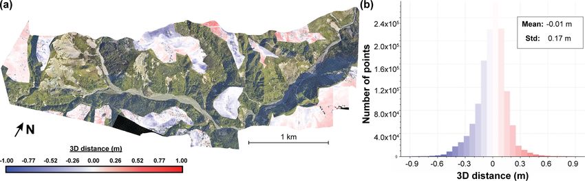
1020                                                       T. G. Bernard et al.: Beyond 2D landslide inventories and their rollover

Figure 2. Analysis of two main parameters of the M3C2 algorithm: the normal scale D and the projection scale d. Panel (a) shows the ratio
between the normal scale and mean roughness for different normal scale values (circles, left y axis), and the fraction of the pre-earthquake
core points for which the normal scale is 25 times larger than the local roughness (squares, right y axis). The dashed line highlights the
percentage of points with ζ >25 in the pre-EQ data for D = 10 m. Panel (b) shows the percentage of computed points with a confidence
interval of 95 % versus the projection scale d. The percentage of nonsignificant points is represented as well as the percentage of points
where the level of detection (LoD95 % ) was computed (i.e., with at least five points on each point cloud). The dashed line is set to 95 % and
highlights the threshold above which the projection scale is large enough to compute the LoD95 % on most of the core points.

Figure 3. (a, b, c) Workflow of the 3D point cloud differencing method for landslide detection and volume estimation with schematic
representations of the different steps: (a) the 3D measurement step with the shadow zone effect, where the red lines show the normal
orientation; (b) the vertical-M3C2 step; (c) segmentation by the connected component. The resulting sources and deposits are individual
point clouds illustrated in the figure using different colors.

to 20 cm for the pre-EQ survey, and is typically around 6 cm             first created by rasterizing the dataset with the largest point
for the post-EQ survey, with one pair of overlapping flight              density – here the post-EQ dataset – with a 1 m grid spac-
lines having a registration error of 12 cm. Hence, the inter-            ing. A vertical-M3C2 calculation is then performed, and the
nal registration quality of the pre-EQ dataset is significantly          mode of the resulting distribution is used to adjust the two
worse than the post-EQ dataset, a likely consequence of dif-             datasets by a vertical shift of 1.36 m. This approach is only
ferences in instrument precision and post-processing meth-               valid when the fraction of the surface affected by landsliding
ods.                                                                     is small. A subsequent 3D-M3C2 calculation is performed
   Second, the registration between the two surveys must be              to obtain a preliminary map of geomorphic change. At this
evaluated and generally improved. As delivered, the lidar                stage, a visual inspection of the pre-EQ and post-EQ or-
datasets have a vertical shift of between 1 and 2 m relative             thoimages and of the preliminary 3D-M3C2 distances allows
to each other. To correct for this shift, a grid of core points is       us to determine that there is no significant internal tectonic

Earth Surf. Dynam., 9, 1013–1044, 2021                                                      https://doi.org/10.5194/esurf-9-1013-2021
T. G. Bernard et al.: Beyond 2D landslide inventories and their rollover                                                        1021

displacement. We then manually define areas deemed sta-              ics and not to landslide deposits, are manually removed using
ble, 25 % of the studied area (Fig. 4a), to perform a cloud-         the post-EQ orthoimage. Along with the selection of the sta-
matching registration. The stable areas are defined as co-           ble areas, this is the only manual phase of the workflow.
herent surfaces (1) with a 3D-M3C2 distance smaller than
1 m, (2) where visual assessment of orthoimages suggested            3.4.3   Landslide source and deposit segmentation
no change had occurred, and (3) away from visible mass-
wasting processes and forested areas deduced from the anal-          Core points with negative and positive significant changes
ysis of the 3D-M3C2 distance map. Attention has been paid            are first separated into two distinct point clouds of sources
to select areas uniformly distributed in terms of location and       and deposits, respectively. A vertical-M3C2 is performed on
slopes in the studied region to maximize the registration qual-      each of these point clouds to estimate the volume of land-
ity.                                                                 slide sources and deposits (see Sect. 3.3.4). As for any 2D
   An iterative closest point (ICP) algorithm (Besl and              landslide inventory, a critical component of the workflow is
McKay, 1992) is then performed on the stable areas, and the          to segment each point cloud into individual landslide sources
obtained rigid transformation is applied to the entire post-         and areas. Segmenting complex patterns of erosion and de-
earthquake point cloud to align it with the pre-earthquake one       position in 3D, with a very wide range of sizes, is still a
(Table S2). The mean 3D-M3C2 distance on stable areas is             challenge. Here, for the sake of simplicity we use a clas-
−0.01 m, showing that there is almost no bias left in the reg-       sical clustering approach with a 3D connected component
istration, and the standard deviation of 3D-M3C2 distances           labeling algorithm (Lumia et al., 1983), available in Cloud-
is 0.17 m (Fig. 4b). At this stage, the two datasets are consid-     Compare (Fig. 3c). The point cloud is segmented into indi-
ered optimally registered for the stable areas but with an un-       vidual clusters based on two criteria: a minimum number of
known registration error reg. We propose defining reg as the         points or surface area (in our case), Amin , defining a clus-
maximum of the standard deviation of the intra-survey and            ter and a minimum distance, Dm , below which neighboring
inter-survey 3D-M3C2 distances in Eq. (2). In the ideal case         points, measured in a 3D Euclidean sense, belong to the same
of two very high-quality lidar datasets, reg would be equal to       cluster (Lumia et al., 1983). Amin was set to 20 m2 to be con-
the inter-survey registration error. In the studied case, the pre-   sistent with the area of the projection cylinder used to aver-
EQ intra-survey registration error is locally worse (0.2 m)          age the point cloud position in the M3C2 distance calcula-
than the inter-survey registration error (0.17 m). Thus, we set      tion, π (d/2)2 = 19.6 m2 with d = 5 m. Dm is an important
reg = 0.2 m, which is consistent with an estimate of reg that        parameter which, if an overly large value is chosen, will fa-
would be based on the combined lidar accuracy derived from           vor landslide amalgamation in identical clusters, and if an
GCP assuming complete correlation of errors (see Sect. 3.1).         overly small value is chosen, in relation to the core point
Consequently, and according to Eq. (2), with reg = 0.2 m,            spacing, may over-segment landslides. In any case, Dm must
our workflow cannot detect a 3D change that is smaller than          be larger than the core point spacing. As there is no objec-
0.40 m in the ideal case of a negligible roughness surface. At       tive way to a priori choose Dm , we explore various values
this stage, a 3D map of topographic change is available, but         and choose Dm = 2 m as an optimal value between landslide
the significant geomorphic changes and individual landslides         amalgamation and over-segmentation. The impact of Dm on
have not been isolated.                                              the statistical distribution of landslide sources is addressed in
                                                                     Sect. 5.
                                                                        We note that density-based clustering algorithms based on
3.4.2   Geomorphic change detection                                  DBSCAN (Density-Based Spatial Clustering of Applications
The registration error reg is then employed in a first applica-      with Noise; Ester et al., 1996) have been used for 3D rockfall
tion of 3D-M3C2, using the predetermined projection scale            inventory segmentation (e.g., Benjamin et al., 2020; Tonini
d = 5 m, to estimate the spatially variable LoD95 % according        and Abellan, 2014). These algorithms separate dense clus-
to Eq. (2). For core points in low-point-density areas, where a      ters of points, considered as areas of coherent topographic
confidence interval could not be estimated due to insufficient       change, from areas of low point density, considered as noise.
points, a second application of 3D-M3C2 is performed at a            As shown in the Supplement (Sect. S2), density-based clus-
larger projection scale d = 10 m. These core points generally        tering approaches do not yield a significantly better segmen-
correspond to ground points under canopy on steep slopes             tation than a connected component algorithm. However, they
and represent 9.5 % of the entire area and 12 % of steep             have several drawbacks ranging from slow computation time,
slopes prone to landsliding. Significant geomorphic changes          to less intuitive selection of parameters. Therefore, we have
at the 95 % confidence interval are then obtained by consid-         not used density-based clustering in our analysis.
ering core points with a 3D-M3C2 distance larger than the
LoD95 % . Significant geomorphic changes can be associated
with any geomorphic processes, including landsliding, but
also with fluvial erosion and deposition. Changes located in
the river bed, and likely specifically related to river dynam-

https://doi.org/10.5194/esurf-9-1013-2021                                               Earth Surf. Dynam., 9, 1013–1044, 2021
1022                                                   T. G. Bernard et al.: Beyond 2D landslide inventories and their rollover

Figure 4. (a) Map of 3D-M3C2 distances on stable areas and (b) the associated histogram. The map only displays 3D-M3C2 distance in the
areas chosen as stable for ICP registration and shows the post-earthquake orthoimage otherwise (Aerial Surveys, 2017).

3.4.4    Landslide area and volume estimation                        ventory after segmentation is provisional. The workflow has
                                                                     a classification step aiming at separating real landslides from
While 3D normal computation is optimal to detect geomor-             false detections using patch-based metrics. As the pre-EQ li-
phic changes, it is not suitable for volume estimation which         dar shows ground classification errors that would create false
requires the consideration of normals with parallel direc-           landslide sources (i.e., apparent negative change; Fig. 5a),
tions for a given landslide. Considering 3D normals can              and as we are specifically interested in the scaling relation-
lead to “shadow zones”, due to surface roughness, which              ships of sources, we focus on obtaining the best classification
would result in a biased volume estimate (Fig. 3a). There-           for sources and then simply use the proximity to the predicted
fore, distances and, in turn, volumes are computed by using          true landslides sources to select real deposits. To construct
a vertical-M3C2 on a grid of core points corresponding to the        the final landslide inventory, we apply the following steps:
significant changes (Fig. 3b). As the core points are regularly
spaced by 1 m, the landslide volume is simply the sum of               1. labeling of at least 60 % of the provisional source inven-
the vertical-M3C2 distances estimated from the individual-                tory as actual landslide sources and false detections;
ized landslides. While the distance uncertainty predicted by
the vertical-M3C2 could be used as the volume uncertainty,             2. evaluation of the classification potential of various fil-
it significantly overpredicts the true distance uncertainty due           tering metrics;
to nonoptimal normal orientation for the estimation of point           3. determination of the optimal filtering metrics based on
cloud roughness on steep slopes (i.e., the roughness is not the           a classification performance index;
detrended roughness). Thus, for each landslide source and
deposit, we compute the volume uncertainty from the sum                4. application of the optimal filtering metrics to classify
of the 3D-M3C2 uncertainty measured at each core point,                   the provisional landslide source inventory in predicted
not the vertical-M3C2 uncertainty. The volume uncertainty                 landslides and predicted false detections.
is specific to each landslide source and deposit and depends
                                                                        As the pre-EQ lidar data quality (point density and clas-
on the local surface properties, such as roughness, the num-
                                                                     sification) is significantly worse in forests than in forest-
ber of points considered and the global registration error,
                                                                     free areas, we carry out step 2 and 3 for provisional land-
but not on the volume itself. For each individual landslide
                                                                     slide sources located in forested and forest-free areas sepa-
source, the area A is obtained by computing the number of
                                                                     rately. Forest areas are defined based on the number of laser
core points inside the source region. This represents the verti-
                                                                     returns of the post-EQ dataset (Fig. S4). This corresponds
cally projected area which is also consistent with the existing
                                                                     to the number of targets a laser pulse has intercepted. For
literature based on 2D studies of landslide statistics. The dif-
                                                                     forest-free areas, this number is one, as the laser only hits
ference between planimetric area and true surface area (i.e.,
                                                                     the ground. However, in forested areas this number is ex-
measured parallel to the surface) is addressed in Sect. 5.
                                                                     pected to be greater than one, as tree elements create addi-
                                                                     tional echoes before the laser hits the ground. Thus, for each
3.5     Treatment of false detections                                core points, we calculate the average number of laser returns
                                                                     in a neighborhood of 2.5 m, to be consistent with the pro-
Owing to the simplified formulation of the LoD95 % (Eq. 2),          jection scale d, using the post-EQ lidar point cloud, which
it is possible for spatially correlated errors to create patches     has the best canopy penetration. We then consider that any
of statistically significant change that would appear after seg-     core point with an average number of laser returns equal to
mentation as false landslide detection (Fig. 5). Hence, the in-      or higher than two is in forested areas.

Earth Surf. Dynam., 9, 1013–1044, 2021                                                 https://doi.org/10.5194/esurf-9-1013-2021
T. G. Bernard et al.: Beyond 2D landslide inventories and their rollover 1023
Figure 5. Illustration of two types of labeled false detections. (a) A false detection located in a forest due to vegetation incorrectly classified
as ground in the pre-EQ point cloud. The false detection is overlaid on the post-EQ orthoimagery (Aerial Surveys, 2017). The apparent
negative topographic change creates a source. Note the limited penetration of the pre-EQ lidar in the dense evergreen forest that makes
ground classification extremely difficult. (b) A false detection due to pre-EQ intra-survey registration errors. Yellow points on the post-EQ
orthoimagery (Aerial Surveys, 2017) and the M3C2 distance field indicate patches of significant change that are a false detection. They
occur due to a complex combination of intra-line errors related to time-dependent attitude and position errors and intra-survey flight-line
registration error. Flight line 524 appears to be correctly registered to the post-EQ data, but flight line 217 is slightly misaligned, which
increases the likelihood of significant change detection.
3.5.1 Construction of a labeled source inventory debris flows, landslides or rockfalls, or (2) the presence
of scars.
The reference labeled source inventory is created with two
classes, actual landslide source and false detection, accord- 2. The structure of the two point clouds does not show high
ing to the following procedure. We first manually label all local points due to the misclassification of vegetation
of the provisional landslide sources with an area higher than (Fig. 5a).
200 m2 , as they are expected to correspond to the largest
3. The surrounding 3D-M3C2 field does not show a large
part of the total volume and are therefore critical. Provi-
constant value indicative of a locally incorrect registra-
sional landslide sources with A < 200 m2 are then divided
tion (Fig. 5b)
into 20 m2 area ranges. Following this, we choose to sample
and label 60 % of the provisional landslide sources located 4. The provisional source can be associated with at least
in each area range in order to be representative of the provi- one downstream provisional deposit within a radius of
sional inventory and avoid a size bias. Attention has been 30 m.
paid to ensuring spatially uniform and equally distributed
sampling between provisional landslide sources located in Not all criteria have to be met simultaneously. Uncertain
forested and forest-free areas. provisional landslide sources have been labeled as false de-
The labeling of actual landslide sources and false detec- tection. The resulting labeled inventory is then used as a ref-
tions is based on a visual inspection of the pre-EQ and erence to evaluate the filtering performance.
post-EQ orthophotos, of the pre-EQ and post-EQ lidar point
clouds, and of the 3D-M3C2 field and the provisional deposit 3.5.2 Definition of filtering metrics
inventory. We consider an actual landslide source according
to the following criteria: As false detections mainly emerge from the errors in the data
in relation to the amplitude of a real topographic change that
we aim to capture, we first choose to analyze three metrics
1. One of the following signs of mass movement is visible based on the 3D-M3C2 calculation: (1) the maximum 3D
on orthoimagery – (1) a drastic change in color between distance, (2) the mean LoD95 % and (3) the mean signal-to-
the pre-EQ and post-EQ orthophotos due to avalanches, noise ratio (SNR). We expect the maximum 3D distance to
https://doi.org/10.5194/esurf-9-1013-2021 Earth Surf. Dynam., 9, 1013–1044, 20211024 T. G. Bernard et al.: Beyond 2D landslide inventories and their rollover
discriminate between deep actual landslide sources and low- mum combination of two), we did not use machine learning
amplitude false detections arising from flight-line misalign- approaches to train the classifier.
ments and residual registration errors characteristic of false
detections in forest-free areas (Fig. 5b). As the LoD95 % is 3.6 Comparison with a manually mapped inventory
a direct measure of the quality of the data (point density and based on orthoimagery
roughness), classification errors of vegetation should be char-
acterized by a significantly higher mean LoD95 % than actual To estimate the potential in terms of landslide topographic
landslide sources. The SNR is defined as the ratio between change detection between the 3D-PcD method (3D-predicted
the 3D-M3C2 distance and the associated LoD95 % for each inventory) and a traditional approach, we created a second
core point. This measure can be used as a confidence metric inventory (2D inventory) by manually delineating landslide
for each source. sources based on a visual interpretation of the pre- and post-
We also choose to take advantage of the ability of the 3D EQ orthoimages, looking for texture change consistent with
differencing approach to detect deposit areas to analyze the landslide scars. The lidar data were not used in the process,
closest deposit distance (CDD). The CDD is defined for each and the map maker did not have a detailed knowledge of
provisional source as the closest downslope distance to a pro- the 3D-predicted inventory. Deposits were not mapped. The
visional deposit along the flow path using a D8 (determin- 2D and 3D landslide source inventories were then compared
istic eight-node) algorithm (Fairfield and Leymarie, 1991). in terms of the number of landslides and the intersection of
This distance is calculated from the post-EQ DEM with the mapped surfaces in planimetric view using GIS software. For
MATLAB-based TopoToolbox software (Schwanghart and source areas only detected by manual mapping, we define
Scherler, 2014). four classes: (1) areas located on deposit zones detected by
Metrics with the best potential are then tested to determine the 3D-PcD method, (2) areas under the LoD95 % , (3) areas
an optimal configuration of filtering metrics that best remove filtered by the minimum area of 20 m2 and (4) areas filtered
false detections while retaining the maximum number of ac- by the application of the optimal filtering metrics. For areas
tual landslide sources. The resulting predicted source inven- only detected by the 3D-PcD method, we distinguish land-
tory is then employed to filter the provisional landslide de- slide areas located in three land cover classes: (1) forest,
posit inventory by selecting the deposits that are connected (2) bare-rock and (3) other land covers. Forested areas are
to an upstream predicted landslide source along the flow path defined according to the number of returns of the post-EQ
using TopoToolbox (Schwanghart and Scherler, 2014). The lidar (see Sect. 3.5), whereas bare rocks are delineated man-
resulting inventory is called the predicted deposit inventory. ually on the orthoimages. We finally analyze the proportion
of areas only detected with the 3D-PcD approach that are
connected to a landslide source in the 2D inventory.
3.5.3 Definition of a classification performance index
To estimate the performance of the filtering metrics, we use 4 Results
the balanced accuracy (BA; Brodersen et al., 2010; Brodu
and Lague, 2012), defined as the average accuracy obtained 4.1 Geomorphic change and results of the
on the two predicted classes: segmentation
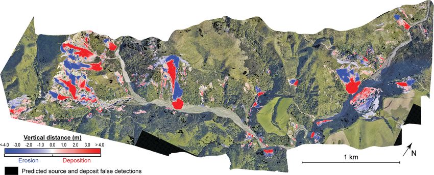
1 The map of 3D-M3C2 distances (Fig. 6a) prior to statisti-
BA = (TPrate + TNrate ), (3) cally significant change analysis and segmentation provides
2
a rare insight into topographic changes following a large
where, in our case, TPrate represents the percentage of cor- earthquake. At first order, it highlights areas of coherent pat-
rectly classified actual sources compared with the total la- terns of large (3D-M3C2 > 4 m) erosion (i.e., negative 3D
beled actual sources. Similarly, TNrate represents the percent- distances) and deposition (i.e., positive 3D distances) located
age of correctly classified false detections compared with the on hillslopes and corresponding to major landslides. Simple
total labeled false detections. This index not only reflects the configurations with one major source area and a single de-
overall performance of the filtering but also how TPrate and posit area can easily be recognized. A more complex pattern
TNrate are balanced, thereby avoiding a biased representation of intertwined landslides and rockfalls occurs on a bare-rock
of the filtering accuracy by the most frequent class. High val- surface in the western part of the study area, with a large va-
ues of BA are obtained when TPrate and TNrate are high and riety of source sizes and apparent aggregation of deposits.
balanced. The BA can be estimated based on the number, the Most of the deposits are located on hillslopes; however, the
area or the volume of the predicted landslides (BAn , BAa and deposits of three large landslides have reached the river and
BAv , respectively), and we define BAn,a,v as the mean of the altered its geometry. At second order, a variety of patches of
BAn , BAa and BAv . By exploring a range of values for each smaller amplitude (< 2 m) are visible on hillslopes. Erosion–
filtering metric, we find the value that maximizes BA. Given deposition patterns in relation to fluvial activity can be doc-
the limited number of metrics that we use at once (a maxi- umented on the river bed. The flight-line mismatch, iden-
Earth Surf. Dynam., 9, 1013–1044, 2021 https://doi.org/10.5194/esurf-9-1013-2021You can also read