Brief communication: Evaluation and inter-comparisons of Qinghai-Tibet Plateau permafrost maps based on a new inventory of field evidence - The ...
←
→
Page content transcription
If your browser does not render page correctly, please read the page content below
The Cryosphere, 13, 511–519, 2019
https://doi.org/10.5194/tc-13-511-2019
© Author(s) 2019. This work is distributed under
the Creative Commons Attribution 4.0 License.

Brief communication: Evaluation and inter-comparisons of
Qinghai–Tibet Plateau permafrost maps based on a new
inventory of field evidence
Bin Cao1,2 , Tingjun Zhang1 , Qingbai Wu3 , Yu Sheng3 , Lin Zhao4 , and Defu Zou5
1 Key  Laboratory of Western China’s Environmental Systems (Ministry of Education), College of Earth and Environmental
Sciences, Lanzhou University, Lanzhou 730000, China
2 Department of Geography & Environmental Studies, Carleton University, Ottawa K1S 5B6, Canada
3 State Key Laboratory of Frozen Soil Engineering, Cold and Arid Regions Environmental and Engineering Research

Institute, Chinese Academy of Sciences, Lanzhou 730000, China
4 School of Geographical Sciences, Nanjing University of Information Science and Technology, Nanjing 210044, China
5 Cryosphere Research Station on the Qinghai–Tibet Plateau, State Key Laboratory of Cryospheric Science, Cold and Arid

Regions Environmental and Engineering Research Institute, Chinese Academy of Sciences, Lanzhou 730000, China

Correspondence: Tingjun Zhang (tjzhang@lzu.edu.cn)

Received: 31 August 2018 – Discussion started: 18 September 2018
Revised: 31 January 2019 – Accepted: 1 February 2019 – Published: 12 February 2019

Abstract. Many maps have been produced to estimate per-          due to high ground temperature ( > −2 ◦ C) (Wu and Zhang,
mafrost distribution over the Qinghai–Tibet Plateau (QTP),       2008), and its distribution has strong influences on hydrolog-
but the errors and biases among them are poorly understood       ical processes (e.g. Cheng and Jin, 2013; Zhang et al., 2018),
due to limited field evidence. Here we evaluate and inter-       biogeochemical processes (e.g. Mu et al., 2017), and human
compare the results of six different QTP permafrost maps         systems (e.g. Wu et al., 2016).
with a new inventory of permafrost presence or absence com-         Many approaches have been used to produce permafrost
prising 1475 field sites compiled from various sources. Based    distribution and ground ice condition maps at different scales
on the in situ measurements, our evaluation results showed a     over the QTP (Ran et al., 2012). Typically, these maps clas-
wide range of map performance, with Cohen’s kappa coef-          sify frozen ground into permafrost and seasonally frozen
ficient from 0.21 to 0.58 and an overall accuracy between        ground, and information on the extent, such as the areal abun-
about 55 % and 83 %. The low agreement in areas near the         dance, of permafrost is available for some of them (Ran
boundary between permafrost and non-permafrost and in            et al., 2012). These maps significantly improved the un-
spatially highly variable landscapes highlights the need for     derstanding of permafrost distribution over the QTP. How-
improved mapping methods that consider more controlling          ever, limited in situ measurements and the different classi-
factors at both medium–large and local scales.                   fication systems and compilation approaches used make it
                                                                 challenging to compare maps directly. With the availability
                                                                 of high-resolution spatial datasets (e.g. surface air temper-
                                                                 ature and land surface temperature), several empirical and
1   Introduction                                                 (semi-)physical models have been applied in permafrost dis-
                                                                 tribution simulations at fine scales (e.g. Nan et al., 2013;
Permafrost is one of the major components of the cryosphere      Zhao et al., 2017; Zou et al., 2017; Wu et al., 2018). The
due to its large spatial extent. The Qinghai–Tibet Plateau       QTP has also been included in hemispheric or global maps
(QTP), also known as the Third Pole, has the largest extent of   including the Circum-Arctic Map of Permafrost and Ground-
permafrost in the low–middle latitudes. Permafrost over the      Ice Conditions produced by the International Permafrost As-
QTP was reported to be sensitive to climate change mainly        sociation (denoted as the IPA map) (Brown et al., 1997) and

Published by Copernicus Publications on behalf of the European Geosciences Union.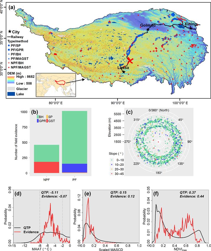
512                                                                    B. Cao et al.: Permafrost map evaluation over the QTP

the global permafrost zonation index (PZI) map (denoted as           lent coarse soil and low soil moisture content. The max-
the PZIglobal map) derived by Gruber (2012).                         imum thermal offset under natural conditions reported for
   Despite the increasing efforts in mapping QTP permafrost,         the QTP is 0.79 ◦ C (denoted as the maximum thermal off-
the maps have not been evaluated and inter-compared with             set, TOmax ) (Wu et al., 2002, 2010; Lin et al., 2015). In
the large amount of evidence of permafrost presence or ab-           this study, sites with MAGST+TOmax 6 0 ◦ C are considered
sence. These data have been collected since the 2000s and            to be permafrost sites. The reversed thermal offset reported
represent a number of different field techniques including           on the QTP was not considered here because thermal offset
ground temperature measurements, soil pits, and geophysics.          measurements are not available for all sites, and the influ-
A new inventory of this field evidence provides an oppor-            ence of the reversed thermal offset is expected to be mini-
tunity to improve the evaluation of the existing permafrost          mal due to its small magnitude (the value was reported as
maps. This is an important step in describing the current body       −0.07 ◦ C by Lin et al., 2015). GPR data are from Cao et al.
of knowledge on permafrost mapping performance as well as            (2017b) and were measured in 2014 between late September
identifying any possible bias. It is also critical for identifying   and November using 100 and 200 MHz antennas. The GPR
priorities when updating these maps in the future. Addition-         survey depth is from about 0.8 to nearly 5 m depending on
ally, an improved evaluation is a useful guide to selecting a        the active layer thickness. The data were carefully processed
map to use for permafrost and related studies, such as set-          by removing opaque reflections and evaluated using direct
ting boundary conditions for eco-hydrological model sim-             measurements. The ability of GPR data to detect permafrost
ulations. Climate change and increasing infrastructure con-          relies on the strong dielectric contrast between liquid water
struction on permafrost add both environmental and engi-             and ice (Moorman et al., 2003). Consequently, it is more dif-
neering relevance to investigating permafrost distribution and       ficult to discern the presence of permafrost in areas with low
increase the importance of evaluating and comparing existing         soil moisture content because it weakens this contrast (Cao
permafrost maps.                                                     et al., 2017b). For this reason, the GPR data were only con-
   In this study, we aim to                                          sidered to indicate the presence of permafrost if an active
                                                                     layer thickness could be established.
    1. provide the first inventory of evidence of permafrost            In order to apply the permafrost presence or absence in-
       presence or absence for the QTP; and                          ventory more broadly, the degree of confidence in the data is
                                                                     estimated and provided in the inventory and in Table 1, al-
    2. use the inventory to evaluate and inter-compare existing
                                                                     though it is not used in this study. BH and SP provide direct
       permafrost maps of the QTP.
                                                                     evidence of permafrost presence or absence based on MGT
                                                                     and/or ground ice observations, and hence have high con-
2     Data and methods                                               fidence (Cremonese et al., 2011). The data confidence de-
                                                                     rived from MAGST is classified based on temperature and
2.1    Inventory of permafrost presence or absence                   the length of the observation period. The evaluated GPR sur-
       evidence                                                      vey result was considered to have medium confidence.

Four methods were used to acquire evidence of per-                   2.2   Topographical and climatological properties of the
mafrost presence or absence: borehole temperature (BH), soil               inventory sites
pit (SP), ground surface temperature (GST), and ground-
penetrating radar (GPR) surveys (Fig. 1, Table 1). In this           The slope and aspect for the inventory sites were derived
study, we used the mean ground temperatures (MGTs) mea-              from a digital elevation model (DEM) with 3 arcsec spatial
sured from the boreholes, the depths of which vary from a            resolution, which is aggregated from the Global Digital Ele-
few metres to about 20 m depending on the depth of zero              vation Model Version 2 (GDEM2) by averaging to avoid the
annual amplitude and borehole depth, to identify permafrost          noise in the original dataset (Cao et al., 2017a). The ther-
presence or absence. At SP sites, the presence of ground ice         mal state and spatial distribution of permafrost result from
was used to indicate permafrost presence. However, due to            the long-term interaction of the climate and subsurface. Ad-
the prevalence of coarse soil, there are only six SP sites and       ditionally, vegetation and snow cover play important roles in
the depths range from less than 1 to about 2.5 m. Thermal            permafrost distribution by influencing the energy exchange
offset, here defined as the mean annual temperature at the           between the atmosphere and the ground surface (Norman
top of permafrost (TTOP) minus the mean annual ground                et al., 1995; Zhang, 2005). In this study, three climate vari-
surface temperature (MAGST) at a depth of 0.05 or 0.1 m,             ables were selected to test the representativeness of the inven-
was used to estimate permafrost presence or absence for sites        tory for permafrost map evaluation: mean annual air temper-
with only GST available. Although it is spatially variable           ature (MAAT), mean annual snow cover days (MASCD), and
depending on soil and temperature conditions, the magni-             the annual maximum normalized difference vegetation index
tude of the thermal offset is small on the QTP compared              (NDVImax ). The MAAT was obtained from Gruber (2012).
with northern, high-latitude environments due to the preva-          It has a spatial resolution of 1 km and represents the refer-

The Cryosphere, 13, 511–519, 2019                                                         www.the-cryosphere.net/13/511/2019/
B. Cao et al.: Permafrost map evaluation over the QTP 513 Figure 1. (a) The location of the QTP, and the distribution of evidence of in situ permafrost presence (PF) or absence (NPF) over the QTP, superimposed on the background of the digital elevation model (DEM) with a spatial resolution of 30 arcsec. (b) Number of field evidence located in NPF and PF regions. SP means soil pit, GPR refers to ground-penetrating radar, BH stands field evidence measured by borehole drilling, and MAGST is the mean annual ground surface temperature. (c) Distribution of field evidence in terms of elevation (radius), slope (coloured), and aspect (0/360◦ represents north). Distributions of (d) mean annual air temperature (MAAT), (e) scaled mean annual snow cover days (MASCD), and (f) annual maximum NDVI (NDVImax ) for field evidence (red line) compared to the entire QTP (black line). Numbers in (d), (e), and (f) are mean values. Only the sites with MAAT < 0 ◦ C, which is the precondition for permafrost presence, are present in (d). ence period spanning 1961–1990. The MASCD, with a spa- year between 2001 and 2017 to represent the approximate tial resolution of about 500 m, was derived from a daily snow amount of vegetation and then aggregated to a median value cover product developed by Wang et al. (2015) based on for the entire period to avoid sensitivity to extreme values. MODIS products (MOD10A1 and MYD10A1). To improve These climate variables were extracted for field site locations the comparison of MASCD, it was scaled to values between based on nearest-neighbour interpolation. The outline of the 0 and 1 by dividing the total days of a given year, and the QTP is from Zhang et al. (2002); glacier outlines are from mean MASCD during 2003–2010 was produced as a predic- Liu et al. (2015), representing conditions in 2010; and lake tor. The annual maximum NDVI is from the MODIS/Terra data are provided by the Third Pole Environment Database. 16-day Vegetation Index product (MOD13Q1, v006) which has a spatial resolution of 250 m. It was computed for each www.the-cryosphere.net/13/511/2019/ The Cryosphere, 13, 511–519, 2019
514                                                                                          B. Cao et al.: Permafrost map evaluation over the QTP

Table 1. Classification algorithm of evidence of in situ permafrost presence or absence from various methods.

        Method        Indicator                                                      Survey depth                            Permafrost        Confidence degree
        BH            MGT 6 0 ◦ C                                                    A few metres to about 20 m              presence          high
        SP            ground ice presence                                            about 1.0–2.5 m                         presence          high
        GST           MAGST 6 − 2 ◦ C & observations > 3                             0.05 or 0.1 m                           presence          medium
                      MAGST 6 − 2 ◦ C & observations < 3                                                                     presence          low
                      MAGST > −2 ◦ C & MAGST + TOmax 6 0 ◦ C                                                                 presence          low
                      MAGST < 0 ◦ C & MAGST + TOmax > 0 ◦ C                                                                  ambiguous         –
                      MAGST > 0 ◦ C                                                                                          absence           medium
        GPR           active layer thickness could be estimated                      about 0.80–5.0 m                        presence          medium
      BH is the borehole temperature, SP is the soil pit, GST is the ground surface temperature, GPR is the ground-penetrating radar, MGT is the mean ground temperature,
      and MAGST is the mean annual ground surface temperature. TOmax , the maximum thermal offset under natural conditions reported for the QTP, is 0.79 ◦ C.
      “Ambiguous” means the data are not sufficient to determine permafrost conditions and are not included in the inventory.

2.3   Existing maps over the QTP                                                           introduced two end-member cases for either cold (conser-
                                                                                           vative or more permafrost) or warm (non-conservative or
                                                                                           less permafrost) conditions, into the PZIglobal map to allow
Table 2 gives a summary of the most widely used and re-                                    the propagation of uncertainty caused by input datasets and
cently developed permafrost maps over the QTP. In general,                                 model suitability. The three cases or maps, denoted as the
permafrost maps over the QTP could be classified as (i) cat-                               PZInorm , PZIwarm , and PZIcold maps, differ in the parame-
egorical, using categorical classification with different per-                             ters used. Compared to the normal case, the cold and warm
mafrost categories (e.g. continuous, discontinuous, sporadic,                              variants are derived by shifting PZI and MAAT at the respec-
and island permafrost) or (ii) continuous, using a continuous                              tive limit by ±5 % and ±0.5 ◦ C, respectively. The PZIglobal
probability or index with a range of [0.01–1] to represent the                             map was partly evaluated for the QTP using rock glaciers,
proportion of an area that is underlain by permafrost. The IPA                             considered as indicators of permafrost conditions, based on
map, which may be the most widely used categorical map,                                    remote sensing imagery (Schmid et al., 2015). However, rock
was compiled by assembling all readily available data on                                   glaciers are absent in much of the QTP due to very low pre-
the characteristics and distribution of permafrost (Ran et al.,                            cipitation (Gruber et al., 2017).
2012). The IPA map uses the “permafrost zone” to describe
spatial patterns of permafrost, and the areas are divided into                             2.4    Statistics and evaluation of permafrost distribution
five categories based on the proportion of the ground un-                                         maps
derlain by permafrost: continuous (> 90 %), discontinuous
(50 %–90 %), sporadic (10 %–50 %), island (0 %–10 %), and                                  In order to compare maps, it is important to understand the
absent (0 %). The most recent efforts were made by Zou et al.                              difference between the extent of permafrost regions and the
(2017) using the TTOP model (denoted as the QTPTTOP map)                                   permafrost area. The permafrost area refers to the quantified
forced by a calibrated (using station data) land surface tem-                              extent of the area within a domain that is completely under-
perature (or freezing and thawing indices) considering soil                                lain by permafrost, whereas permafrost regions are categori-
properties and by Wu et al. (2018) based on the Noah land                                  cal areas within a domain that are defined by the percent of
surface model (denoted as the QTPNoah map) as well as grid-                                land area underlain by permafrost. For example, extensive
ded meteorological datasets, including surface air tempera-                                discontinuous permafrost is a region where, by definition,
ture, radiation, and precipitation. Although these two cate-                               50 % to 90 % of the land area is underlain by permafrost.
gorical maps are expected to be superior because they use the                              In this discontinuous permafrost region of a known area, the
latest measurements and advanced methods, they were eval-                                  area actually underlain by permafrost is the permafrost area
uated using limited and narrow distributed data (∼ 200 sites                               (Zhang et al., 2000).
for the QTPTTOP map and 56 sites for the QTPNoah map).                                        To conduct the map evaluations compared to measure-
The PZIglobal map, which gives a continuous index value                                    ments with binary information (presence or absence), it was
for permafrost distribution, is derived through a heuristic–                               necessary to develop classification aggregations for the exist-
empirical relationship with mean annual air temperature                                    ing maps. We argue that although the aggregation presented
(MAAT) based on generalized linear models (Gruber, 2012).                                  here simplifies the information available in these maps and
The model parameters are established largely based on the                                  may introduce uncertainty for further analyses, it is neces-
boundaries of continuous (PZI = 0.9 for MAAT = −8.0 ◦ C)                                   sary in order to conduct inter-comparisons among them. For
and island (PZI = 0.1 for MAAT = −1.5 ◦ C) permafrost in                                   the IPA map, we consider the continuous and discontinu-
the IPA map and do not use field observations. Gruber (2012)                               ous permafrost zones to correspond to permafrost presence

The Cryosphere, 13, 511–519, 2019                                                                                       www.the-cryosphere.net/13/511/2019/
B. Cao et al.: Permafrost map evaluation over the QTP 515
Table 2. Summary and evaluation of existing permafrost maps over the Qinghai–Tibet Plateau.
Name IPA QTPTTOP QTPNoah PZInorm PZIwarm PZIcold
Year 1997 2017 2018 2012 2012 2012
Method – semi-physical model physical model heuristic GLM heuristic GLM heuristic GLM
Classification criteria categorical categorical categorical continuous continuous continuous
Scale 1 : 10 000 000 ∼ 1 km 0.1◦ (∼ 10 km) ∼ 1 km ∼ 1 km ∼ 1 km
PCCPF (%) 46.6 93.9 96.4 76.6 35.3 94.3
PCCNPF (%) 79.8 58.6 45.9 82.6 98.5 54.0
PCCtol (%) 57.0 82.8 80.7 78.5 55.1 81.7
κ 0.21 0.58 0.52 0.56 0.36 0.55
PF region (106 km2 ) 1.63 – – 1.68 1.42 1.84
PF area (106 km2 ) – 1.06 ± 0.09 1.13 1.00 0.76 1.25
Reference Brown et al. (1997) Zou et al. (2017) Wu et al. (2018) Gruber (2012) Gruber (2012) Gruber (2012)
Evaluations are conducted using 1475 in situ measurements of permafrost presence or absence. GLM is the generalized linear model, and PF is permafrost. Norm (normal), warm, and cold
mean different cases and assumptions of parameters for permafrost distribution simulations in the PZIglobal map; details are given in Table 1 of Gruber (2012). The continuous
classification criteria mean the permafrost spatial patterns are compiled or present as a continuous value with a range of [0.01–1], e.g. the permafrost zonation index in the PZI maps.
and the other zones (sporadic permafrost, island permafrost, two categories (presence and absence), Cohen’s kappa co-
and non-permafrost) to correspond to permafrost absence efficient (κ), which measures inter-rater agreement for cat-
by using the proportion of ground underlain by permafrost egorical items (Landis and Koch, 1977), was used for map
of 50 % as a threshold. This is consistent with the thresh- evaluation:
old of the PZI map described below. For the QTPTTOP and po − pe
QTPNoah maps, the permafrost distribution was derived us- κ= , (4)
1 − pe
ing simulated mean annual ground temperature (thermally
defined). In these maps, areas are classified into three types: where pe and po are the probability of random agreement
permafrost, seasonally frozen ground, and unfrozen ground. and disagreement, respectively, and can be calculated as
Here, we merge the areas of seasonally frozen ground and
unfrozen ground to yield areas of permafrost absence. For (PFT + PFF ) × (PFT + NPFF )
pe = (5)
the PZI maps, specified thresholds are required for both the (PFT + PFF + NPFF + NPFT )2
extent of permafrost region and permafrost area. Following (NPFF + NPFT ) × (PFF + NPFT )
po = . (6)
Gruber (2012), only the areas with PZI ≥ 0.01 were selected (PFT + PFF + NPFF + NPFT )2
for further analysis, permafrost regions were defined as re-
Cohen’s kappa coefficient results are interpreted to mean
gions where PZI ≥ 0.1, and permafrost area was calculated
excellent agreement for κ > 0.8, substantial agreement for
as PZI multiplied by the pixel area. A value of 0.5 was used
0.6 6 κ < 0.8, moderate agreement for 0.4 6 κ < 0.6, slight
as the threshold of permafrost presence and absence (Boeckli
agreement for 0.2 6 κ < 0.4, and poor agreement for κ <
et al., 2012; Azócar et al., 2017).
0.2.
Maps were evaluated based on field evidence to produce
accuracy measurements as follows (Wang et al., 2015):
3 Results and discussion
PFT
PCCPF = × 100 % (1)
PFT + PFF 3.1 Evidence of permafrost presence or absence
NPFT
PCCNPF = × 100 % (2) There are a total of 1475 sites of permafrost presence or ab-
NPFT + NPFF
PFT + NPFT sence contained in the inventory acquired using BH, SP, GST,
PCCtol = × 100 %, (3) and GPR methods (Fig. 1). Among these, 1141 (77.4 %)
PFT + PFF + NPFT + NPFF
sites were measured by BH, 184 (12.5 %) sites by GST, 144
where PFT is the number of permafrost sites correctly classi- (9.8 %) sites by GPR, and 6 (0.4 %) sites by SP (Fig. 1b).
fied as permafrost, and PFF is the number of permafrost sites There are 1012 (68.6 %) sites of permafrost presence and 463
incorrectly classified as non-permafrost. Similarly, NPFT is (31.4 %) sites of permafrost absence. The data cover a large
the number of permafrost-absent sites correctly classified as area of the QTP (latitude: 27.73–38.96◦ N, longitude: 75.06–
non-permafrost, and NPFF is the number of incorrectly clas- 103.57◦ E) and a wide elevation range from about 1600 to
sified non-permafrost sites. PCC is the percentage of sites above 5200 m. However, the majority of sites (93.2 %) are lo-
correctly classified, and the subscripts PF, NPF, and tol indi- cated between 3500 and 5000 m. The inventory has an even
cate permafrost, non-permafrost, and total sites, respectively. distribution of aspects, with 27.3 % on the east slope, 27.9 %
To avoid the impact of unequal sample sizes in each of the on the south slope, 22.0 % on the west slope, and 22.6 % on
www.the-cryosphere.net/13/511/2019/ The Cryosphere, 13, 511–519, 2019516 B. Cao et al.: Permafrost map evaluation over the QTP
the north slope. Most of the sites (96.1 %) have slope angles nored. In this case, land surface temperature is underesti-
less than 20◦ (Fig. 1c). mated in high or dense vegetation areas because it comes
Figure 1d, e, and f compare the distribution of three from the top of the vegetation canopy, and it is overestimated
climate variables between the field sites and the entire in snow-covered areas where the cooling effects of snow are
QTP. The 1475 field sites have a narrower MAAT range not considered. As a consequence, permafrost is likely over-
(−10.5 to 15.7 ◦ C, with 25th percentile = −6.0 ◦ C and estimated in areas of high or dense vegetation and underes-
75th percentile = −3.8 ◦ C) compared to the entire QTP, timated in regularly snow-covered areas. While the QTPNoah
which has a MAAT between −25.6 and 22.1 ◦ C (25th per- map performed slightly better (2.5 % higher) for permafrost
centile = −6.6 ◦ C and 75th percentile = −0.41 ◦ C), and only area than the QTPTTOP map, it suffered from considerable
1.5 % sites located in the area with MAAT < −8 ◦ C. How- underestimation of the non-permafrost area (12.7 % lower for
ever, the data (88.2 %) were mostly found in the most sensi- PCCNPF ). Although the QTPNoah map was derived using a
tive MAAT range (from −8 to −2 ◦ C) for permafrost pres- coupled land surface model (Noah), the poorer performance,
ence or absence (Gruber, 2012; Cao et al., 2018). There is especially for the non-permafrost area (PCCNPF = 49.5 %),
a slight bias in the scaled MASCD coverage. Few measure- is likely caused by the coarse-scale forcing dataset (0.1◦ res-
ments (7.5 %) were located in areas of high scaled MASCD olution or ∼ 10 km) and by the uncertainty in the soil tex-
(> 0.20) due to the associated harsh climate and inconve- ture dataset (Chen et al., 2011; Yang et al., 2010). It is not
nient access. The NDVImax at field evidence sites has a wide surprising that the IPA map has slight agreement (κ = 0.21)
coverage for the QTP, with a range of 0.05–0.88. The higher because fewer observations were compiled and the methods
mean NDVImax for field sites (0.44 at the sample sites and used were more suitable for high latitudes (Ran et al., 2012).
0.37 for the QTP) is due to the fact that measurements were For the PZI map, the PZInorm and PZIcold maps were found
normally collected in flat areas with relatively dense vegeta- to be in moderate agreement (κ = 0.56 for the PZInorm map
tion cover. These results suggest that the evaluation presented and 0.55 for the PZIcold map) with in situ measurements,
in this study is representative of most of the QTP but may and they performed slightly worse than the QTPTTOP map.
have more uncertainty in steep and regularly snow-covered The poor performance of the PZIwarm map and underesti-
regions. mation of the PZInorm map indicated that permafrost over
the QTP is more prevalent than most of the other regions,
3.2 Evaluation and comparison of existing maps even though the climate conditions, especially the MAAT,
are similar. This is likely because of the high soil thermal
The new inventory was used to evaluate existing permafrost conductivity due to coarse soil and the cooling effects of
maps derived with different methods (Table 2). In general, minimal snow (Zhang, 2005). Large differences of the per-
these permafrost maps showed different performances, in- mafrost region (0.42 × 10⁶ km2 , or 25 % of the normal case)
cluding slight agreement for the IPA map, fair agreement for and area (0.49 × 10⁶ km2 , or 49 % of the normal case) were
the PZIwarm map, and moderate agreement for the QTPNoah , found for the three cases of the PZIglobal map, though the up-
PZInorm , PZIcold , and QTPTTOP maps, with a wide spread per and lower bounds only changed about 5 % for the PZI
of κ from 0.21 to 0.58. The high PCCPF together with low and ±0.5 ◦ C for the MAAT. The MAAT used in the PZIglobal
PCCNPF for the QTPNoah , PZIcold , and QTPTTOP maps in- map was statistically downscaled from reanalysis based on
dicate permafrost is overestimated by them, while the IPA, the lapse rate derived from NCEP upper-air (pressure level)
PZIwarm , and PZInorm maps underestimated the permafrost temperatures. The land surface influences on surface air tem-
over the QTP. Despite the small permafrost area bias for perature, such as cold air pooling, were ignored (Cao et al.,
the QTPTTOP and QTPNoah maps caused by different QTP 2017a). This is important as winter inversions are expected
boundaries, lake, and glacier datasets used, the range of the to be common due to the prevalent mountains over the QTP.
estimated permafrost region (1.42–1.84 × 10⁶ km2 , or 30 % In other words, permafrost may be underestimated in valleys
difference) and area (0.76–1.25 × 10⁶ km2 , or 64.4 % differ- due to the overestimated MAAT.
ence) is extremely large (Fig. 2). Spatially, the non-permafrost areas of the southeastern
Among the categorical maps, the QTPTTOP map achieved QTP are well represented in all maps, while misclassifica-
the best performance for permafrost distribution over the tion is prevalent in areas near the boundary between per-
QTP, with the highest κ (0.58, moderate agreement) and mafrost and non-permafrost and in spatially highly variable
PCCtol (82.8 %); however, caution should be taken when in- landscapes such as the sources of the Yellow River (Fig. 2).
terpolating the map. The QTPTTOP map was derived based This is because the permafrost spatial patterns in these ar-
on MODIS land surface temperature with temporal cover- eas are not only controlled by medium- to large-scale climate
age of 2000–2012 (Zou et al., 2017). Though the MODIS conditions (e.g. MAAT), which are described by the models
land surface temperature time-series gaps caused mainly by used, but are also strongly influenced by various local factors
clouds were filled using the Harmonic Analysis of Time Se- such as peat layers, thermokarst, soil moisture, and hydrolog-
ries (HANTS) algorithm (Prince et al., 1998), the surface ical processes. The IPA and PZIwarm maps showed a fit that
conditions, especially vegetation and snow cover, were ig- is only good in some areas (e.g. relatively colder areas for the
The Cryosphere, 13, 511–519, 2019 www.the-cryosphere.net/13/511/2019/B. Cao et al.: Permafrost map evaluation over the QTP 517
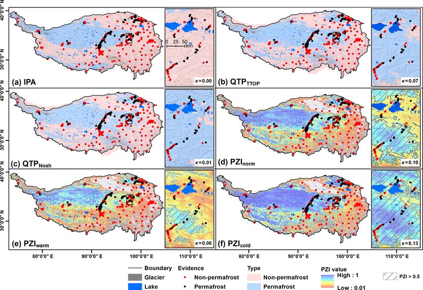
Figure 2. The permafrost classification results at in situ evidence sites shown on the (a) IPA, (b) QTPTTOP , (c) QTPNoah , (d) PZInorm ,
(e) PZIwarm , and (f) PZIcold maps. Cohen’s kappa coefficient (κ) was derived from the selected spatially highly variable landscapes (marked
by black box) with 106 evidence sites. All the maps are resampled to the unprojected grid of the SRTM30 DEM with a spatial resolution of
30 arcsec (∼ 1 km) to avoid map bias caused by different resolutions, geographic projection, and format. The boundary of QTP used in this
study is marked by the black line. Categorical classification is used for the QTPTTOP , QTPNoah , and IPA maps, while the continuous PZI
was present for the PZInorm , PZIwarm , and PZIcold maps. The blank parts in the PZI maps are areas with PZI < 0.01.
IPA map and southeastern area for the PZIwarm map) based with κ from 0.21 to 0.58 and an overall classification ac-
on the in situ measurements and may not represent the per- curacy of about 55 %–83 %. The misclassification is preva-
mafrost distribution patterns well for the other areas beyond lent in areas near the boundary between permafrost and non-
the measurements. permafrost and in spatially highly variable landscapes. This
highlights the need for improved mapping methods that con-
sider more controlling factors at both medium–large and lo-
4 Conclusions cal scales. The QTPTTOP map is recommended for represent-
ing permafrost distribution over the QTP based on our evalu-
We compiled an inventory of evidence of permafrost pres- ation. Additionally, the PZInorm and PZIcold maps are similar
ence or absence using 1475 field sites obtained based on di- to one another and are valuable alternatives for describing
verse methods over the QTP. With a wide coverage of to- a permafrost zonation index over the QTP. The inadequate
pography (e.g. elevation and slope aspect) and climate con- sampling in steep and regularly snow-covered areas is ex-
ditions (e.g. surface air temperature and snow cover), the in- pected to result in higher uncertainty for map evaluation and
ventory gives a representative baseline for site-specific per- requires further investigation using systematic samples.
mafrost occurrence.
The existing permafrost maps over the QTP were evalu-
ated and inter-compared using the inventory of ground-based
evidence, and they showed a wide range of performance,
www.the-cryosphere.net/13/511/2019/ The Cryosphere, 13, 511–519, 2019518 B. Cao et al.: Permafrost map evaluation over the QTP
Data availability. The inventory of permafrost presence or absence Cao, B., Gruber, S., and Zhang, T.: REDCAPP (v1.0): pa-
is partly available as a supplement, and the other evidence sites not rameterizing valley inversions in air temperature data down-
listed are available from the authors upon request. scaled from reanalyses, Geosci. Model Dev., 10, 2905–2923,
https://doi.org/10.5194/gmd-10-2905-2017, 2017a.
Cao, B., Gruber, S., Zhang, T., Li, L., Peng, X., Wang, K., Zheng, L.,
Supplement. The supplement related to this article is available Shao, W., and Guo, H.: Spatial variability of active layer thick-
online at: https://doi.org/10.5194/tc-13-511-2019-supplement. ness detected by ground-penetrating radar in the Qilian Moun-
tains, Western China, J. Geophys. Res.-Earth, 122, 574–591,
https://doi.org/10.1002/2016JF004018, 2017b.
Author contributions. BC carried out this study by organizing the Cao, B., Zhang, T., Peng, X., Mu, C., Wang, Q., Zheng, L.,
inventory of evidence of permafrost presence or absence, analysing Wang, K., and Zhong, X.: Thermal Characteristics and Recent
data, performing the simulations, and structuring as well as writing Changes of Permafrost in the Upper Reaches of the Heihe River
the paper. TZ guided the research. QW, YS, LZ, and DZ contributed Basin, Western China, J. Geophys. Res.-Atmos., 123, 7935–
to the organization of the dataset of permafrost presence or absence. 7949, https://doi.org/10.1029/2018JD028442, 2018.
Chen, Y., Yang, K., He, J., Qin, J., Shi, J., Du, J., and
He, Q.: Improving land surface temperature modeling for
dry land of China, J. Geophys. Res.-Atmos., 116, D20104,
Competing interests. The authors declare that they have no conflict
https://doi.org/10.1029/2011JD015921, 2011.
of interest.
Cheng, G. and Jin, H.: Permafrost and groundwater on the Qinghai-
Tibet Plateau and in northeast China, Hydrogeol. J., 21, 5–23,
https://doi.org/10.1007/s10040-012-0927-2, 2013.
Acknowledgements. The authors would like to thank the edi- Cremonese, E., Gruber, S., Phillips, M., Pogliotti, P., Boeckli, L.,
tor, Peter Morse, two anonymous reviewers, Stephan Gruber, Noetzli, J., Suter, C., Bodin, X., Crepaz, A., Kellerer-Pirklbauer,
and Kang Wang for their constructive suggestions. We thank A., Lang, K., Letey, S., Mair, V., Morra di Cella, U., Ravanel,
Nicholas Brown for improving the writing of an earlier version L., Scapozza, C., Seppi, R., and Zischg, A.: Brief Communi-
of the manuscript. We thank Zhuotong Nan and Xiaobo Wu for cation: “An inventory of permafrost evidence for the European
providing the QTPNoah map. This study was supported by the Alps”, The Cryosphere, 5, 651–657, https://doi.org/10.5194/tc-
Strategic Priority Research Program of Chinese Academy of 5-651-2011, 2011.
Sciences (XDA20100103, XDA20100313), the National Natural Gruber, S.: Derivation and analysis of a high-resolution estimate
Science Foundation of China (41871050, 41801028), and partly by of global permafrost zonation, The Cryosphere, 6, 221–233,
the Fundamental Research Funds for the Central Universities (lzu- https://doi.org/10.5194/tc-6-221-2012, 2012.
jbky_2016_281, 862863). We thank CMA (http://data.cma.cn/; last Gruber, S., Fleiner, R., Guegan, E., Panday, P., Schmid, M.-O.,
access: 6 February 2019) for providing the surface air and ground Stumm, D., Wester, P., Zhang, Y., and Zhao, L.: Review article:
surface temperatures. The GDEM2 dataset can be downloaded from Inferring permafrost and permafrost thaw in the mountains of
the United States Geological Survey (http://gdex.cr.usgs.gov/gdex/; the Hindu Kush Himalaya region, The Cryosphere, 11, 81–99,
last access: 6 February 2019). The NDVI datasets are derived https://doi.org/10.5194/tc-11-81-2017, 2017.
and processed in the Google Earth Engine. The glacier inventory Landis, J. R. and Koch, G. G.: The Measurement of Observer
is provided by the Environmental and Ecological Science Data Agreement for Categorical Data, Biometrics, 33, 159–174, 1977.
Center for West China (http://westdc.westgis.ac.cn/; last access: Lin, Z., Burn, C. R., Niu, F., Luo, J., Liu, M., and Yin, G.: The Ther-
6 February 2019), and the lake inventory is from the Third Pole mal Regime, including a Reversed Thermal Offset, of Arid Per-
Environment Database (http://www.tpedatabase.cn; last access: mafrost Sites with Variations in Vegetation Cover Density, Wu-
6 February 2019). daoliang Basin, Qinghai-Tibet Plateau, Permafrost Periglac., 26,
142–159, https://doi.org/10.1002/ppp.1840, 2015.
Edited by: Peter Morse Liu, S., Yao, X., Guo, W., Xu, J., Shangguan, D., Wei, J., Bao, W.,
Reviewed by: two anonymous referees and Wu, L.: The contemporary glaciers in China based on the
Second Chinese Glacier Inventory, Acta Geographica Sinica, 70,
3–16, 2015 (in Chinese with English abstract).
Moorman, B. J., Robinson, S. D., and Burgess, M. M.: Imaging
References periglacial conditions with ground-penetrating radar, Permafrost
Periglac., 14, 319–329, https://doi.org/10.1002/ppp.463, 2003.
Azócar, G. F., Brenning, A., and Bodin, X.: Permafrost distribution Mu, C., Zhang, T., Zhao, Q., Su, H., Wang, S., Cao, B., Peng,
modelling in the semi-arid Chilean Andes, The Cryosphere, 11, X., Wu, Q., and Wu, X.: Permafrost affects carbon exchange
877–890, https://doi.org/10.5194/tc-11-877-2017, 2017. and its response to experimental warming on the northern
Boeckli, L., Brenning, A., Gruber, S., and Noetzli, J.: Permafrost Qinghai-Tibetan Plateau, Agr. Forest Meteorol., 247, 252–259,
distribution in the European Alps: calculation and evaluation of https://doi.org/10.1016/j.agrformet.2017.08.009, 2017.
an index map and summary statistics, The Cryosphere, 6, 807– Nan, Z., Huang, P., and Zhao, L.: Permafrost distribu-
820, https://doi.org/10.5194/tc-6-807-2012, 2012. tion modeling and depth estimation in the Western
Brown, J., Ferrians Jr., O. J., Heginbottom, J. A., and Melnikov, Qinghai-Tibet Plateau, Acta Geographica Sinica, 68, 318,
E. S.: Circum-Arctic Map of Permafrost and Ground-ice Condi-
tions, 1997.
The Cryosphere, 13, 511–519, 2019 www.the-cryosphere.net/13/511/2019/B. Cao et al.: Permafrost map evaluation over the QTP 519 https://doi.org/10.11821/xb201303003, 2013 (in Chinese with Wu, X., Nan, Z., Zhao, S., Zhao, L., and Cheng, G.: Spa- English abstract). tial modeling of permafrost distribution and properties on Norman, J., Kustas, W., and Humes, K.: Source approach for esti- the Qinghai – Tibet Plateau, Permafrost Periglac., 29, 86–99, mating soil and vegetation energy fluxes in observations of di- https://doi.org/10.1002/ppp.1971, 2018. rectional radiometric surface temperature, Agr. Forest Meteorol., Yang, K., He, J., Tang, W., Qin, J., and Cheng, C. C.: 77, 263–293, 1995. On downward shortwave and longwave radiations over Prince, S., Goetz, S., Dubayah, R., Czajkowski, K., and Thaw- high altitude regions: Observation and modeling in the ley, M.: Inference of surface and air temperature, atmospheric Tibetan Plateau, Agr. Forest Meteorol., 150, 38–46, precipitable water and vapor pressure deficit using Advanced https://doi.org/10.1016/j.agrformet.2009.08.004, 2010. Very High-Resolution Radiometer satellite observations: com- Zhang, T.: Influence of the seasonal snow cover on the ground parison with field observations, J. Hydrol., 212–213, 230–249, thermal regime: An overview, Rev. Geophys., 43, RG4002, https://doi.org/10.1016/S0022-1694(98)00210-8, 1998. https://doi.org/10.1029/2004RG000157, 2005. Ran, Y., Li, X., Cheng, G., Zhang, T., Wu, Q., Jin, H., and Zhang, T., Heginbottom, J. A., Barry, R. G., and Brown, J.: Fur- Jin, R.: Distribution of Permafrost in China: An Overview of ther statistics on the distribution of permafrost and ground ice Existing Permafrost Maps, Permafrost Periglac., 23, 322–333, in the Northern Hemisphere, Polar Geography, 24, 126–131, https://doi.org/10.1002/ppp.1756, 2012. https://doi.org/10.1080/10889370009377692, 2000. Schmid, M.-O., Baral, P., Gruber, S., Shahi, S., Shrestha, T., Zhang, Y., Li, B., and Zheng, D.: A discussion on the boundary and Stumm, D., and Wester, P.: Assessment of permafrost distri- area of the Tibetan Plateau in China, Geogr. Res., 21, 1–8, 2002 bution maps in the Hindu Kush Himalayan region using rock (Chinese with English abstract). glaciers mapped in Google Earth, The Cryosphere, 9, 2089– Zhang, Y. L., Li, X., Cheng, G. D., Jin, H. J., Yang, D. W., 2099, https://doi.org/10.5194/tc-9-2089-2015, 2015. Flerchinger, G. N., Chang, X. L., Wang, X., and Liang, J.: In- Wang, W., Huang, X., Deng, J., Xie, H., and Liang, T.: Spatio- fluences of Topographic Shadows on the Thermal and Hydro- Temporal Change of Snow Cover and Its Response to Cli- logical Processes in a Cold Region Mountainous Watershed in mate over the Tibetan Plateau Based on an Improved Daily Northwest China, J. Adv. Model. Earth Sy., 10, 1439–1457, Cloud-Free Snow Cover Product, Remote Sensing, 7, 169–194, https://doi.org/10.1029/2017MS001264, 2018. https://doi.org/10.3390/rs70100169, 2015. Zhao, S., Nan, Z., Huang, Y., and Zhao, L.: The Application Wu, J., Sheng, Y., Wu, Q., and Wen, Z.: Processes and modes of and Evaluation of Simple Permafrost Distribution Models on permafrost degradation on the Qinghai-Tibet Plateau, Sci. China the Qinghai–Tibet Plateau, Permafrost Periglac., 28, 391–404, Ser. D, 53, 150–158, https://doi.org/10.1007/s11430-009-0198- https://doi.org/10.1002/ppp.1939, 2017. 5, 2010. Zou, D., Zhao, L., Sheng, Y., Chen, J., Hu, G., Wu, T., Wu, J., Xie, Wu, Q. and Zhang, T.: Recent permafrost warming on the C., Wu, X., Pang, Q., Wang, W., Du, E., Li, W., Liu, G., Li, J., Qinghai-Tibetan Plateau, J. Geophys. Res.-Atmos., 113, d13108, Qin, Y., Qiao, Y., Wang, Z., Shi, J., and Cheng, G.: A new map of https://doi.org/10.1029/2007JD009539, 2008. permafrost distribution on the Tibetan Plateau, The Cryosphere, Wu, Q., Zhu, Y., and Liu, Y.: Application of the Permafrost Table 11, 2527–2542, https://doi.org/10.5194/tc-11-2527-2017, 2017. Temperature and Thermal Offset Forecast Model in the Tibetan Plateau, Journal of Glaciology and Geocryology, 24, 614–617, 2002 (in Chinese with English abstract). Wu, Q., Zhang, Z., Gao, S., and Ma, W.: Thermal impacts of en- gineering activities and vegetation layer on permafrost in differ- ent alpine ecosystems of the Qinghai–Tibet Plateau, China, The Cryosphere, 10, 1695–1706, https://doi.org/10.5194/tc-10-1695- 2016, 2016. www.the-cryosphere.net/13/511/2019/ The Cryosphere, 13, 511–519, 2019
You can also read