Comparison of Research Findings on Avian Predation Impacts on Salmon Survival

Independent Scientific Advisory Board
 for the Northwest Power and Conservation Council,
 Columbia River Basin Indian Tribes,
 and National Marine Fisheries Service
 851 SW 6th Avenue, Suite 1100
 Portland, Oregon 97204

Comparison of Research Findings on Avian
 Predation Impacts on Salmon Survival

 Members

 Courtney Carothers
 John Epifanio
 Stanley Gregory
 Dana Infante
 William Jaeger
 Cynthia Jones
 Peter Moyle
 Thomas Quinn
 Kenneth Rose
 Carl Schwarz, Ad Hoc
 Thomas Turner
 Thomas Wainwright

 ISAB 2021-2
 April 23, 2021

Comparison of Research Findings on Avian
 Predation Impacts on Salmon Survival
Contents
Acknowledgements.........................................................................................................................iii
Executive Summary......................................................................................................................... 1
Background ..................................................................................................................................... 5
Summary of Haeseker et al (2020) and Payton et al. (2020) .......................................................... 5
 Study Domain and Data .......................................................................................................... 8
 Modeling Approaches ............................................................................................................. 9
Detailed Responses to the Assigned Questions............................................................................ 10
 1. Were the Haeseker et al. 2020 and Payton et al. 2020 analyses scientifically sound, and
 were the data used appropriate for addressing the question?........................................ 10
 2. Were the conclusions drawn by Haeseker et al. 2020 and Payton et al. 2020 analyses
 supported by their results? ............................................................................................... 17
 3. How do the modeling approaches of Haeseker et al. 2020 and Payton et al. 2020 differ,
 and do these analytical differences or other reasons account for the contrasts in their
 conclusions? ...................................................................................................................... 18
 4. Does the ISAB have recommendations to improve the analysis? .................................... 20
 5. What are the management implications of the results? .................................................. 22
Appendix A: Comparison of the predation equations used by Payton et al. (2020) and Haeseker
et al. (2020) ................................................................................................................................... 24
Appendix B: Effects of mortality associated with tagging and handling at dams ........................ 28
References .................................................................................................................................... 31

List of Figures
Figure 1. Estimated survival rates (±SE) for steelhead cohorts from the Snake River Basin, USA,
2000–2015 (Figure 4B in Haeseker et al. [2020]). ........................................................................ 12

 i

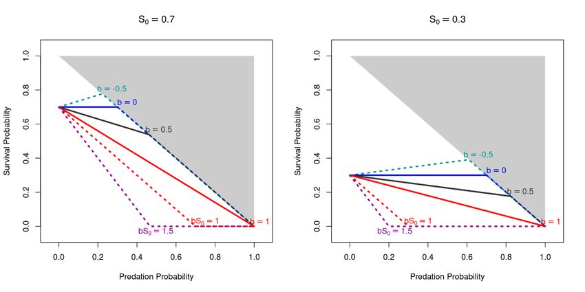
Figure 2. Weekly smolt‐to‐adult survival probabilities to Bonneville Dam for Snake River
steelhead as a function of Caspian tern predation probabilities in the Columbia River estuary in
each year from 2008 to 2016 and all years combined (Figure 8.S3 in Payton et al. 2021) .......... 13
Figure 3. Weekly probability estimates of steelhead smolt survival and Caspian Tern predation
along with the estimated annual relationships between survival and predation during out-
migration from Rock Island Dam to Bonneville Dam (Figure 3 in Payton et al. [2020]) .............. 15
Figure. 4. Estimated annual relationships between PIT-tagged steelhead smolt-to-adult survival
probabilities and Caspian Tern predation probabilities during smolt out-migration from Rock
Island Dam to the Pacific Ocean (Figure 4 in Payton et al. [2020]) .............................................. 16
Figure A.1. The full set of equations relating total survival to predation probabilities ............... 27
Figure B.1. SARs and raw tag recovery probability at Potholes Reservoir. .................................. 30

List of Tables
Table 1. Summary of the approach and methods of Haeseker et al (2020) and Payton et al.
(2020). ............................................................................................................................................. 7
Table A.1. Notation used in the survival-predation equations..................................................... 24

 ii

Acknowledgements
The ISAB gratefully acknowledges the many individuals who helped us complete this report.
The authors of both papers in this review provided excellent presentations, briefings, and
discussions of their research on the effects of avian predation on salmonids in the Columbia
River Basin. On February 19, 2021, Quinn Payton, Allen Evans, Ken Collis, Brad Watkins (Real
Time Research), Dan Roby (Oregon State University), and Nathan Hostetter (University of
Washington) presented a briefing to the ISAB on the analysis in Payton et al. (2020). On March
18, 2021, Steve Haeseker (U.S. Fish and Wildlife Service) presented and Jerry McCann, Gabe
Scheer, and Michele Dehart (Fish Passage Center) participated in a briefing to the ISAB on the
analysis in Haeseker et al. (2020). Both groups of researchers provided additional information
following their briefings to respond to ISAB questions and responded to inquiries from the ISAB
on technical accuracy on specific topics.
Tami Wilkerson and Maggie Willis of the Columbia River Inter-Tribal Fish Commission’s (CRITFC)
Columbia Basin Fish and Wildlife Library provided a Columbia River Basin Avian Predation
Bibliography.
The ISAB coordinator Erik Merrill and Ex Officio members Leslie Bach (Council), Zach Penney
(CRITFC), and Mike Ford (NOAA) helped organize our review, participated in briefings, provided
context, and commented on drafts.

 iii

Comparison of Research Findings on Avian
 Predation Impacts on Salmon Survival
Executive Summary
This ISAB report evaluates similarities and differences in data, analytical approaches,
conclusions, and management implications of two studies of avian predation on juvenile
steelhead in the Columbia River Basin. Both studies focused on determining whether the effects
of avian predation on overall survival were additive (meaning that the predation reduces
overall survival) or compensatory (meaning that other aspects of mortality offset or
compensate for predation). Haeseker et al. (2020) focused on bird predation in the Columbia
River estuary of migrating smolts from the Snake River Basin and its effect on survivorship
(return probability) of adults returning to Bonneville Dam. Haeseker et al. concluded that
mortality from avian predation was consistent with full compensation. In contrast, Payton et al.
(2020) estimated the effects of bird predation both in the river and in the estuary on Upper
Columbia Basin smolts at two life stages: from release at Rock Island Dam to Bonneville Dam as
smolts and from release to adult return to Bonneville Dam. Payton et al. concluded that
predation mortality was super-additive for smolts between Rock Island and Bonneville, and
partially additive from release to adult return to Bonneville Dam. Super-additive means causing
more smolts to die than the number of smolts estimated to be consumed by bird predators.
Sources for additional undetected mortality include deposition of PIT tags at locations other
than the colony, smolts being stolen by gulls, wounding or injury that results in mortality but
not capture by the predator, or consumption by birds that occupy areas other than the colonies
monitored for PIT tags.
Both studies relied on data from PIT-tagged smolts, detections of survivors at distinct points in
the hydrosystem, and mark-recapture models to estimate survival to a given life stage. Bird
predation was estimated from PIT-tags recovered from nesting colonies of Caspian terns and
double-crested cormorants at East Sand Island (in both studies) and bird colonies, including gull
species, located upstream of Bonneville Dam (in Payton et al. 2020). While the studies were
conducted in different basins and employed only partially overlapping time series, we
compared data and analyses from migration to adult return life stage to illuminate the nature
of conclusions and interpretations.
There are important differences in definitions and underlying models used to distinguish
additivity and compensation that could partly account for differences in conclusions between
the studies. Haeseker et al. (2020) used a correlation-based criterion to define and model
additivity and compensation, with full additivity or full compensation as strict theoretical limits

 1

of the analysis and partial additivity between these two limits. Payton et al. (2020) used a
regression-based definition and a model that also defines full additivity, full compensation, and
partial additivity, but also allowed for over-compensation and super-additivity as theoretical
possibilities that exceed the limits used by Haeseker et al. The analysis by Haeseker et al. de-
emphasized the distinction between partial and full additivity, instead interpreting a significant
negative correlation between survival and bird predation as indicating additivity (partial or full)
and an observed lack of correlation as consistent with full compensation.
The ISAB review responded to the following questions:
1. Were the Haeseker et al. 2020 and Payton et al. 2020 analyses scientifically sound, and
were the data used appropriate for addressing the question?
Compared with all other species and populations of salmonids in the Columbia Basin, steelhead
smolts are most vulnerable to avian predation (Roby et al. 2021). Accordingly, both studies
focused on steelhead. Both studies used reasonable approaches to assess mortality imposed on
steelhead from bird predation. Each analysis has a lengthy list of assumptions (some explicit,
others implicit, and discussed or not). Both studies attempted to test complicated hypotheses
with analysis of a complex dataset from tagging studies that were not designed specifically for
this purpose. Differences in annual mortality and tag recovery were identified across tagging
and release locations, but the ISAB found no evidence of significant bias in the context of
analysis across steelhead cohorts within years. Nonetheless, both studies demonstrate that
tagging data can be adapted for the important purpose of assessing effects of predators at
multiple sites in the Columbia Basin.
2. Were the conclusions drawn by Haeseker et al. 2020 and Payton et al. 2020 analyses
supported by their results?
In general, the conclusions of both studies are reasonably supported within the context of their
different model frameworks and definitions. Analytical differences between studies were
substantive, but these were not a result of variation in data quality or analysis. Differences in
conclusions, namely full compensation (Haeseker et al.) vs. partial additivity (Payton et al.) in
smolt-to-adult survival, could result from differences in statistical power between approaches,
differences in the definitions of additivity and compensation, differences in stocks studied, or
differences in the portion of the life cycle included within each analysis.
3. How do the modeling approaches of Haeseker et al. 2020 and Payton et al. 2020 differ, and
do these analytical differences or other reasons account for the contrasts in their
conclusions?
The ISAB report highlights the following key differences between studies that could affect
differences in conclusions:

 2

• Differences between models: Definitions, underlying models, and the theoretical
 bounds imposed on additivity and compensation differed substantively between studies
 as outlined above. In addition, models differed in how estimates of survival and
 predation were accounted for in statistical models. Haeseker et al. estimated the
 correlation of survival and predation across cohorts in all years combined, but Payton et
 al. estimated an additivity parameter across cohorts within each year and included
 random year effects in their model. Haeseker et al. included environmental covariates in
 their model and Payton et al. did not.
 • Populations considered: Haeseker et al. analyzed Snake River steelhead, whereas
 Payton et al. analyzed Upper Columbia River steelhead. Population and predation levels
 could vary across watersheds, and this may affect estimates of correlations or
 regression slopes. However, Payton et al. 2021 analyzed Snake River steelhead for both
 basins.
 • Time period of observations: The time series only partially overlap. Haeseker et al.
 examined smolt-to-adult returns (SAR) for smolts from 2000 to 2015; Payton et al.
 examined in-river survival for smolts from 2008 to 2018, and SAR from 2008 to 2016.
 Population and predation levels vary from year to year, and this may affect estimates of
 correlations or regression slopes.
 • Life-cycle domain: Payton et al. evaluated avian predation relative to both in-river smolt
 survival (Rock Island Dam [RIS] to Bonneville Dam [BON]) and SAR (RIS smolts to BON
 adult returns), whereas Haeseker et al. only evaluated predation effects on SAR (BON
 smolts to BON adults).
4. Does the ISAB have recommendations to improve the analysis?
The ISAB recommends the following approaches to improve analyses of avian predation effects
on steelhead and salmon:

 • Conduct a side-by-side analysis employing both modeling approaches on the same
 dataset(s) with the goal of understanding differences in statistical power, potential for
 bias, and robustness to violations of model assumptions.
 • Include possible effects of ecological interactions among bird predators. Competition,
 interference, or synergisms among predators could play a role in determining total
 mortality and might modify the conclusions regarding additivity or compensation on
 local scales.
 • Evaluate assumptions underlying estimation of baseline survival (i.e., survival in the
 absence of avian predation) and explore use of environmental covariates in the Payton
 et al. model.
 • Evaluate effects of possible bias associated with tagging and release localities, especially
 across cohorts within years.

 3

• Incorporate avian predation results into models that account for harvest and other
 factors associated with salmon survival over the entire life cycle. Suppression of avian
 predators is one of a number of management actions that can be used to increase in-
 river survival and SARs. Inclusion of observed predation risks into life-cycle models could
 help identify what combination of management actions make the most impact on
 steelhead survival.
 • Encourage the use of comparable metrics with clear management implications as
 analysis endpoints, including equivalence-factor metrics and a change in population
 growth rate metric (ISAB 2016-1).
5. What are the management implications of the results?
There appears to be strong additivity of predation during smolt migration (Payton et al.), but
mortality during the estuarine/marine phase is either largely (Payton et al.) or fully (Haeseker et
al.) compensatory. Results of both studies are consistent with the possibility of low-level partial
additivity of predation effects on SAR, although the Haeseker et al. results are also consistent
with full compensation over this part of the life cycle. For populations at risk, avian predation
that is partially additive could affect population sustainability. If no further analyses were
possible, the most prudent conclusion from a management perspective would be that avian
predation is partially additive. Additional studies are needed to fully evaluate the relative
importance of avian predation in a population conservation context, perhaps best employed in
a life-cycle model that accounts for environmental variation at different life stages. Avian
predators exert a greater negative impact on steelhead survival than on other Columbia Basin
salmonids (Payton et al. 2021), but inclusion of avian predation risk might improve life-cycle
modeling efforts for other salmonid species as well.
A major question for management is whether an increase in SARs is worth the cost of
suppressing avian predators or is critical to the support of ESA-listed salmonid species.
Answering these questions requires estimates of the magnitude of avian predation effects
rather than estimates of the degree of additivity or compensation and also requires
consideration of social concerns, cost effectiveness, and ecosystem consequences of avian
control actions (ISAB 2019-1). Reconciling results from these studies in a side-by-side analysis,
evaluating additional methods for obtaining predation effect size from tagging data, and
incorporating these into life cycle models for different species and populations of salmonids are
the next steps toward understanding how avian predation fits into broader management
strategies and goals for Columbia Basin salmonids. Until these steps can be implemented, the
ISAB recommends that the finding of partial additivity/partial compensation over the entire life
cycle of steelhead is the most prudent conclusion from a management perspective.

 4

Background
Columbia Basin fish and wildlife managers, policy makers, and researchers have expressed
concern about differences in the conclusions and management implications of the following
two publications on Columbia River Basin Steelhead Trout (Oncorhynchus mykiss): Avian
predation on steelhead is consistent with compensatory mortality (Haeseker et al. 2020) and
Measuring the additive effects of predation on prey survival across spatial scales (Payton et. al
2020).
Significant questions remain about the extent to which avian predation is additive or
compensatory. At their extremes, (completely) additive means that changes in predation are
reflected one-to-one in changes in the overall survival, whereas (completely) compensatory
means that other life cycle factors operate to negate or counteract the effects of predation so
that long-term survival is unaffected by the predation in question. More often in nature,
mixtures of additivity and compensation are observed rather than the extremes of complete
additivity or compensation (Haeseker et al. 2020; Payton et. al 2020). Results of analyses
examining compensatory versus additivity in survival, such as the Haeseker et al. and Payton et
al. papers, can strongly affect decisions about future regional management actions designed to
reduce avian fish predators (i.e., hazing, re-locating, culling, etc.). For example, Haeseker et al.
(2020) concluded that avian predation is fully compensatory and that “[m]anagement efforts to
reduce the abundance of the bird colonies are unlikely to improve the survival or conservation
status of steelhead…” The contrasting conclusion of Payton et al. (2020) that Caspian tern
predation is either a completely or partially additive source of mortality would provide evidence
that active avian predator management could increase survival of steelhead and salmon.
The Columbia River Inter-Tribal Fish Commission asked the ISAB to review and compare the
Haeseker et al. (2020) and Payton et al. (2020) analyses, results, and interpretations in the
context of the Avian Predation Synthesis Report that was compiled by Real Time Research for
the U.S. Army Corps of Engineers. The synthesis report summarizes available information on
avian predation on salmonids in the Columbia River Basin.

Summary of Haeseker et al (2020) and Payton et al. (2020)
To avoid repetition of general information across the five questions assigned to the ISAB, we
first summarize the two approaches, data sets, and methods, noting their similarities and
differences.
The purpose of these two studies was to estimate avian predation probabilities on juvenile
steelhead in the Columbia Basin and to evaluate whether that predation has had an additive

 5

effect on overall survival or if other ecological processes compensate for it. If predation
mortality has a direct inverse relationship with overall survival (i.e., the reduction in survival is
equal to the increase in predation mortality) its effect is said to be additive; if there is no
relationship between the two, the effect is said to be compensatory. Additivity and
compensation occur along a continuum in which the relative importance of one decreases as
the importance of the other increases. Payton et al. (2020) use a definition in which the terms
(degree of compensation versus additivity) are subdivided into five categories defined by an
additivity parameter a defined as the proportionate reduction in prey survival associated with
increases in predation (Table 1).
Similar categories can be defined based on the sign of the correlation between survival and
predation (Haeseker et al. 2020), where a zero correlation (ρ = 0) means full compensation
while a negative correlation (ρ < 0) indicates some degree of additivity. Haeseker et al. 2020
consider positive correlations (ρ > 0) to be “biologically implausible” (Table 1). Note that the
two parameters (a and ρ) are defined with opposite signs — this can lead to confusion in
interpretation. The two models of additivity are not interconvertible except at the zero value,
as the correlation does not include the magnitude of the slope, only its sign, so that a negative
correlation does not distinguish among partial, full, and super-additivity. That the two studies
use different definitions of these fundamental terms can lead to confusion in interpreting the
results. The underlying biological models leading to these definitions are explained and
compared in Appendix A.
Both Haeseker et al (2020) and Payton et al. (2020) used PIT-tag mark-recapture-recovery time
series, which is arguably the best type of data for this type of analysis. They also used similar
methods to estimate probabilities of detection of PIT-tags from consumed fish deposited in
nesting colonies of avian predators, converted those to estimates of avian predation by bird
species and colony (Hostetter et al. 2015), and used similar models to estimate survival
between various points in the steelhead life cycle. However, they differed in many other
aspects including the study domain and modeling approaches. Table 1 summarizes the main
differences between the two studies.
In addition to these two studies, we also considered analyses in Chapter 8 (Payton et al. 2021)
of the Avian Predation Synthesis Report prepared for the US Army Corps of Engineers,
Bonneville Power Administration, and other agencies, which applied the approach described in
Payton et al. (2020) to other populations and species. Results of analyses are reported for
upper Columbia River steelhead, Snake River yearling and sub-yearling Chinook salmon, upper
Columbia River yearling Chinook salmon, and Snake River Sockeye salmon; however, the
chapter does not describe the analyses in detail.

 6

Table 1. Summary of the approach and methods of Haeseker et al (2020) and Payton et al.
(2020).

 Haeseker et al. (2020) Payton et al. (2020)

Definitions of Compensatory Correlation (ρ), where Slope (a), where
and Additive Mortality in ρ = 0: compensatory mortality; ρ < 0: a < 0: over-compensatory;
terms of Model Parameters additive mortality; a = 0: compensatory mortality; 0 <
 ρ > 0: “biologically implausible” a < 1: partial additivity;
 a = 1: additive mortality;
 a > 1: super additivity

Study Domain

Steelhead Population Snake River Upper Columbia River

Time Span 2000-2015 (16 years) 2008-2018 (11 years)

Time Subdivisions 6 biweekly cohorts per year 9 to 11 weekly cohorts per year

Life Cycle Domain 1) Estuary/Ocean: 1) In-River: Smolts at RIS to Smolts
 2) Smolts at BON to Adults at BON at BON
 2) In-River/Estuary/Ocean: Smolts
 at RIS to adults at BON

Predators Caspian terns; Caspian terns;
 Double-crested cormorants Other (gulls, cormorants)

Predator Colonies East Sand Island (ESI) 8 colonies for terns;
 7 for other species

Statistical Model Process correlation model; Aggregating Estimated a and the difference
 data across cohorts and years; between survival with and without
 Included environmental covariates predation (ФΔ) for each cohort
 within a year

Model of Survival Independent binomial probabilities for Multinomial "life-path"
Components predation and total survival probabilities; constrains
 components to sum to one

Tag Detection Probabilities Methods of Hostetter et al. (2015) Methods of Hostetter et al. (2015)
on Colonies

Environmental Correlates to Water transit time, None
Survival Arrival date at Bonneville,
 PDO,
 Winter ichthyoplankton biomass

 7

Study Domain and Data
The two studies differ in the spatial and temporal scope of evaluation of avian predation and
survival and in the data sets used. Haeseker et al. examined data for Snake River steelhead
spanning 16 years of smolt outmigration (2000 - 2015). Within each year, they subdivided
outmigrants into 6 two-week cohorts based on their date of migration through Bonneville Dam
(BON) and used these to estimate cohort-specific estimates of predation and survival. Their
data set included all Snake River PIT-tagged steelhead that were detected at BON, which
included hatchery wild steelhead tagged as either parr or smolts. Predation was estimated
separately for two predators (Caspian terns and double-crested cormorants) at breeding
colonies on East Sand Island in the Columbia River estuary. Estimates of survival spanned the
estuary and ocean life-history stages and were based on adults returning to BON (with some
adjustment for incomplete sampling at Bonneville based on returns to Lower Granite Dam)
divided by smolts at BON. Effects of avian predation on juveniles upstream of Bonneville dam
were not analyzed. In this calculation of survival, they assumed all survival variation occurred
during the first year in the ocean and there is a constant mortality for the second year in the
ocean.
Payton et al. (2020) examined data for upper Columbia River steelhead spanning 11 smolt years
(2008-2018). Within each year, they subdivided outmigrants into 9 to 11 weekly cohorts based
on their date of passage at Rock Island Dam (RIS). They used steelhead smolts randomly
selected from the total number passing RIS that were tagged there. Their estimates of
predation and survival considered two overlapping life-history domains: in-river, spanning
smolt outmigration from RIS to BON (with additional detections from estuarine pair-trawl
sampling), and smolt-to-adult, spanning from RIS smolts to returning adults at BON. For each of
these domains, they estimated survival and predation separately for each of two sets of
predators: Caspian terns and other birds (including double-crested cormorants and two gull
species). They based predation estimates on tags recovered at several breeding colonies (8
colonies for Caspian terns, 7 colonies for other birds), using only data for colonies above BON
for the in-river domain, and adding lower river and estuary colonies for the smolt-to-adult
domain. Sources for undetected predation-related mortality include deposition of PIT tags at
locations other than the colony, smolts being stolen by gulls, wounding or injury that results in
mortality but not capture by the predator, or consumption by birds that occupy areas other
than the colonies monitored for PIT tags. The smolt-to-adult analysis used 8 years of data, as
complete adult returns were not yet available for smolt years beyond 2015.

 8

Modeling Approaches
Both studies use similar underlying models to describe the relationship between overall survival
and predation (see Appendix A). Both studies employ Bayesian random-effects estimation
models based on PIT tag capture-recapture-return data and include component submodels for
predation, survival, and the relationship between the two. Both fit component models
simultaneously using Markov Chain Monte Carlo (MCMC) methods that iteratively approximate
the Bayesian posterior distributions of model parameters based on component submodels and
assumed prior information about the parameters. Both also use similar sampling models to
describe the relationship between predation and tag detections on bird colonies based on three
processes: predation, deposition, and detection (Hostetter et al. 2015). Beyond these
similarities, the details of their statistical models differ.
Haeseker et al. (2020) used independent submodels to estimate predation and overall survival.
They estimated predation using the observed number of tags detected on the East Sand Island
colonies, adjusted for detection and deposition probabilities. The estimated predation
probability for a cohort is a simple ratio of adjusted recoveries on the colonies and number of
smolts in the release group. Predation by the two bird species (terns and cormorants) were
evaluated separately, and estimates were assumed to be independent for each cohort in each
year, though this assumption of independence was not investigated. They estimated survival as
the number of tagged adults returning to BON over two years as a fraction of the tagged smolts
leaving BON (less than 0.5% returned after three years and were not included in the analysis).
Their estimate of survival does not partition mortality into various components; all sources of
mortality are aggregated. Estimates of survival and predation were combined to estimate their
correlation via a Bayesian random effects model. To compensate for non-predation sources of
variation in survival, this model also incorporated four environmental variables (date of smolt
passage at BON, cohort-averaged flow at BON, mean summer Pacific Decadal Oscillation [PDO],
and an index of winter marine ichthyoplankton biomass) in a regression of logit-transformed
survival. Date and flow variables were cohort-specific, while PDO and ichthyoplankton indices
were annual.
Payton et al. (2020) estimated survival, predation, and baseline survival simultaneously using a
multinomial model (Payton et al. 2019) that ensures that all constraints on model parameters
are met. The joint likelihood for survival and the components of mortality contains terms
estimated using detections that are similar to a classic Cormack-Jolly-Seber (CJS) model
(Lebreton et al. 1992). Unlike Haeseker et al., estimates of avian predation were constrained in
a multinomial model with other mortality components. Weekly estimates of survival and
mortality were “smoothed” by assuming a random walk across weekly period within a year,
unlike Haeseker et al., where values for biweekly cohorts were assumed to be independent.

 9

Most importantly, definitions of categories used to assess additivity and compensation differed
between the two studies. As noted above, Haeseker et al. (2020) used a correlation-based
definition of additivity/compensation that considers full compensation and full additivity to be
the most extreme possible states, while Payton et al. used a regression-based definition that
describes five levels including super-additivity and over-compensation.
Haeseker et al. (2020) focused on estimating the correlation between predation and survival.
To do this, they used temporal subdivisions that produce 16 years x 5-6 biweekly periods/year
or around 80-90 estimates of survival and predation (see their Figures 4 and 5). They used a
multi-variate normal distribution model for the joint distribution of the logit-transformed
survival and predation probabilities to estimate overall (across all years and cohorts within
years) means, variances, and correlation of the transformed survival and predation
probabilities. They analyzed each predator species separately and thus have independent
analyses for terns and cormorants.
Payton et al. (2020) focused on estimating the slope of a regression relationship between
survival and predation. Their model produces about 90 pairs of estimates of survival and
predation by birds. Rather than using a simple straight-line relationship between the two
values, they use a piecewise model that reflects constraints of the relationship (see their
Equation 3 and Figure 1). They perform two independent analyses of overlapping life-history
domains (smolts at RIS to either smolts at BON or to adults returning to BON).

Detailed Responses to the Assigned Questions
1. Were the Haeseker et al. 2020 and Payton et al. 2020 analyses scientifically sound, and
 were the data used appropriate for addressing the question?
Both studies used similar data and statistical methods, as described above. The fundamental
approach used by both studies should be scientifically sound for estimating predation mortality
and for evaluating whether that mortality is additive or compensatory. When viewed
separately, the two analyses can each be considered as reasonable approaches to assessing the
type of mortality imposed on steelhead from bird predation. Each analysis has a long list of
assumptions (explicit, implicit, and discussed or not). Both analyses attempted to test a
complicated hypothesis with analysis of a complex dataset from tagging studies that were not
designed specifically for this purpose. The idea of quantitatively combining PIT-tag survival with
bird predation is important and, if done appropriately, the two alternative analyses can be used
to infer conclusions likely stronger than either single analysis. With some coordination, this

 10

could be viewed as a multi-model analysis that is commonly used in other fields (e.g., climate
change).
Haeseker et al. (2020) examined the effects of predation by Caspian Terns and Double-crested
Cormorants in the estuary on Snake River steelhead SARs (defined as survival from smolts at
Bonneville Dam [BON] to adult returns at BON). As noted above, they used a correlation-based
definition of additivity and compensation, which limits the analysis to distinguishing only full
compensation versus the presence of some degree of additivity. They provided only a general
description of the model used and do not provide details of the likelihood equations and
implementation of the model, which makes it difficult to fully assess the reliability of the
analysis. While they cite Otis and White (2004) as the basis for their methods, it is not clear how
closely they followed those methods.
Because estimates of survival and estimates of predation are in independent submodels, it is
possible for sampling artefacts to occur. These could arise as inconsistencies between
components of mortality (e.g., adding to more than 1) for a bi-weekly cohort because
information is not shared across models. However, this is unlikely to occur given the low total
survivals (SARs) observed in this study.
There is also a potential problem in the Haeseker et al. analysis that used multiple cohorts in a
year. In the final analysis, all cohorts within a year and across years are combined into a single
estimate of the correlation coefficient, which could introduce issues with non-independence of
observations across the time series. The real question is if the measurements within a year are
correlated after adjusting for other factors. Correlation induced by year effects can be
addressed by including a random year effect or by including other variables that fully account
for year effects.
Both studies depended on adequate contrast in predation probabilities and survival
probabilities. In Haeseker et al., there was little contrast in cormorant predation or steelhead
survival across multiple years (see Fig. 4 in Haeseker et al., reproduced as Fig. 1 here). Rather,
most of the contrast was within years, with substantial contrast in survival for 9 of the 16 years
of record (based on visual inspection). The generally low survival probabilities and low contrasts
in predation across years make it difficult to detect correlations, which could lead to the
potential of a false conclusion of no effect (false negative) that would be interpreted as total
compensation.

 11

Figure 1. Estimated survival rates (±SE) for steelhead cohorts from the Snake River Basin, USA,
2000–2015 (Figure 4B in Haeseker et al. [2020]).

Conversely, smolt-to-adult return probabilities across cohorts within years decrease as a
function of tern predation probability in many years (Fig. 2; illustration from Fig. 8.S3 in Payton
et al. 2021). These relationships are not apparent when data are combined across years (last
panel in Fig. 2). The combined data are consistent with full compensation, whereas data
partitioned by year are indicative of partial additivity for some years. These observations raise
concerns about whether there is sufficient statistical power to detect additivity when data are
combined across years. It should be noted that weak contrasts are present in datasets used in
both Haeseker et al. (2020) and Payton et al. (2020). The difference is that low-value contrasts
are subsumed in total variance in the Haeseker et al. model, whereas low contrasts in individual
years are observed in the Payton et al. analysis. The intensity of avian predation varies by year,
population, and river.

 12

Figure 2. Weekly smolt‐to‐adult survival probabilities to Bonneville Dam for Snake River steel-
head as a function of Caspian tern predation probabilities in the Columbia River estuary in each
year from 2008 to 2016 and all years combined (Figure 8.S3 in Payton et al. 2021). The size of
the circles depicts the relative number of PIT‐tagged steelhead smolts available passing Bonne‐
ville Dam. Blue lines represent simple weighted least‐squares regression lines among the esti-
mates.

In their estimation model, Haeseker et al. included a set of environmental covariates to explain
part of the variation in ocean mortality. By including these covariates, they reduced the
proportion of unexplained variation in survival in their model, which should make any
correlations with predation mortality easier to detect. However, this leads to a philosophical
quandary about causality and statistics. If these covariates are in reality causally linked to
marine survival, then accounting for them in the analysis produces a legitimate reduction in the
residual variation and produces a more precise analysis of the correlations. On the other hand,
if they are not causally linked, then the reduction in variation is essentially spurious, and the
estimated correlations will appear to be more precise than they are in reality. Thus, the analysis
can only be properly interpreted conditionally on the acceptance of a model with selected
covariates. The "best" model selected includes date of smolt detection at BON, river flow, and
winter marine ichthyoplankton biomass as covariates. Of these, date and flow are the most
likely to have causal links, while the biological justification for causality for ichthyoplankton is
suspect as this is an index of coastal conditions, whereas steelhead spend very little of their
marine life history in coastal waters (Daly et al. 2014). In any event, model selection with
multiple environmental covariates can overfit the models and lead to selecting covariates with
ephemeral relationships. In other words, variables selected depend strongly on the time period
of the analysis, with relationships that may appear to shift over time (Walters 1987; Litzow et
al. 2019; Wainwright 2021).
Payton et al. (2020) examined the effects of predation by Caspian Terns and "other" birds both
above and below Bonneville Dam on Columbia River steelhead over two life-stage scales: in-

 13

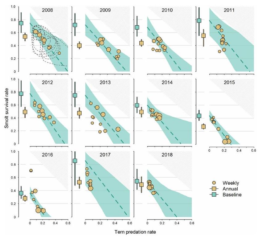
river (survival of smolts from Rock Island Dam [RIS] to BON), and SARs (survival from RIS to
adult returns at BON). They used the slope-based definition of additivity and compensation,
which allows them to estimate degrees of additivity and compensation, not just presence or
absence. Because of this, they can estimate the full range of possible relationships from over-
compensation to super-additivity. Overall, the data, the model structure, and its
implementation are well described, but the model is complicated, and it is difficult to assess all
the assumptions that may affect results.
Analysis of avian predation requires sufficient sample sizes to detect additivity or
compensation. Low returns are a problem with both studies, but it is especially acute in Payton
et al. (2020), especially later in the time series, because they analyze within-year patterns of
survival. Sample size is a major limitation for analysis of adult returns, which are very low
(including zero) in several years. This can lead to wide confidence intervals in results, but also
may lead to problems in interpretation of slopes in those years. The hierarchical model “shares”
data across years, which means years with higher returns could influence the slope estimates in
poor data years.
Payton et al. appears to show a consistent correlation between tern predation probability and
annual survival probability over the RIS-BON outmigration segment, perhaps because of
correlations induced by estimating both variables within the same multinomial model (Fig. 3).
For example, results from 2017 may be an artefact of the hierarchical structure imposed on the
a term so that a few years with a strong correlation “impose” it on the rest of the years (albeit
with a wider CI). The single high point in 2016 is also an outlier, and it would be worthwhile to
explore the reasons for that point. Figure 4 appears to show some relationship between tern
predation probability and SAR, although it is weaker than the relationship in the in-river
analysis. Some cohorts within a year are very flat (e.g., 2015) because virtually no adults
returned. Again, the hierarchical structure shares information across years, making it difficult to
evaluate individual year effects. The ISAB recommends that Payton et al. evaluate assumptions
and modeling of baseline survival.

 14

Figure 3. Weekly probability estimates of steelhead smolt survival and Caspian Tern predation
along with the estimated annual relationships between survival and predation during out-migra-
tion from Rock Island Dam to Bonneville Dam (Figure 3 in Payton et al. [2020]). The size of light
brown circles depicts relative numbers of steelhead smolts tagged and released each week at
Rock Island Dam. Approximate 95% credible regions are depicted for joint survival and predation
estimates in 2008 to demonstrate uncertainty, and error bars denote 95% CRI.

 15

Figure. 4. Estimated annual relationships between PIT-tagged steelhead smolt-to-adult survival
probabilities and Caspian Tern predation probabilities during smolt out-migration from Rock Is-
land Dam to the Pacific Ocean (Figure 4 in Payton et al. [2020]). The size of the light brown cir-
cles depicts the relative numbers of steelhead smolts tagged and released each week at Rock Is-
land Dam. Dashed lines represent the estimate of the best linear fit to the data and shading de-
notes 95% credible intervals (CRI) around the best fit. Annual estimates of survival with Tern pre-
dation (light brown box) and baseline survival in the absence of Tern predation (dark blue box)
are also provided (error bars denote 95% CRI).

Payton et al. found stronger evidence of additive mortality during in-river smolt migration than
either they or Haeseker et al. found for SAR. This may be due in part to the much larger
contrast in tern predation and in-river survival seen across cohorts in some years (Figure 3).
An additional issue arose late in the review process regarding potential biases in the tagging
groups used by Payton et al. (2020). This involved potential survival biases in steelhead tagged
at Rock Island Dam vs those tagged above Rocky Reach Dam. We examined the evidence
regarding the issue (Appendix B) and concluded that that there does not appear to be strong
evidence that tagging location bias affected estimation of the additivity coefficient or other
parameters in Payton et al. (2020) in a way that would invalidate conclusions and
interpretation, especially at the smolt to adult return (SAR) life stage. Nonetheless, the ISAB
recommends that possibilities for survival bias associated with tagging and release localities,
especially across cohorts within year be thoroughly evaluated.

 16

In summary, while both studies have potential issues in modeling and treatment of data (e.g.,
untested assumptions), both are scientifically sound analyses that use reasonable treatment,
processing, and modeling of their respective datasets.

2. Were the conclusions drawn by Haeseker et al. 2020 and Payton et al. 2020 analyses
 supported by their results?
Payton et al. (2020) estimated the parameter a, which measures the degree of additivity of
mortality due to avian predation for cohort and averaged across cohorts each year. Values of a
 0 were interpreted as over- and fully compensatory response of steelhead survival to avian
predation. Positive values of a were interpreted as partial additivity (0 < a < 1) and super
additivity (a > 1). They also estimated mortality from avian predation in excess of baseline
mortality. They concluded that avian predation was super-additive in-river (smolts RIS to BON),
and partially additive for SARs (smolts at RIS to adults at BON). Both conclusions are well
supported by their results.
Haeseker et al. (2020) conclude that predation in the estuary is consistent with full
compensation when considered at the SAR (BON smolts to BON adults) scale. This conclusion,
as stated, is supported by their analysis. However, in their discussion they assume that their
results, being consistent with full compensation, implies that they are inconsistent with
additivity. In this, they fall into the common statistical fallacy that failure to reject the null
hypothesis (that correlations are zero) implies that all alternative hypotheses are false. They
clearly state this fallacy in their methods: "We interpreted estimates of ρc near zero with
credible intervals that overlapped zero as indicating compensatory mortality, and we
interpreted negative estimates of ρc with credible intervals that did not overlap zero as
indicating additive mortality." This means that they depended on finding a significantly negative
correlation of adult survival and avian predation to infer additivity. In other words, they require
stronger evidence to accept additivity than to accept compensation. Under this standard, any
data set for which there are sufficiently wide error intervals would lead inevitably to a
conclusion of compensation whereas the reason would be variability in the data. Examination
of the credible intervals for their correlation estimates (their Tables 2 and 3) for their best
model include zero (thus being consistent with full compensation), but also include a range of
negative values (thus being consistent with some degree of additivity). In fact, for terns, their
mean estimate is slightly negative, providing more evidence for some degree of additivity than
for full compensation. For the above reasons, the ISAB finds that results and conclusions of
Haeseker et al. are consistent with full compensation but are not inconsistent with partial
additivity. Given these alternative interpretations, we suggest that conclusions be used
cautiously. A practical question is whether there is a material difference in outcomes that
depend on a finding of full compensation versus partial additivity in terms of expected effects

 17

of avian predator management on adult returns. Resolving this question requires further
analysis described in our response to Question 5.

3. How do the modeling approaches of Haeseker et al. 2020 and Payton et al. 2020 differ, and
 do these analytical differences or other reasons account for the contrasts in their
 conclusions?
The major differences in approach were discussed above. To summarize, the approaches
differed in:

 • Definitions of additivity and compensation: Haeseker et al. used a definition based on
 the simple correlation between predation and survival, while Payton et al. used a
 definition based on the initial slope of a piecewise relationship between predation and
 survival.

 • Populations considered: Haeseker et al. analyzed Snake River steelhead, while Payton
 et al. analyzed Upper Columbia River steelhead. There may be different rates of
 predation between these two drainages, but Payton et al. (2021) reported similar values
 for steelhead survival and tern predation in both basins.

 • Time period of observations: The time series only partially overlap – Haeseker et al.
 examined SAR for smolts from 2000 to 2015, Payton et al. examined in-river survival for
 smolts from 2008 to 2018, and SAR from 2008 to 2016. Population and predation levels
 vary from year to year, and this may affect estimates of correlations or regression
 slopes.

 • Life-cycle domain: Payton et al. evaluated avian predation relative to both in-river smolt
 survival (RIS to BON) and SAR (RIS smolts to BON adult returns), whereas Haeseker et al.
 only evaluated predation effects on SAR (BON smolts to BON adults).

 • Details of the models: The models differed in some details, notably pooling of estimates
 (Haeseker et al. estimated correlation across all years combined, Payton et al. estimated
 the additivity parameter (a) for each year), and inclusion of environmental covariates
 (Haeseker et al. included them; Payton et al. did not).
Any of these differences could lead to differences in conclusions, and it is not possible to
evaluate which are most important without side-by-side comparison of the models for the
same data sets, ideally including sensitivity analyses for main assumptions of each model. The
fundamental definitions used may lead to different biases and thus different conclusions. The
correlation-based definition used by Haeseker et al. may be problematic in ignoring the
constraints on additivity of predation that are accounted for in the piecewise regression

 18

definition of Payton et al. (see Appendix A for details). Use of correlation also can confuse the
issues of mean effect and variability about that mean because a low correlation cannot
distinguish between a lack of an effect or high variability (either process variation or sampling
error).
Different populations may have different inherent ecology surrounding predation, or there may
simply be different levels of predation and survival and variability in the two that affects data
contrasts and thus the ability (statistical power) to detect effects. The same problems could
arise from differences in the time periods examined in the two studies.
Differences in life-cycle stages analyzed by the two studies can also explain the different
conclusions. Haeseker et al. looked only at marine survival from BON smolts to BON adults,
while Payton et al. looked at two overlapping life stages: first, in-river migration from RIS smolts
to BON smolts, then total survival (SAR) from RIS smolts to BON adults. Haeseker et al. conclude
that predation effects on marine survival are consistent with their compensation hypothesis but
fail to note that they are also consistent with partial additivity (see discussion under Question
2) for this life stage. Payton et al. conclude that there is super-additivity in the effect of
upstream predation on in-river survival and partial additivity for the effect when in-river and
marine survival are combined. In fact, Payton et al. state that "[o]ver a scale as large as SARs,
representing the vast majority of an anadromous salmonid’s potential lifespan, any source of
mortality encountered early on will be mostly compensatory."
It is noteworthy that their conclusions are not inconsistent because of the differences in life-
cycle domains of the two studies. Haeseker et al. did not look at in-river survival, and therefore
did not produce results related to the conclusion of super-additivity during that life stage in
Payton et al. Similarly, Payton et al. looked at SARs from RIS to BON, which includes in-river
survival, and therefore did not produce results for the same spatial extent of the for BON-BON
SARs in Haeseker et al. For BON-BON SARs, where they do overlap, both studies are consistent
with either full compensation or a low degree of partial additivity in the marine environment.
Moreover, the Payton et al. result of partial additivity for in-river + marine survival could result
from super-additivity in the in-river stage being partially offset by full compensation or a low
degree of partial additivity in the marine stage.
Details of the models and their implementation also raise a number of possible reasons for
different results. However, the analyses were done separately and thus it is difficult to separate
data differences from statistical method differences. Somewhere in the mix of data and
methods, one can pinpoint WHY differences arose. This has not been done to date. Such inter-
analysis comparisons were started to be investigated in the Chapter 8 of the Avian Predation
Synthesis Report (Payton et al. 2021). However, this was mostly a verbal argument as to why
there are differences in the results of the two analyses and was from one set of authors. What

 19

is needed is a more rigorous comparison where the two methods are applied to the same data,
and each method is applied to the other study’s dataset. One can then begin to disentangle
how data and method differences contribute to the differences in results. These known
differences can then be transparently judged, and the results used to inform better
management actions.
Some major issues to investigate would be to compare how both analyses estimated the
predation effect from bird data, the temporal and spatial scaling of matching the bird pressure
with the steelhead survival, and use of covariates. Part of this is to compare the responses and
explanatory variables and their interpretation.
One conclusion that is clear (and likely obvious) is that bird predation is a major factor for some
years and for some stocks (see chapters for other stocks than steelhead in the Avian Predation
Synthesis Report [Roby et al. 2021]). The next level of interpretation (compensatory, additive)
depends on the shape of the relationship and is much less certain. This is expected because the
analysis to determine the amount of predation relies on the general magnitude while analysis
of the shape of the survival relationship requires additional confidence on how estimates of
survival vary across a range of bird predation rate.

4. Does the ISAB have recommendations to improve the analysis?
The ISAB recommends that both approaches be employed in side-by-side analysis of the same
datasets (possibly including simulated datasets where the “true” answer is known) to
simultaneously evaluate robustness to assumptions, statistical power, interpretations of each
modeling framework. Side-by-side analysis could discern whether differences in model design
and analytical power, or differences in location and population studied are most important in
explaining alternative interpretations and conclusions of these studies. This is the best way to
resolve issues of definitions, methodology, and data differences that limit comparison of the
results and conclusions of these two studies.
The ISAB recommends that future studies have better focus on management-related results
rather than on estimating degrees of additivity and compensation. While theoretically
important, the shape of the survival predation relationship is less important for management
than estimates of the actual effect of in-river predation on adult returns. Payton et al. (2020)
address the actual effect in their estimate of average annual SAR with or without predation
(their Δ ), but this could be improved for example by incorporating “adult equivalents” to put
super-additive mortality above BON into context with survival over entire life cycle, and by
providing independent estimates of baseline survival. As part of this recommendation, we
reiterate the recommendation from the ISAB Predation Metrics Report (ISAB 2016) to
encourage the use of comparable metrics with clear management implications as analysis

 20

endpoints, including equivalence-factor metrics (for example, adult equivalents) and a change
in population growth rate metric (aka delta-lambda, Δλ). Integration of avian predation findings
with life cycle modeling efforts to understand how other environmental correlates potentially
interact with susceptibility to avian predation could provide an important management tool
Both analyses also could be improved by examining several aspects of model formulation and
implementation. First is the question of bias in the analyses. Haeseker et al. rely on an earlier
study (Otis and White 2004) to indicate that their approach would have low bias, but Otis and
White specifically excluded consideration of the logit-transform that Haeseker et al. used in
their analysis. This transformation results in some degree of bias in parameter estimates or
their credible intervals, but it is not known how large bias could be. Payton et al. did a
simulation study of their model and found some degree of bias, but do not discuss any bias
corrections in their results. Additional studies of bias and methods of correcting for it would
enhance the reliability of both studies.
Although both studies model the effects of multiple predators in the same location and life-
stage, their models do not include possible effects of ecological interactions among the
predators. Competition, interference, or synergisms among predators could play a role in
determining total mortality and might modify the conclusions regarding additivity or
compensation on local scales. Including such interactions in future models might be useful.
Neither model takes harvest of steelhead into account in their estimates of SAR. This may not
be a substantial source of mortality for these steelhead populations as compared to higher
rates of commercial harvest for other species. Harvest possibly could be as important as avian
predation on an adult-equivalent basis and may also be an additional source of year-to-year
variation in SAR. Estimates of non-treaty harvest impacts for winter steelhead range between
0.2% and 9.4% since 2000, while estimates for summer A-run steelhead range from 1.5% to
8.6% for hatchery-origin fish and from 0.4% to 1.7% for natural-origin fish (Joint Columbia River
Management Staff 2021, Tables 9 and 11a). Adjusting mortality estimates for losses to harvest
of adults could be useful, perhaps included as another category of predator. However, the lack
of PIT tag detections in the harvest could make this difficult.
Several further analyses should be conducted to help understand differences and similarities of
those approaches. A comparison of the assumptions in a table format would help highlight
similarities and differences between the two analyses. Our Table 1 above is a start; more details
would further enable identification of similarities and differences and inform a comparative
analysis of the two methods and datasets. Similarly, exchanging datasets and methods, as well
as applying both methods to the same dataset, would begin to separate the issues that
confound comparisons across results generated to date (independently) by the two analyses.

 21