Counterfactual Generation and Fairness Evaluation Using Adversarially Learned Inference
←
→
Page content transcription
If your browser does not render page correctly, please read the page content below
Counterfactual Generation and Fairness Evaluation
                                                   Using Adversarially Learned Inference
                                                                             Saloni Dash, Amit Sharma
arXiv:2009.08270v2 [cs.CV] 18 Dec 2020

                                                                                 Microsoft Research
                                                                                  Bangalore, India
                                                                t-sadash@microsoft.com, amshar@microsoft.com

                                                                                            Abstract
                                                   Recent studies have reported biases in machine learning image classifiers, especially against
                                               particular demographic groups. Counterfactual examples for an input—perturbations that change
                                               specific features but not others—have been shown to be useful for evaluating explainability and
                                               fairness of machine learning models. However, generating counterfactual examples for images is
                                               non-trivial due to the underlying causal structure governing the various features of an image. To be
                                               meaningful, generated perturbations need to satisfy constraints implied by the causal model. We
                                               present a method for generating counterfactuals by incorporating a known causal graph structure
                                               in a conditional variant of Adversarially Learned Inference (ALI). The proposed approach learns
                                               causal relationships between the specified attributes of an image and generates counterfactuals
                                               in accordance with these relationships. On Morpho-MNIST and CelebA datasets, the method
                                               generates counterfactuals that can change specified attributes and their causal descendants while
                                               keeping other attributes constant. As an application, we apply the generated counterfactuals from
                                               CelebA images to evaluate fairness biases in a classifier that predicts attractiveness of a face.

                                         1    Introduction
                                         A growing number of studies have uncovered systemic biases in machine learning image classifiers,
                                         particularly against marginalized demographic groups [Buolamwini and Gebru, 2018, Hendricks
                                         et al., 2018, Zhao et al., 2017, Bolukbasi et al., 2016]. To avoid such biases, it is important to
                                         explain a classifier’s predictions and evaluate its fairness.
                                              Given any pre-trained machine learning (ML) classifier, counterfactual reasoning is an impor-
                                         tant way to explain the classifier’s decisions and to evaluate its fairness. Counterfactual reasoning
                                         involves simulating an alternative input with some specific changes compared to the original input.
                                         For example, to evaluate fairness of a classifier with respect to a sensitive attribute like skin color,
                                         we can ask how the classifier’s output will change if a face that was originally dark skinned is made
                                         light skinned while keeping everything else constant. Since the only change to the input is the sen-
                                         sitive attribute, counterfactual reasoning is considered more robust than comparing available faces
                                         with different skin colors in the dataset (association) or comparing simulated inputs with light skin
                                         or dark skin (intervention) since these comparisons may include other changes in addition to skin
                                         color. For tabular data, generating such counterfactual examples translates to simply changing a spe-
                                         cific feature (and other features caused by it [Mahajan et al., 2019]). As a result, the technique has
                                         found wide use in explaining ML classifiers [Kommiya Mothilal et al., 2019] and evaluating their
                                         fairness [Kusner et al., 2017].

                                         Explainable Agency in Artificial Intelligence Workshop, AAAI 2021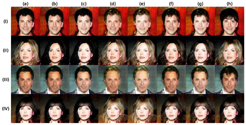
However, generating counterfactual examples for images is non-trivial. As a simple example,
consider the task of changing a person’s hair color in an image of their face. While Generative
Adversarial Networks (GANs) can generate new realistic faces with any hair color [Kocaoglu et al.,
2018], they are unable to generate the precise change needed for a counterfactual; change in hair
color without changing the hair style or other parts of the face. Other explanation techniques based
on perturbations such as occluding a grid of pixels [Zeiler and Fergus, 2014] are also insufficient for
counterfactual reasoning on high-level concepts.
     Formally, a counterfactual (CF) example for an image is defined with respect to a structural
causal model (SCM) over its attributes. Generating a counterfactual, therefore, requires modeling
both the underlying SCM for the attributes as well as the generative process that uses the attributes
to model the resulting image. In this paper we present ImageCFGen, a method that combines the
knowledge from a causal graph and uses an inference mechanism in a GAN-like framework to
generate the counterfactual images. Using these images, we show how to estimate the counterfactual
effect of each attribute on the target ML classifier’s output, and thereby evaluate fairness of the
classifier.
     To evaluate a given image classifier, the proposed method has two phases. In the first phase, we
train a generative model using Adversarially Learned Inference [Dumoulin et al., 2016] based on
observed attributes in the data. We assume a known SCM structure over attributes and its parameters
are learned from observed data or inferred based on domain knowledge. In the second phase, given
an image and the desired change, we modify its attributes based on the SCM and use them to generate
counterfactual images. To evaluate the image classifier’s properties, each counterfactual image is
input to the classifier and the associated output is compared to its output on the original image. We
show formally that our procedure satisfies the definition of a counterfactual as in [Pearl, 2009].
     The success of our method in evaluating image classifiers depends on the extent to which the
generated images correspond to the ideal counterfactual under the true SCM. We first evaluate Im-
ageCFGen on the Morpho-MNIST dataset to show that it generates counterfactual images com-
parable in quality to a prior CF generation method based on conditonal variational autoencoders
[Pawlowski et al., 2020]. Since ImageCFGen is GAN-based, our method has the advantage that
it is capable of generating high quality, realistic counterfactuals for complex datasets like CelebA
as compared to using VAEs which can produce blurry images due to conditional independence as-
sumptions [Goodfellow et al., 2014, Maaløe et al., 2016]. On CelebA, we demonstrate generating
CFs for facial attributes like Black Hair, Pale etc. Based on the counterfactual images, we find that
a standard image classifier for predicting attractiveness on the CelebA dataset exhibits bias w.r.t. to
Pale, but not w.r.t. other attributes like Narrow Eyes.
     To summarize, we make the following contributions:
    • ImageCFGen, a novel method that uses inference in a GAN-like framework to generate coun-
      terfactuals based on attributes learned from a known causal graph.
    • Evaluating fairness and explaining image classifiers using counterfactual reasoning.

2    Related Work
Our work bridges the gap between generating counterfactuals and evaluating fairness of image clas-
sifiers.

                                                  2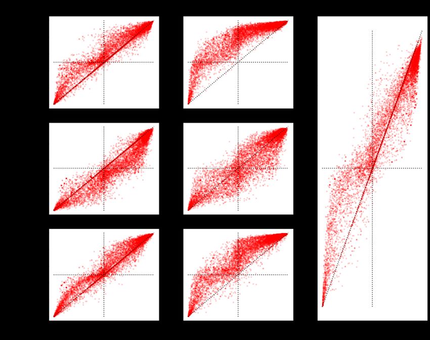
Generating Counterfactuals.
Suppose we want to generate a data point X (e.g., an image) based on a set of attributes A. Pearl’s
ladder of causation [Pearl, 2019] describes the three types of distributions that can be used: associ-
ation P (X|A = a), intervention P (X| do(A = a)) and counterfactual P (XA=a |A = a0 , X = x0 ).
The associational P (X|A = a) denotes the distribution of X when conditioned on a specific at-
tribute value a in the observed data. Conditional GAN based methods [Mirza and Osindero, 2014]
implement association between attributes and the image. The interventional P (X| do(A = a) de-
notes the distribution of X when A is changed to the value a irrespective of its observed associations
with other attributes. Methods like CausalGAN [Kocaoglu et al., 2018] learn an interventional distri-
bution of images after changing specific attributes and can generate new images that are outside the
observed distribution (e.g., women with moustaches on the CelebA faces dataset [Kocaoglu et al.,
2018]).
     The counterfactual P (XA=a |X = x0 , A = a0 ) denotes the distribution of images related to a
specific image x0 and attribute a0 , had the attribute of the same image been changed to a different
value a. In general, generating counterfactuals is a harder problem than generating interventional
data since we need to ensure that everything except the changed attribute remains the same between
an original image and its counterfactual. Pawlowski et al. [2020] proposed a method for generat-
ing image counterfactuals using a conditional VAE architecture. Since GANs have been used for
producing high quality images, we believe that a GAN based method will be optimal for modeling
complex image datasets, especially when the generated images need to be realistic to be used for
downstream applications such as fairness evaluation.
     Independent of our goal, there is a second interpretation of a “counterfactual” example w.r.t. a
ML classifier [Wachter et al., 2017], referring to the smallest change in an input that changes the
prediction of the ML classifier. Liu et al. [2019] use a standard GAN with a distance based loss to
generate CF images close to the original image. However, the generated CFs are not interpretable
and specific in their changes, and they do not consider the underlying causal structure. Ideally, a
counterfactual image should be able to change only the desired attribute while keeping the other
attributes constant.

Fairness of Image Classifiers.
There is a growing concern about biases against specific demographic populations in image classi-
fiers [Buolamwini and Gebru, 2018]. Methods have been proposed to inspect what features are con-
sidered important by a classifier [Sundararajan et al., 2017], constrain classifiers to give importance
to the correct or unbiased features [Ross et al., 2017], or enhance fairness by generating realistic
images from under-represented groups [McDuff et al., 2019]. Explanations can also be constructed
by perturbing certain parts of an image and checking whether the classifier changes its prediction,
e.g., by occluding an image region [Zeiler and Fergus, 2014] or by changing the smallest parts of an
image that change the classifier’s output [Fong and Vedaldi, 2017, Luss et al., 2019]. These pertur-
bations, however, do not capture high-level concepts of an image but rather change individual pixels
independently (or as a contiguous block of “super-pixels”).
     Perhaps closest to our work are two papers that use adversarially-trained generative models to
generate counterfactuals for a given image. Denton et al. [2019] change attributes for a given image
by linear interpolations of latent variables using a standard progressive GAN [Karras et al., 2018],
and [Joo and Kärkkäinen, 2020] use a Fader network architecture [Lample et al., 2017] to change
attributes. However, these works ignore the causal structure associated with attributes of an image. In
analyzing bias against an attribute, it is important to model the downstream changes due to changing
that attribute [Kusner et al., 2017]. For instance, for a chest MRI classifier, age of a person may affect

                                                    3
the relative size of their organs [Pawlowski et al., 2020]; it will not be realistic to analyze the effect
of age on the classifier’s prediction without learning the causal relationship from age to organ size.
Therefore, in this work we present a different architecture that can model the causal relationships
between attributes and provides valid counterfactuals w.r.t. an assumed structural causal model. In
addition, our method can generate counterfactuals for both sensitive and non-sensitive attributes and
thus be used for explaining a classifier, unlike the method in [Joo and Kärkkäinen, 2020].
3 Method
We now formulate the problem of counterfactual generation for images and describe how ImageCF-
Gen can generate counterfactuals and be used to evaluate fairness as well as explain a classifier.
Let X = x denote the image we want to generate the counterfactual for and let A = a = {ai }ni=1
be its corresponding attributes. Each ai can be a binary variable (∈ {0, 1}) or a continuous variable
(∈ R). A continuous attribute is scaled so that it lies in the range of [0, 1].
To generate a counterfactual for an image (x, a), the proposed method ImageCFGen has three
steps. The Encoder E infers the latent space distribution z from x and a. The Attribute SCM learns
the Structural Causal Model for the attributes a, intervenes on the desired subset of attributes, and
outputs ac according the learned SCM. (refer to Attribute SCM for more details). The Generator
G learns to map (z, a) back to x. The architecture for generating CFs is shown in Figure 1. For
our experiments, we use Adversarially Learned Inference [Dumoulin et al., 2016] to train the En-
coder and Generator. However, ImageCFGen can be extended to any Encoder-Decoder(Generator)
mechanism.
Figure 1: Counterfactual Generation using ImageCFGen. The top half of the figure shows the CF
generation procedure, where the Attribute SCM outputs ac after intervening on a subset of the at-
tributes a. The Generator G then generates the CF image xc given the latent space distribution z
from Encoder E and ac from Attribute SCM. The bottom half of the figure shows the reconstruction
procedure, where the G directly takes z from the E and the attributes a to generate the reconstructed
image xr . Finally, xr and xc are used for a downstream task like fairness evaluation of a classifier.
43.1 Attribute SCM
We model the relationship between attributes a using the Attribute SCM that consists of a causal
graph structure and associated structural assignments. We assume that the causal graph for at-
tributes is known, but the structural assignments need to be estimated. For instance, assuming two
attributes (Young, Gray Hair) for an image x of a face, the true causal graph can be assumed to
be Young → Gray Hair → x. We separate out the graph into two parts: relationships amongst the
attributes (Ma ), and relationships from the attributes to the image (Mx ). The Attribute SCM learns
the structural assignments between attributes (in this case, Gray Hair = f (Young, ) where denotes
independent random noise). These equations for the attributes can be estimated using Normalizing
Flows [Rezende and Mohamed, 2015, Pawlowski et al., 2020] or Maximum Likelihood Estima-
tion in Bayesian Networks [Ding, 2010]. Modeling the second part of the graph (relationships from
attributes to an image) requires a generator architecture that we describe next.
3.2 Adversarially Learned Inference
Many studies have reported generating high quality, realistic images using GANs [Wang et al., 2018,
Karras et al., 2018, 2019]. However, GANs lack an inference mechanism where the input x can be
mapped to its latent space representation z. Adversarially Learned Inference [Dumoulin et al., 2016]
integrates the inference mechanism of variational methods like VAEs in a GAN-like framework,
thereby leveraging the generative capacity of GANs as well as providing an inference mechanism.
We generate the images using a conditional variant of ALI so that the model can be conditioned
on the attributes a. ALI uses an Encoder E and a Generator G in an adversarial framework, where
the Encoder learns to approximate the latent space distribution from the input x and attributes a, and
the Generator learns to generate realistic images from the latent space distribution and attributes a.
The Discriminator D is optimized to differentiate between pairs of the real image, the correspond-
ing approximated latent space variable and attributes, from joint samples of the generated image, the
input latent variable and attributes, while in conjunction the Encoder and Generator are optimized to
fool the discriminator. In ALI the attributes are embedded in G, E and D using an embedding net-
work. However, we directly pass the attributes to the Generator, Encoder and Discriminator because
we found that it helped in conditioning the model on the attributes better as compared to embedding
it. The conditional ALI optimizes, [Dumoulin et al., 2016]:
min max V (D, G, E) = Eq(x)p(x) [log(D(x, E(x, a), a))]
G,E D
(1)
+Ep(z)p(a) [log(1 − D(G(z, a), z, a))]
G is the Generator, E is the Encoder and D is the discriminator. q(x) is the distribution for the
images, p(z) ∼ N (0, 1) and p(a) is the distribution of the attributes.
Image reconstructions are defined as,
xr = G(E(x, a), a), (2)
3.3 Counterfactual Generation
Let x be an image for which we want to generate counterfactuals and let a be its corresponding
attributes. Generating a CF for (x, a) requires three steps [Pearl, 2009]:
• Abduction: Infer latent z given the input (x, a) using the Encoder.
5• Action: Let ak ⊆ a be the set of k attributes that one wants to intervene on. Set attribute
ai → a0i ∀ai ∈ ak , given a0k = {a0i }ki=1 .
• Prediction: Modify all the descendants of ak according to the SCM equations learned by
Attribute SCM. This outputs ac , the intervened attributes. Use z from the Encoder and ac
from the Attribute SCM and input it to the generator to obtain the counterfactual xc .
Mathematically, a counterfactual can be generated using:
xc = G(E(x, a), ac ), (3)
where ac is computed using Attribute SCM, from a0k ; the set of all values that you want to change
the attributes in ak to.
The detailed steps are shown in Algorithm 1. Below we prove that the counterfactual generation
mechanism corresponds to generating a valid counterfactual.
Proposition 1. Assume that the true SCM M belongs to a class of SCMs where the structural
equations can be identified uniquely given the causal graph. Further, assume that the Encoder E,
Generator G and Attribute SCM are optimal and thus correspond to the true structural equations
of the SCM M. Then Equation 3 generates a valid counterfactual image for any given input (x, a)
and the requested modified attributes a0k .
Proof. Let M = {Mx , Ma } be the true SCM that generates the data (x, a). Let ak ⊂ a be the
attributes you want to intervene on. Let a−k = a\ak be the remaining attributes. The corresponding
equations for M are:
ai := gi (pai , i ), ∀i = 1..n
(4)
x := g(ak , a−k , )
where and i refer to independent noise, g and gi refer to structural assignments of the SCMs Mx
and Ma respectively while pai refers to parent attributes of ai . Given an input (x, ak , a−k ), we
generate a counterfactual using M and show that it is equivalent to Equation 3.
Abduction Infer for x and i for all ai from Equation 4 using the following equations:
ˆi := gi−1 (ai , pai ), ∀i = 1..n
−1
(5)
ˆ := g (x, ak , a−k )
Action Intervene on all attributes ak by setting them to the requested modified attributes a0k .
ai → a0i ∀ai ∈ ak and ∀a0i ∈ a0k (6)
Prediction The following equation then changes the values of all descendants of ak .
desc(ai ) → gi (pdesc(ai ) , ˆi ) ∀ai ∈ ak (7)
where desc(ai ) are descendants of ai and pdesc(ai ) are parents of the descendants of ai , ∀ai ∈ ak .
Let ac = a0k ∪ a0−k where a0−k are (possibly) modified values of the other attributes according to
Equation 7. Therefore, the counterfactual of x, xc can be generated as,
xc := g(ac , ˆ) (8)
We now show that Equation 3 produces the same xc . By the assumption in the theorem statement,
the Attribute SCM corresponds to the structural assignments {gi , gi−1 }, ∀i = 1..n of SCM Ma while
6the Generator G learns the structural assignment g and the Encoder E learns g −1 of the SCM Mx .
Hence, the Attribute SCM, Generator and Encoder learn the combined SCM M.
When the SCM assignments learned by the Attribute SCM are optimal, i.e. Attribute SCM =
Ma then:
âc = ac
Similarly, under optimal Generator, G = g and E = g −1 :
xc = g(ac , g −1 (x, ak , a−k ))
(9)
= G(ac , E(x, a)) (as a = ak ∪ a−k )
which is the same as Equation 3.
Algorithm 1: ImageCFGen
Input: (x, a), Attributes to Modify ak , Modified Attribute Values a0k , Attribute SCM Ma ,
Encoder E, Generator G
Output: xc
1 Abduction: z = E(x, a)
0 0 0
2 Action: ai → ai ∀ai ∈ ak
3 Prediction:
4 foreach ai ∈ ak do
5 foreach descendant of ai desc(ai ) do
6 desc(ai ) → gi (pdesc(ai ) , ˆi ) ∀ai ∈ ak
7 end
8 end
0 0
9 ac = ak ∪ a−k
10 xc = G(z, ac )
3.4 Fairness Analysis
We can use the generated CFs to estimate biases in a given classifier that predicts whether a face
is attractive or not. We compare classification labels for reconstructed images ( xr from 2) and
counterfactual images (xc from 3), since the reconstructed images share the exact same latent z as
the counterfactual image (which the original image may not share, since model reconstructions are
not perfect). Since the CFs are with respect to the reconstructed images we refer to the reconstructed
images as original images throughout the paper. We characterize the classifier as biased if (a) it
changes it’s classification label for the counterfactual image and b) if it changes the label to one
class from another class more often than vice-versa. We summarise these intuitions as a formula for
the degree of bias in a binary classifier,
bias = p(yr 6= yc )(p(yr = 0, yc = 1|yr 6= yc )
(10)
−p(yr = 1, yc = 0|yr 6= yc )),
where yr is the classification label for the reconstructed image, yc is the classification label for the
counterfactual image. Using Bayes Theorem Equation 10 reduces to
bias = p(yr = 0, yc = 1) − p(yr = 1, yc = 0) (11)
7The bias defined above ranges from -1 to 1, where it is 0 in the ideal scenario when the probability
of CF label changing from 0 to 1 and vice-versa (changing from 1 to 0 ) is the same (=0.5). The bias
value is 1 in the extreme case when the CF label always changes to 1, suggesting that the classifier is
biased towards the counterfactual change. Similarly in the case that the CF label always changes to
0, the bias will have a value of -1, suggesting that the classifier is biased against the counterfactual
change.
We also show that a classifier with zero bias metric is fair w.r.t. to the formal definition of
counterfactual fairness.
Definition 1. Counterfactual Fairness from [Kusner et al., 2017]. Let A be the set of attributes,
comprising of sensitive attributes AS ⊆ A and other non-sensitive attributes AN . Classifier Ŷ is
counterfactually fair if under any context X = x and A = a, changing the value of the sensitive
features to AS ← a0s counterfactually does not change the classifier’s output distribution.
P (ŶAS ←as = y|X = x, AS = as , AN = aN )
(12)
= P (ŶAS ←a0s = y|X = x, AS = as , AN = aN )
for all y and for any value a0s attainable by AS .
Proposition 2. Under the assumptions of Proposition 1 for the Encoder E, Generator G, and At-
tribute SCM Ma ,, a classifier fˆ : X → Y that satisfies zero bias according to Equation 10 is
counterfactually fair with respect to M.
Refer to suppl. for the proof.
3.5 Explaining a Machine Learning Classifier
We can also use the counterfactuals to generate explanations for a classifier. For any input x, a local
counterfactual explanation states how the classifier’s prediction changes upon changing a specific
attribute. We write it as,
E[ŶA←a0 |(x, a)] − E[ŶA←a |(x, a)]
where, for a binary attribute, a0 = 1 and a = 0.
4 Evaluation
We describe our results on two datasets, Morpho-MNIST and CelebA. We use Morpho-MNIST to
evaluate the quality of generated counterfactuals in comparison to prior work [Pawlowski et al.,
2020], and CelebA to show how generated CFs can be used to evaluate fairness and explain the
decisions of a image classifier. We plan to make our code available on GitHub for reproducibility.
• Morpho-MNIST. Morpho-MNIST [Castro et al., 2019] is a publicly available dataset that
generates synthetic digits based on MNIST [LeCun et al., 1998] with interpretable attributes
like thickness, slant etc. Pawlowski et al. [2020] extend Morpho-MNIST by introducing mor-
phological transformations to generate a dataset with a known causal graph. The attributes
included in this variant of Morpho-MNIST are thickness and intensity, where thickness →
intensity. We append to this dataset by introducing an independent morphological attribute—
slant from the original Morpho-MNIST dataset and include digit label as an attribute as ell.
The causal graph for the dataset used is given in Figure 2.
8Figure 2: Causal graph for Morpho-MNIST. The attributes, thickness t, intensity i, slant s and label
l, cause the image x.
• CelebA. CelebA [Liu et al., 2015] is a dataset of around 200k celebrity images annotated with
40 attributes like Black Hair, Wearing Hat, Smiling etc. All attributes (excluding Attractive)
are used to train an image classifier that predicts the attribute Attractive. However, for fairness
evaluations we only generate CFs for the attributes Black Hair, Blond Hair, Brown Hair,
Pale and Bangs. While explaining the classifier’s decisions, we generate CFs for all attributes
excluding Male, Young and Blurry. Like Denton et al. [2019], we do not generate CFs for Male
because of inconsistent social perceptions surrounding gender, thereby making it difficult to
define a causal graph not influenced by biases. Therefore all the attributes we consider have a
clear causal structure (refer to suppl. for the causal graph).
Details of the implementation, architecture and training are provided in the suppl.
4.1 Counterfactual Evaluation with Morpho-MNIST
We train ImageCFGen on our causal version of Morpho-MNIST (as described above). Before gen-
erating CFs, we qualitatively evaluate the Encoder by sampling images along with their attributes
from the test set and passing them through the encoder to obtain their latent space representations.
These representations are passed to the generator which outputs reconstructions of the original im-
age. The reconstructions are showed in Figure 3. Overall, reconstructions for Morpho-MNIST are
faithful reproductions of the real images.
We then generate counterfactuals using the method described in the previous section. We inter-
vene on all four attributes - thickness, intensity, slant and label and observe how the image changes
with these attributes. Figure 4 demonstrates counterfactuals for a single image with label 0. Along
the first column vertically, the label is changed from 0 to {1, 4, 6, 9} while the thickness, intensity
and slant are kept constant. Then, as we proceed to the right in each row, the attributes of thickness,
intensity and slant are changed sequentially but the label is kept constant. Visually, the generated
counterfactuals change appropriately according to the intervened attributes.For instance, according
to the causal graph in Figure 2, changing the digit label should not change the digit thickness inten-
sity and slant. That is precisely what is observed in column (a) of Figure 4. Whereas, changing the
thickness should also change the intensity of the image which is observed in columns (c) and (d) of
Figure 4.
9Figure 3: Morpho-MNIST Reconstructions. Odd columns denote real images sampled from the test
set, and even columns denote reconstructions for those real images.
Figure 4: Morpho-MNIST Counterfactuals. (Ia) is a real image sampled from the test set. Rows
(II), (III), (IV) and (V) correspond to do(label = 1), do(label = 4), do(label = 6) and do(label = 9)
respectively. Columns (b), (c), (d) correspond to interventions on thickness: do(t = 1), do(t = 3) and
do(t = 5) respectively. Similarly, (e), (f) and (g) correspond to interventions on intensity: do(i = 68),
do(i = 120), do(i = 224) respectively. Finally, columns (h), (i) and (j) correspond to interventions on
slant: do(s = -0.7), do(s = 0) and do(s = 1).
To quantitatively evaluate the efficacy of the CFs, we randomly sample hundred values for thick-
ness, intensity and slant attributes and generate corresponding CFs for each test image. We plot the
target ground truth attribute vs the measured attribute in the CF image in Figure 5. All attributes
are on an average clustered along the reference line of y = x with some variability. We quantify
this variability in Table 1 using median absolute error, where we compare the CFs generated us-
ing ImageCFGen vs the CFs generated using DeepSCM method of Pawlowski et al. [2020]. We
choose Median Absolute Error to capture the overall behaviour of the CFs and not have outliers
skew the measurements. Overall ALI and DeepSCM are comparable on the attributes of thickness
and intensity. We could not compare slant since Pawlowski et al. [2020] do not use slant in their
experiments.
10Figure 5: Morpho-MNIST Empirical Analysis of CFs. The x axis is the target attibute while the y
axis is the measured attribute. In the ideal scenario, as shown with the real samples, the points should
lie along the y = x line. For the counterfactuals generated by ImageCFGen, the points roughly lie
along the diagonal.
do(thickness) do(intensity)
ImageCFGen 0.404 11.0
DeepSCM 0.258 12.4
Table 1: Median Abs. Error: ImageCFGen and DeepSCM.
4.2 Fairness Evaluation with CelebA
We apply our method of CF generation to the CelebA dataset and use the CFs to evaluate biases
in a classifier that predicts whether a face is attractive or not. Details of training the attractiveness
classifier are in the Suppl. Specifically, we intervene on the attributes of Black Hair, Blond Hair,
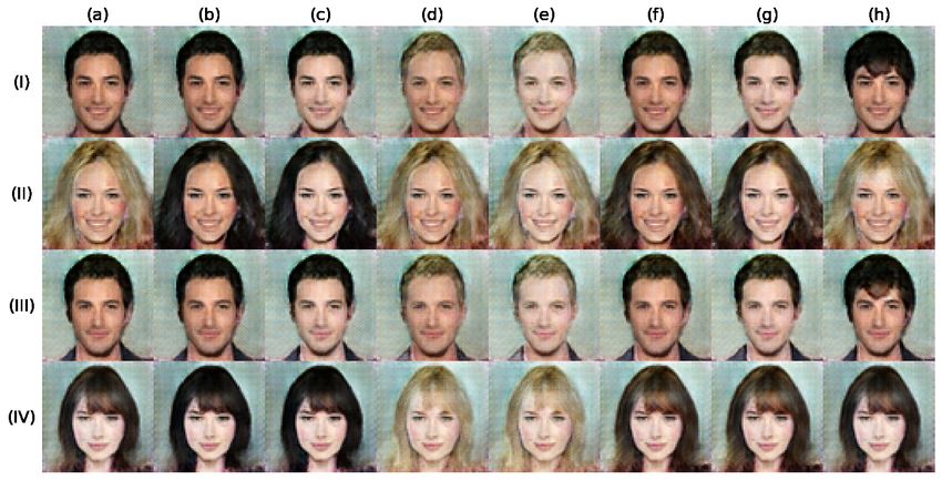
Brown Hair, Pale and Bangs to generate the CF images. The generated CFs are shown in Figure 6.
Note how the CF image is different with respect to the original image only in terms of the intervened
attribute. Consequently, if the attribute in the original image is already present, the CF image is
exactly the same as the original image. For instance, for (Ia) and (Ib) in Figure 6 are exactly the
same since the original image (Ia) already has black hair, hence intervening on black hair has no
effect on it. Similarly, in row IV, since the original image is already pale, intervening on pale in
columns (c), (e) and (g) has no effect. Additionally, since the original image already has bangs,
intervening on bangs in (h) has no effect.
We sample 10k points from the test set and generate seven CFs for each of them as shown in
Fig. 6. We only consider those images for which the corresponding attribute was absent in order
to avoid redundancies. For instance we filter out Ib from Figure 6 since black hair was already
present in the original image. We then provide the generated CFs along with the original image to
the attractive classifier and compare their labels. As a baseline comparison, we also pass images
with affine transformations like horizontal flip and increasing brightness to the classifier. We treat
the classifier’s outputs as the probability of being labelled as attractive. We plot these probabilities
for the original image, affine transformations, and the CFs. If the classifier is fair wrt these attributes,
11(a) Constant z
(b) Encoder z
Figure 6: CelebA Counterfactuals. Subfigure (a) reproduces conditional generation from [Dumoulin
et al., 2016] where attributes are varied for a constant z. Subfigure (b) demonstrates counterfactu-
als for reconstructed images, where the attributes are varied for the z taken from the Encoder (as
described in Method). For both the subfigures, (a) across all rows I, II, III, IV represent images
reconstructed from test samples. (b) denotes do(black hair = 1) and (c) denotes do(black hair = 1,
pale =1). Similarly (d) denotes do(blond hair = 1) and (e) denotes do(blond hair = 1, pale = 1) while
(f) denotes do(brown hair = 1) and (g) denotes do(brown hair = 1, pale = 1). Finally, (h) denotes
do(bangs = 1).
all points should be clustered along the y=x line.
For the CF plots, for do (black hair =1, pale = 1) and do (brown = 1, pale = 1) almost all points
are above the reference line, suggesting that the probability of being classified as attractive increases
after applying these interventions. Not only does the probability increase, for do (black hair = 1, pale
= 1), 18% of the CF labels are flipped from the original ones, and 99% of these labels are changed
from not attractive to attractive. In case of do(brown hair = 1, pale = 1), 17% of the CF labels are
flipped and 99% of the labels are flipped from not attractive to attractive. Interestingly, for the CF
do (blond hair = 1), the bias is in the opposite direction, where 89% of the labels are flipped from
attractive to not attractive. The affine transformations are unable to provide a clear picture of bias.
We quantify these observations according to Equation 10 in Table 2. The degree of bias for-
12(a) Affine transformations
(b) Counterfactuals
Figure 7: Fairness Analysis. Each point in a scatter plot is a pair of an original image and its cor-
responding CF image. Each scatter plot can be divided into four quadrants formed by the lines x =
0.5 and y = 0.5. Starting from the top left quadrant (x < 0.5, y > 0.5), any point lying in this region
signifies that the attractive label was changed from 0 to 1 for the corresponding CF. Similarly, the
CF label for points in the bottom right quadrant(x > 0.5 and y < 0.5) was changed from 1 to 0. For
the points lying in the top right and bottom left quadrants, the CF label stays the same.
mulation gives an overall estimation of the bias present in the classifier, and gives an interpretable
and uniform scale to compare biases amongst different classifiers. Overall in Table 2 the bias values
correspond to the intuitions developed from Figure 7. We observe that the CF of do (black hair =
1, pale = 1) has the highest positive bias amongst all the CFs and affine transformations while do
(blond hair = 1) has the highest negative bias amongst all the CFs. The significant biases we observe
are for the CFs of setting pale as true for hair colors brown and black, where the classifier is biased
towards labelling these CFs as more attractive in contrast to the original image, while for setting
the hair as blond, the classifier is more prone to changing the label from attractive to not attractive.
Moreover, for the baseline transformations the calculated biases are negligible.
We also use CFs to explain the classifier’s decisions for predicting attractive / not attractive.
13p(ar 6= ac ) p(0 → 1) bias
Horizontal Flip 0.071 0.496 0.000
Brightness 0.137 0.619 0.033
black h 0.067 0.838 0.045
black h, pale 0.177 0.996 0.175
blond h 0.090 0.115 - 0.069
blond h, pale 0.095 0.773 0.052
brown h 0.057 0.877 0.043
brown h, pale 0.165 0.999 0.165
bangs 0.084 0.845 0.058
Table 2: Bias Estimation. Bias values above a threshold of 5% are considered significant.
Figure 8 shows the top 5 positive and top 5 negative influences for classifying a face as attractive.
We can see that Pale is the top attribute that contributes to the classifier predicting a face as attrac-
tive, while Receding Hairline is the top attribute that contributes to the classifier prediction of not
attractive
Figure 8: Explaining a Classifier. Attribute ranking of top 5 positive and top 5 negative influential
attributes.
Additionally, our method can also be utilized in the setting where the attributes are connected
in a complex causal graph structure, unlike [Denton et al., 2019, Joo and Kärkkäinen, 2020]. We
conduct a similar fairness and explanation analysis for a Attractive classifier in the suppl., where
Young affects other visible attributes like Gray hair.
5 Conclusion
We propose a novel framework ImageCFGen that not only leverages the generative capacity of
GANs but also utilizes an underlying SCM for generating counterfactuals. We demonstrate how the
counterfactuals can be used to analyse fairness as well as explain an image classifier’s decisions.
6 Ethical Statement
This work focuses on the ethical issues of using a machine learning classifier on images, especially
on images related to people such as their faces. Techniques that aid researchers in interpreting an im-
14age classifier can be useful for detecting potential biases in the model. Accurate estimates of fairness
biases can also help in evaluating the utility of an image classifier in particularly sensitive settings
and minimize potential harm that could be caused if the model is deployed. With this motivation, we
propose a method for generating counterfactual images that change only certain attributes for each
image in the data. Such counterfactual images have been shown to be useful for identifying bias and
explaining which features are considered important for a model. By extending the CF generation to
images, we hope that our method can be useful in detecting biases in image classifiers.
However, we acknowledge that there are many challenges in generating meaningful and realistic
counterfactuals, and without proper consideration, our method can lead to incorrect conclusions and
potential harm. First, our method relies on knowledge of the true causal graph. In applications like
face classifiers, it can be very difficult to obtain a true causal graph. In addition, as Denton et al.
[2019] argue, generating counterfactual images for gender may be a misguided exercise since many
associations with facial features to gender are socially constructed, and thus may reinforce stereo-
types. Second, our method for generating an image based on the attributes relies on a statistical
model that can have have unknown failure modes. A potential harm is that the CF generation model
may make some approximations (or may have biases of its own) that render the counterfactual anal-
ysis invalid. This work should be considered as a prototype early work in generating counterfactuals
and is not suitable for deployment.
References
M. Abadi, P. Barham, J. Chen, Z. Chen, A. Davis, J. Dean, M. Devin, S. Ghemawat, G. Irving, M. Is-
ard, et al. Tensorflow: A system for large-scale machine learning. In 12th {USENIX} Symposium
on Operating Systems Design and Implementation ({OSDI} 16), pages 265–283, 2016.
T. Bolukbasi, K.-W. Chang, J. Y. Zou, V. Saligrama, and A. T. Kalai. Man is to computer programmer
as woman is to homemaker? debiasing word embeddings. In Advances in neural information
processing systems, pages 4349–4357, 2016.
J. Buolamwini and T. Gebru. Gender shades: Intersectional accuracy disparities in commercial
gender classification. In Conference on fairness, accountability and transparency, pages 77–91,
2018.
D. C. Castro, J. Tan, B. Kainz, E. Konukoglu, and B. Glocker. Morpho-mnist: Quantitative as-
sessment and diagnostics for representation learning. Journal of Machine Learning Research, 20
(178):1–29, 2019.
F. Chollet et al. Keras. https://keras.io, 2015.
E. Denton, B. Hutchinson, M. Mitchell, and T. Gebru. Detecting bias with generative counterfactual
face attribute augmentation. arXiv preprint arXiv:1906.06439, 2019.
J. Ding. Probabilistic inferences in bayesian networks. InA. Rebai (ed.), Bayesian Network, pages
39–53, 2010.
V. Dumoulin, I. Belghazi, B. Poole, O. Mastropietro, A. Lamb, M. Arjovsky, and A. Courville.
Adversarially learned inference. arXiv preprint arXiv:1606.00704, 2016.
R. C. Fong and A. Vedaldi. Interpretable explanations of black boxes by meaningful perturbation. In
Proceedings of the IEEE International Conference on Computer Vision, pages 3429–3437, 2017.
15I. Goodfellow, J. Pouget-Abadie, M. Mirza, B. Xu, D. Warde-Farley, S. Ozair, A. Courville, and
Y. Bengio. Generative adversarial nets. In Advances in neural information processing systems,
pages 2672–2680, 2014.
L. A. Hendricks, K. Burns, K. Saenko, T. Darrell, and A. Rohrbach. Women also snowboard:
Overcoming bias in captioning models. In European Conference on Computer Vision, pages
793–811. Springer, 2018.
J. Joo and K. Kärkkäinen. Gender slopes: Counterfactual fairness for computer vision models by
attribute manipulation. arXiv preprint arXiv:2005.10430, 2020.
T. Karras, T. Aila, S. Laine, and J. Lehtinen. Progressive growing of gans for improved quality,
stability, and variation. In International Conference on Learning Representations, 2018.
T. Karras, S. Laine, and T. Aila. A style-based generator architecture for generative adversarial
networks. In Proceedings of the IEEE conference on computer vision and pattern recognition,
pages 4401–4410, 2019.
D. P. Kingma and J. Ba. Adam: A method for stochastic optimization. arXiv preprint
arXiv:1412.6980, 2014.
M. Kocaoglu, C. Snyder, A. G. Dimakis, and S. Vishwanath. Causalgan: Learning causal implicit
generative models with adversarial training. In International Conference on Learning Represen-
tations, 2018.
R. Kommiya Mothilal, A. Sharma, and C. Tan. Explaining machine learning classifiers through
diverse counterfactual explanations. arXiv, pages arXiv–1905, 2019.
M. J. Kusner, J. Loftus, C. Russell, and R. Silva. Counterfactual fairness. In Advances in neural
information processing systems, pages 4066–4076, 2017.
G. Lample, N. Zeghidour, N. Usunier, A. Bordes, L. Denoyer, and M. Ranzato. Fader networks:
Manipulating images by sliding attributes. In Advances in neural information processing systems,
pages 5967–5976, 2017.
Y. LeCun, L. Bottou, Y. Bengio, and P. Haffner. Gradient-based learning applied to document recog-
nition. Proceedings of the IEEE, 86(11):2278–2324, 1998.
S. Liu, B. Kailkhura, D. Loveland, and Y. Han. Generative counterfactual introspection for ex-
plainable deep learning. In 2019 IEEE Global Conference on Signal and Information Processing
(GlobalSIP), pages 1–5. IEEE, 2019.
Z. Liu, P. Luo, X. Wang, and X. Tang. Deep learning face attributes in the wild. In Proceedings of
International Conference on Computer Vision (ICCV), December 2015.
R. Luss, P.-Y. Chen, A. Dhurandhar, P. Sattigeri, Y. Zhang, K. Shanmugam, and C.-C. Tu. Generating
contrastive explanations with monotonic attribute functions. arXiv preprint arXiv:1905.12698,
2019.
L. Maaløe, C. K. Sønderby, S. K. Sønderby, and O. Winther. Auxiliary deep generative models.
In Proceedings of the 33rd International Conference on International Conference on Machine
Learning-Volume 48, pages 1445–1454, 2016.
16D. Mahajan, C. Tan, and A. Sharma. Preserving causal constraints in counterfactual explanations
for machine learning classifiers, 2019.
D. McDuff, S. Ma, Y. Song, and A. Kapoor. Characterizing bias in classifiers using generative
models. In Advances in Neural Information Processing Systems, pages 5403–5414, 2019.
M. Mirza and S. Osindero. Conditional generative adversarial nets. arxiv 2014. arXiv preprint
arXiv:1411.1784, 2014.
N. Pawlowski, D. C. Castro, and B. Glocker. Deep structural causal models for tractable counter-
factual inference. arXiv preprint arXiv:2006.06485, 2020.
J. Pearl. Causality. Cambridge university press, 2009.
J. Pearl. Bayesian networks. 2011.
J. Pearl. The seven tools of causal inference, with reflections on machine learning. Communications
of the ACM, 62(3):54–60, 2019.
D. J. Rezende and S. Mohamed. Variational inference with normalizing flows. In Proceedings of
the 32nd International Conference on International Conference on Machine Learning-Volume 37,
pages 1530–1538, 2015.
A. S. Ross, M. C. Hughes, and F. Doshi-Velez. Right for the right reasons: training differentiable
models by constraining their explanations. In Proceedings of the 26th International Joint Confer-
ence on Artificial Intelligence, pages 2662–2670, 2017.
M. Sundararajan, A. Taly, and Q. Yan. Axiomatic attribution for deep networks. In Proceedings of
the 34th International Conference on Machine Learning-Volume 70, pages 3319–3328, 2017.
S. Wachter, B. Mittelstadt, and C. Russell. Counterfactual explanations without opening the black
box: Automated decisions and the gdpr. Harv. JL & Tech., 31:841, 2017.
T.-C. Wang, M.-Y. Liu, J.-Y. Zhu, A. Tao, J. Kautz, and B. Catanzaro. High-resolution image syn-
thesis and semantic manipulation with conditional gans. In Proceedings of the IEEE conference
on computer vision and pattern recognition, pages 8798–8807, 2018.
M. D. Zeiler and R. Fergus. Visualizing and understanding convolutional networks. In European
conference on computer vision, pages 818–833. Springer, 2014.
J. Zhao, T. Wang, M. Yatskar, V. Ordonez, and K.-W. Chang. Men also like shopping: Reducing
gender bias amplification using corpus-level constraints. In Proceedings of the 2017 Conference
on Empirical Methods in Natural Language Processing, pages 2979–2989, 2017.
177 Counterfactual Fairness Proof
Definition 1. Counterfactual Fairness from [Kusner et al., 2017]. Let A be the set of attributes,
comprising of sensitive attributes AS ⊆ A and other non-sensitive attributes AN . Classifier Ŷ is
counterfactually fair if under any context X = x and A = a, changing the value of the sensitive
features to AS ← a0s counterfactually does not change the classifier’s output distribution.
P (ŶAS ←as = y|X = x, AS = as , AN = aN )
(12)
= P (ŶAS ←a0s = y|X = x, AS = as , AN = aN )
for all y and for any value a0s attainable by AS .
Proposition 2. Under the assumptions of Proposition 1 for the Encoder E, Generator G, and At-
tribute SCM Ma ,, a classifier fˆ : X → Y that satisfies zero bias according to Equation 10 is
counterfactually fair with respect to M.
Proof. To evaluate fairness, we need to reason about the output Y = y of the classifier fˆ. Therefore,
we add a functional equation to the SCM M from Equation 4.
ai := gi (pai , i ), ∀i = 1..n
x := g(ak , a−k , ) (13)
y ← fˆ(x)
where and i are independent errors as defined in Equation 4 and Pai refers to the parent attributes
of an attribute ai as per the Attribute SCM. The SCM equation for y does not include an noise term
since the ML classifier fˆ is a deterministic function of X. In the above equations, the attributes
a are separated into two subsets: ak refers to the attributes that are specified to be changed in a
counterfactual and a−k refers to all other attributes.
Based on this SCM, we now generate a counterfactual yak ←a0k for an arbitrary new value a0k .
Using the Prediction step, the counterfactual output label yc for an input (x, a) is given by, yc =
fˆ(X = xc ). From Theorem 1, under optimality of the encoder E, generator G and learnt functions
gi , we know that xc generated by the following equation is a valid counterfactual for an input (x, a),
xc = G(E(x, a), ac )
(14)
= XA←a0 |(X = x, A = a)
where ac represents the modified values of the attributes under the action A ← a0 . Therefore,
yak ←a0k |X = x, A = a is given by yc = fˆ(xc ).
Using the above result, we now show that the bias term from Equation 10 and 11 reduces to the
counterfactual fairness definition from Definition 1,
P (yr = 0, yc = 1) − P (yr = 1, yc = 0)
= [P (yr = 0, yc = 1) + P (yr = 1, yc = 1)]−
[P (yr = 1, yc = 0) + (P (yr = 1, yc = 1)]
= P (yc = 1) − P (yr = 1)
(15)
= [P (ŶAk ←a0k = 1|X = x, Ak = ak , A−k = a−k )−
P (ŶAk ←ak = 1|X = x, Ak = ak , A−k = a−k )]
= [P (ŶAS ←a0s = 1|X = x, AS = as , AN = an )−
P (ŶAS ←as = 1|X = x, AS = as , AN = an )]
18where the second equality is since yr , yc ∈ {0, 1}, the third equality is since the reconstructed yr
is the output prediction when A = a, and the last equality is Ak being replaced by the sensitive
attributes AS and A−k being replaced by AN . We can prove a similar result for yc = 0. Hence,
when bias term is zero, the ML model fˆ satisfies counterfactual fairness (Definition 1).
8 ALI Architecture
Here we provide the architecture details for the Adversarially Learned Inference (ALI) model trained
on Morpho-MNIST and CelebA datasets. Overall, the architectures and hyperparameters are similar
to the ones used by Dumoulin et al. [2016], with minor variations. Instead of using the Embedding
network from the original paper, the attributes are directly passed on to the Encoder, Generator
and Discriminator. We found that this enabled better conditional generation in our experiments.
All experiments were implemented using Keras 2.3.0 [Chollet et al., 2015] with Tensorflow 1.14.0
[Abadi et al., 2016]. All models were trained using a Nvidia Tesla P100 GPU.
8.1 Morpho-MNIST
Tables 3, 4 and 5 show the Generator, Encoder and Discriminator architecture respectively for gen-
erating Morpho-MNIST counterfactuals. Conv2D refers to Convolution 2D layers, Conv2DT refers
to Transpose Convoloution layers, F refers to number of filters, K refers to kernel width and height,
S refers to strides, BN refers to Batch Normalization, D refers to dropout probability and A refers to
the Activation function. LReLU denotes the Leaky ReLU activation function.
Layer F K S BN D A
Conv2DT 256 (4,4) (1,1) Y 0.0 LReLU
Conv2DT 128 (4,4) (2,2) Y 0.0 LReLU
Conv2DT 64 (4,4) (1,1) Y 0.0 LReLU
Conv2DT 32 (4,4) (2,2) Y 0.0 LReLU
Conv2DT 32 (1,1) (1,1) Y 0.0 LReLU
Conv2D 1 (1,1) (1,1) Y 0.0 Sigmoid
Table 3: Morpho-MNIST Generator
Layer F K S BN D A
Conv2D 32 (5,5) (1,1) Y 0.0 LReLU
Conv2D 64 (4,4) (2,2) Y 0.0 LReLU
Conv2D 128 (4,4) (1,1) Y 0.0 LReLU
Conv2D 256 (4,4) (2,2) Y 0.0 LReLU
Conv2D 512 (3,3) (1,1) Y 0.0 LReLU
Conv2D 512 (1,1) (1,1) Y 0.0 Linear
Table 4: Morpho-MNIST Encoder
We use the Adam optimizer [Kingma and Ba, 2014] with a learning rate of 10−4 , β1 = 0.5
and a batch size of 100 for training the model. For the LeakyReLU activations, α = 0.1. The
19Layer F K S BN D A
Dz
Conv2D 512 (1,1) (1,1) N 0.2 LReLU
Conv2D 512 (1,1) (1,1) N 0.5 LReLU
Dx
Conv2D 32 (5,5) (1,1) N 0.2 LReLU
Conv2D 64 (4,4) (2,2) Y 0.2 LReLU
Conv2D 128 (4,4) (1,1) Y 0.5 LReLU
Conv2D 256 (4,4) (2,2) Y 0.5 LReLU
Conv2D 512 (3,3) (1,1) Y 0.5 LReLU
Dx z
Conv2D 1024 (1,1) (1,1) N 0.2 LReLU
Conv2D 1024 (1,1) (1,1) N 0.2 LReLU
Conv2D 1 (1,1) (1,1) N 0.5 Sigmoid
Table 5: Morpho-MNIST Discriminator. Dx , Dz and Dxz are the discriminator components to pro-
cess the image x, the latent variable z and the output of Dx and Dz concatenated, respectively.
model converges in approximately 30k iterations. All weights are initialised using the keras truncated
normal initializer with mean = 0.0 and stddev = 0.01. All biases are initialized with zeros.
8.2 CelebA
Tables 6, 7 and 8 show the Generator, Encoder and Discriminator architecture respectively for gen-
erating CelebA counterfactuals.
Layer F K S BN D A
Conv2DT 512 (4,4) (1,1) Y 0.0 LReLU
Conv2DT 256 (7,7) (2,2) Y 0.0 LReLU
Conv2DT 256 (5,5) (2,2) Y 0.0 LReLU
Conv2DT 128 (7,7) (2,2) Y 0.0 LReLU
Conv2DT 64 (2,2) (1,1) Y 0.0 LReLU
Conv2D 3 (1,1) (1,1) Y 0.0 Sigmoid
Table 6: CelebA Generator
Layer F K S BN D A
Conv2D 64 (2,2) (1,1) Y 0.0 LReLU
Conv2D 128 (7,7) (2,2) Y 0.0 LReLU
Conv2D 256 (5,5) (2,2) Y 0.0 LReLU
Conv2D 256 (7,7) (2,2) Y 0.0 LReLU
Conv2D 512 (4,4) (1,1) Y 0.0 LReLU
Conv2D 512 (1,1) (1,1) Y 0.0 Linear
Table 7: CelebA Encoder
20Layer F K S BN D A
Dz
Conv2D 1024 (1,1) (1,1) N 0.2 LReLU
Conv2D 1024 (1,1) (1,1) N 0.2 LReLU
Dx
Conv2D 64 (2,2) (1,1) N 0.2 LReLU
Conv2D 128 (7,7) (2,2) Y 0.2 LReLU
Conv2D 256 (5,5) (2,2) Y 0.2 LReLU
Conv2D 256 (7,7) (2,2) Y 0.2 LReLU
Conv2D 512 (4,4) (1,1) Y 0.2 LReLU
Dx z
Conv2D 2048 (1,1) (1,1) N 0.2 LReLU
Conv2D 2048 (1,1) (1,1) N 0.2 LReLU
Conv2D 1 (1,1) (1,1) N 0.2 Sigmoid
Table 8: CelebA Discriminator. Dx , Dz and Dxz are the discriminator components to process the
image x, the latent variable z and the output of Dx and Dz concatenated, respectively.
Figure 9: Causal graph for CelebA.
We use the Adam optimizer [Kingma and Ba, 2014] with a learning rate of 10−4 , β1 = 0.5
and a batch size of 128 for training the model. For the LeakyReLU activations, α = 0.02. The
model converges in approximately 30k iterations. All weights are initialised using the keras truncated
normal initializer with mean = 0.0 and stddev = 0.01. All biases are initialized with zeros.
9 CelebA Causal Graph
Figure 9 shows the causal graph used for fairness and explainability experiments in the main paper.
As explained previously, we explicitly leave out attributes like Male and Young that have different
societal notions surrounding them [Denton et al., 2019] and consequently do not have a clear causal
graph associated with them. The attribute Attractive is also left out as it used in the downstream
classifier for fairness analysis. The remaining attributes are assumed to be independent of each other
and modelled as a star graph showed in Figure 9.
2110 Morpho-MNIST Latent Space Interpolations
We also plot latent space interpolations between pairs of images sampled from the test set. Figure
10 shows that the model has learned meaningful latent space representations and the transitional
images look realistic as well.
Figure 10: Morpho-MNIST Interpolations. The columns on the extreme left and right denote real
samples from the test set and the columns in between denote generated images for the linearly
interpolated latent space representation z.
11 Morpho-MNIST Evaluating Label Counterfactuals
As shown in Figure 4, we empirically evaluated the counterfactual generation on Morpho-MNIST
by generating CFs that change the digit label for an image. To check whether the generated counter-
factual image corresponds to the desired digit label, we use the output of a digit classifier trained on
Morpho-MNIST images. Here we provide details of this pre-trained digit classifier.
The classifier architecture is shown in Table 9. The classifier converges in approximately 1k
iterations with a validation accuracy of 98.30%. We then use the classifier to predict the labels of
Layer F K S BN D A
Conv2D 32 (3,3) (1,1) N 0.0 ReLU
Conv2D 64 (3,3) (1,1) N 0.0 ReLU
MaxPool2D - (2,2) - N 0.0 -
Dense 256 - - N 0.5 ReLU
Dense 128 - - N 0.5 ReLU
Dense 10 - - N 0.5 Softmax
Table 9: Morpho-MNIST Label Classifier
the counterfactual images and compare them to the labels that they were supposed to be changed
to (target label). Overall, about 97.30% of the predicted labels match the target label. Since the
classifier is not perfect, the difference between the CF image’s (predicted) label and the target label
may be due to an error in the classifier’s prediction or due to an error in CF generation. We show
some images for which predicted labels do not match the target labels in Figure 11. Most of these
images are digits that can be confused as another digit; for instance the first image in row 2 is a
counterfactual image with a target label of 9, but was predicted by the digit classifier as a 1.
22Figure 11: Counterfactual images for which target label does not match predicted label.
12 Attractive Classifier Architecture
We describe the architecture and training details for the attractiveness classifier whose fairness was
evaluated in Figure 7. The same classifier’s output was explained in Figure 8. Attractive is a binary
attribute associated with every image in CelebA dataset. The architecture for the binary classifier is
shown in Table 10. We use the Adam [Kingma and Ba, 2014] optimizer with a learning rate of 10−4 ,
Layer F K S BN D A
Conv2D 64 (2,2) (1,1) Y 0.2 LReLU
Conv2D 128 (7,7) (2,2) Y 0.2 LReLU
Conv2D 256 (5,5) (2,2) Y 0.2 LReLU
Conv2D 256 (7,7) (2,2) Y 0.2 LReLU
Conv2D 512 (4,4) (1,1) Y 0.5 LReLU
Conv2D 512 (1,1) (1,1) Y 0.5 Linear
Dense 128 - - N 0.5 ReLU
Dense 128 - - N 0.5 ReLU
Dense 1 - - N 0.5 Sigmoid
Table 10: Architecture for the Attractiveness Classifier
β1 = 0.5 and a batch size of 128 for training the model. For the LeakyReLU activations, α = 0.02.
The model converges in approximately 20k iterations. All weights are initialised using the keras
truncated normal initializer with mean = 0.0 and stddev = 0.01. All biases are initialized with
zeros.
13 CelebA: Generating CFs and Evaluating Fairness under a
Complex Attribute SCM
In this section we show the applicability of our method in cases where the SCM for the attributes
is not straightforward. Figure 12 shows a potential causal graph for the attribute Young. While we
ignored the attribute Young for all the experiments in the main text, we now propose a SCM that
23Figure 12: SCM that describes the relationship between the attribute Young and the generated image.
describes the relationship between Young and a given image, mediated by a few facial attributes.
Among the two demographic attributes, we choose Young over Male since Young has some descen-
dants that can be agreed upon in general, whereas using Male would have forced us to explicitly
model varying societal conventions surrounding this attribute. For instance, the SCM proposed by
Kocaoglu et al. [2018] describes a causal relationship from gender to smiling and narrow eyes, which
is a problematic construct. For the attribute Young, we specifically choose Gray Hair, Eyeglasses and
Receding Hairline since it is reasonable to assume that older people are more likely to have gray
hair or receding hairline or eyeglasses, as compared to younger people.
To learn the model parameters for the SCM shown in Figure 12, we estimate conditional prob-
abilities for each edge between Young and the other attributes using maximum likelihood over the
training data, as done in Bayesian networks containing only binary-valued nodes [Pearl, 2011]. This
SCM in Figure 12, combined with the SCM from Figure 9 that connects other facial attributes to the
image, provides us the augmented Attribute SCM that we use for downstream task of CF generation.
Once the Attribute SCM is learnt, the rest of the steps in Algorithm 1 remain the same as before.
That is, based on this augmented Attribute SCM, the counterfactuals are generated according to the
Equation 3. For example, to generate a CF changing Young from 1 to 0, the Prediction step involves
changing the values of gray hair, receding hairline and eyeglasses based on the modified value of
Young, according to the learnt parameters (conditional probabilities) of the SCM.
We conduct a fairness analysis similar to the main paper, using the same attractiveness classifier.
We generate counterfactuals for Young = 1 and Young = 0 according to the causal graph in Figure
12. The analysis is showed in Figure 13. Through the figure we can observe that the classifier is
biased against Young = 0 and biased towards Young = 1, when predicting attractive=1. We quantify
this bias using Equation 11. Using counterfactuals that change Young from 1 to 0, we get a negative
bias of -0.136 and for changing Young from 0 to 1, we get a positive bias of 0.087 which are both
substantial biases assuming a threshold of 5%. Therefore, given the causal graph from Figure 12,
our method is able to generate counterfactuals for complex high-level features such as age, and use
them to detect any potential biases in a machine learning classifier.
24You can also read