COVID-19 Epidemic: Unlocking the Lockdown in India (Working Paper) - Covid 19, IISc Bangalore
←
→
Page content transcription
If your browser does not render page correctly, please read the page content below
1

                                   COVID-19 Epidemic:
                Unlocking the Lockdown in India
                                       (Working Paper)
                       IISc-TIFR Covid-19 City-Scale Simulation Team
                               ∗
                                   Indian Institute of Science, Bengaluru
                                                 †
                                                     TIFR, Mumbai
                                                     19 April 2020

                                                      I. S UMMARY

   The public health threat arising from the worldwide spread of COVID-19 led the Govern-
ment of India to announce a nation-wide‘lockdown’ starting 25 March 2020, an extreme social
distancing measure aimed at reducing contact rates in the population and slowing down the
transmission of the virus. In this work, we present the outcomes of our city-scale simulation
experiments that suggest how the disease may evolve once restrictions are lifted. The idea
of modelling a large metropolis is appropriate since the spread in Maharashtra, NCR, Tamil
Nadu, etc. is mostly in well connected large cities.
   We study the impact of case isolation, home quarantine, social distancing of the elderly,
school and college closures, closure of offices, odd-even strategies, etc., as components of
various post-lockdown restrictions that might remain in force for some time after the complete

  Authors in alphabetical order of last names: Shubhada Agrawal† , Siddharth Bhandari† , Anirban Bhattacharjee† , Anand
Deo† , Narendra Dixit∗ , Prahladh Harsha† , Sandeep Juneja† , Poonam Kesarwani† , Aditya Krishna Swamy∗ , Preetam Patil∗ ,
Nihesh Rathod∗ , Ramprasad Saptharishi† , A. Y. Sarath∗ , Sharad Sriram∗ , Piyush Srivastava† , Rajesh Sundaresan∗ , Nidhin
Koshy Vaidhiyan∗
  Corresponding author: Rajesh Sundaresan, rajeshs@iisc.ac.in
  PP, NR, AYS, SS, NKV from IISc were supported by the IISc-Cisco Centre for Networked Intelligence, Indian Institute
of Science. RSun was supported by the IISc-Cisco Centre for Networked Intelligence, the Robert Bosch Centre for Cyber-
Physical Systems, and the Department of Electrical Communication Engineering, Indian Institute of Science.
  TIFR co-authors acknowledge support of the Department of Atomic Energy, Government of India, under project no.
12-R&D-TFR-5.01-0500.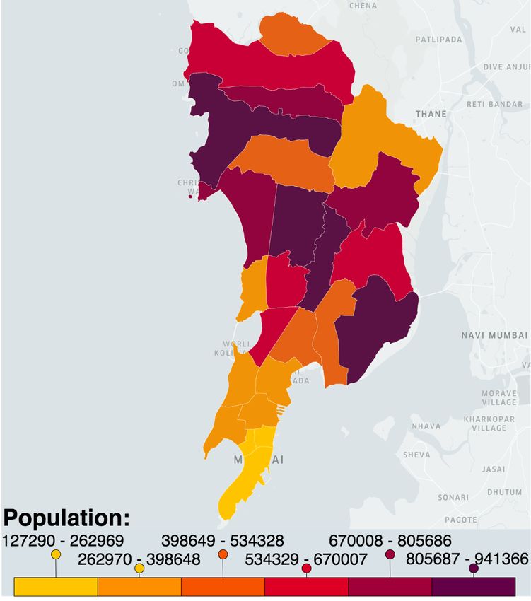
2

lockdown is lifted. More specifically, the post-lockdown scenarios studied, beginning with
the most restrictive, are lockdown for an unlimited period, lockdown until 03 May 2020,
lockdown until 19 April 2020, with various other restrictions either (1) until 31 May 2020,
or (2) until 03 May 2020, or (3) with only case isolation but no other restriction starting from
20 April 2020. In all post-lockdown scenarios, we assume that case isolation will continue
to be active with 90% compliance.
  Our city-scale study suggests that the infection is likely to have a second wave and the
public health threat remains, unless steps are taken to aggressively trace, localise, isolate the
cases, and prevent influx of new infections. The new levels and the peaking times for health
care demand depend on the levels of infection spreads in each city at the time of relaxation of
restrictions. The lockdown has bought us the crucial time needed to do the tracking, isolation,
containment and resource mobilisation.
  Our estimates in this draft are based on an agent-based city-scale simulator, taking a city’s
demographics and interaction spaces into consideration. We use the cities of Bengaluru and
Mumbai as examples, but the study could be extended to other cities as well. The agent-
based simulator includes households, schools/colleges, workplaces, commute-distance based
transport spaces, community spaces, and factors for high density localities. The detailed
modelling of such interaction spaces enables a targeted study of the impact of component in-
terventions and their combinations on the epidemic spread, e.g., schools and colleges closure,
social distancing of the elderly, odd-even strategies, within-city transportation restrictions,
containment zones within the city, etc.
  Our framework could potentially be used to inform testing strategies, but at this time we
have not incorporated them in our study. There is also a potential for mapping vulnerable
zones. We have also not accounted for spontaneous changes in behaviour in the population.
While we have assumed Bengaluru’s and Mumbai’s demographics, the case progression in
hospitals, though age-stratified and adapted to our demographics, is based on available litera-
ture which is still evolving. Availability of more specific case histories from our hospitals will
help us get better estimates of the necessary resources for tackling the epidemic. Instantiations
of the city-scale simulator for multiple cities where the epidemic is prevalent should help us
get better national estimates on the necessary resources for tackling the epidemic.
  We emphasise that this report has been prepared to help researchers and public health
officials understand the effectiveness of social distancing interventions related to COVID-19.
The report should not be used for medical diagnostic, prognostic or treatment purposes or
for guidance on personal travel plans.
3

                              II. U NLOCKING THE LOCKDOWN

  In view of the rising numbers of COVID-19 cases and fatalities in India, the initial 21-
day ‘lockdown’ period which was to end on 14 April 2020 has been extended until 03 May
2020. The website of the Ministry of Health and Family Welfare reported 12289 active cases,
2014 cured/discharged, 488 deaths, and 1 migration, as on 17:00 hrs IST, 18 April 2020. A
few states had already announced an extension of the lockdown prior to the nationwide
extension. Some relaxations are likely after 20 April 2020 based on how the disease spreads
in the coming days.
  The discussion on how to bring about an end to the lockdown needs a systematic study
of the impact of various combinations of non-pharmaceutical interventions. We provide an
agent-based city-scale simulator of an epidemic spread that could be used to inform the
discussion on the easing of restrictions. We hasten to add that our study only looks at public
health outcomes of interventions and their relaxations, and does not consider economic or
ethical issues.
  The simulator helps evaluate scenarios of phased emergence from the lockdown, such as
the following. In all cases, we assume that case isolation (with 90% compliance) remains in
force post the final emergence from lockdown.
  •   A return to normal activity, but with case isolation, on 20 April 2020 as a baseline for
      comparison.
  •   During 20 April 2020 to 03 May 2020, assume case isolation, home quarantine of
      households with cases, closures of schools and colleges, and social distancing of those
      65 years of age or older, with 90% of the household complying. Thereafter, if case
      isolation continues to apply, how does a return to normal activity from 04 May 2020
      (with schools and colleges reopening to complete the term) compare with continued
      closure of schools and colleges until the end of May 2020?
  •   In addition to the aforementioned restrictions from 20 April 2020 to 03 May 2020, add
      an ‘odd-even’ intervention strategy in which only one half of the workforce travels to
      work. Return to normal activity from 04 May 2020, but with case isolation.
  •   Lockdown until 03 May 2020, and return to normal activity on 04 May 2020, but with
      case isolation.
  •   Continue the lockdown for an indefinite period.

  Specific details on the interventions are given in Table I.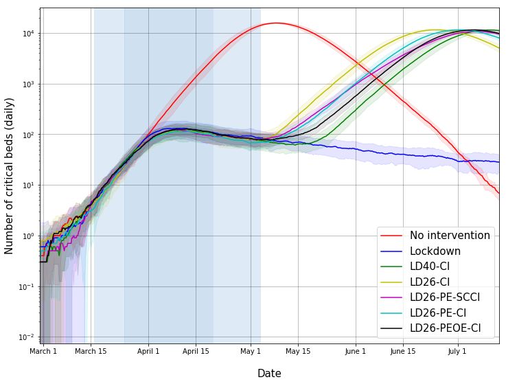
4

                                         TABLE I: Interventions.

 Label       Policy                          Description

 CI          Case isolation at home          Symptomatic individuals stay at home for 7 days, non-household contacts
                                             reduced by 75% during this period, household contacts remain unchanged.
                                             70% of the household comply.
 HQ          Voluntary home quarantine       Once a symptomatic individual has been identified, all members of the
                                             household remain at home for 14 days. Household contact rates double,
                                             contact with community reduce by 75%. 50% of household comply.
 SDO         Social distancing of those      Workplace contacts reduce by 50%, household contacts increase by 25%,
             aged 65 and over                other contacts reduce by 75%. 75% of households comply.
 LD          Lockdown                        Closure of schools and colleges. Only essential workplaces active. For a
                                             compliant household, household contact rate doubles, community contact
                                             rate reduces by 75%, workspace contact rate reduces by 75%. For a non-
                                             compliant household, household contact rate increases by 25%, workspace
                                             contact rate reduces by 75%, and no change to community contact rate.
                                             90% of the household comply with the lockdown.
 LD26-CI     Lockdown for 26 days            Lockdown for 26 days and then normal activity, but with CI. 90% of the
                                             household comply with the lockdown.
 LD40-CI     Lockdown for 40 days            Lockdown for 40 days and then normal activity, but with CI. 90% of the
                                             household comply with the lockdown.
 LD26-PE-    Phased   emergence       (PE)   Lockdown for 26 days, then CI, HQ and SDO for 14 days. Schools and
 CI          from lockdown, scenario 1       colleges remain closed during this period. Normal activity resumes after
                                             this period with reopening of schools and colleges, but with CI. In all
                                             interventions, 90% of the household comply with the lockdown.
 LD26-PE-    Phased   emergence       from   Lockdown for 26 days, then CI, HQ and SDO for 14 days. Schools and
 SCCI        lockdown, scenario 2            colleges remain closed during this period (SC). Normal activity resumes
                                             after this period but schools and colleges remain closed for another 28
                                             days (SC). CI remains in place throughout. In all interventions, 90% of
                                             the household comply with the lockdown.
 LD26-       Phased   emergence       from   Lockdown for 26 days, then CI, HQ and SDO for 14 days. Schools and
 PEOE-CI     lockdown, scenario 3            colleges remain closed and an odd-even workplace strategy is in place
                                             during this period. Normal activity resumes after this period. CI remains
                                             in force throughout. In all interventions, 90% of the household comply
                                             with the lockdown.

  The COVID-19 Community Mobility Report for India [1] in Table II, prepared by Google
based on data from Google Account users who have “opted-in” to location history, indicates
significant reduction in mobility during the lockdown period compared to the baseline period
of 03 January 2020 to 06 February 2020. This informs the nominal contact rate choices in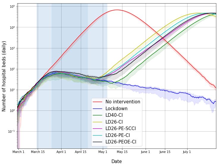
5

Fig. 1: Cases and fatalities all over India (black dots), only in Mumbai (blue dots), and only in Bengaluru
(red dots), in the log scale. Bengaluru data is taken from [2] and Karnataka’s Health and Family Welfare
Department’s media bulletins. Mumbai data is taken from Bombay Municipal Corporation’s Twitter handle.
The first shaded vertical patch shows the lockdown period 25 March - 19 April 2020. The second shaded
vertical patch is the lockdown period 20 April 2020 - 03 May 2020 when some relaxations may be allowed.
The case-to-fatality ratios are different for Mumbai and India. We therefore focus on estimating fatalities.

the interventions’ definitions in Table I.

                TABLE II: Mobility report generated on 11 April 2020, see [1].

                                Place                               Reduction

                                Retail and recreation               -80%
                                Grocery and pharmacy                -55%
                                Parks and public plazas             -52%
                                Public transit stations             -69%
                                Workplaces                          -64%
                                Residential                         +30%

  Simulated outcomes for seven scenarios are given in Figures 2-11 for Mumbai and Ben-
galuru. Some are more likely, others are for baseline comparison. Our study suggests what
might ensue as the infection spreads within one large isolated city. The outcomes are based
on Bengaluru and Mumbai demographic data.
  Figure 1 shows the cumulative number of cases in India, in Mumbai alone, and in Bengaluru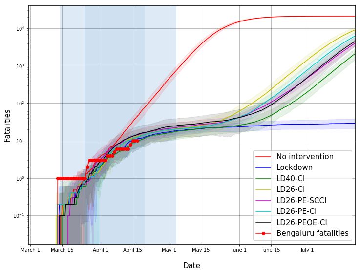
6

alone. The (vertical) offset between the two black curves (in either subpicture) is larger than
the offset between the two blue curves in the top subpicture suggesting a higher case-to-
fatality ratio in Mumbai compared to that all over India1 . There is no evidence to suggest
that the Mumbai infection fatality ratio should be different from the national level. This points
to a combination of under-ascertained cases in Mumbai, or possibly aggressive hospitalisation
elsewhere to facilitate case isolation, or both. We therefore look at reported fatalities to arrive
at our estimates.
      Several significant social distancing measures were already in place prior to the nation-wide
lockdown on 25 March 2020; see Tables III and IV.

                                     TABLE III: Bengaluru timeline, see [4].

             Start date                  Restrictions

             09 March 2020               Closure of kindergartens and primary classes in all schools.
             14 March 2020               Malls, universities and colleges, movie theatres, night clubs, marriages and
                                         conferences and other public areas with high footfall closed.
             16 March 2020               Classes 7 to 9 examinations postponed.
             22 March 2020               Janata curfew. Prohibitory orders until midnight.
             23 March 2020               All nonessential services suspended.
             25 March 2020               National lockdown begins.

                                  TABLE IV: Mumbai timeline, see [5]–[10].

             Start date                  Restrictions

             14 March 2020               Closure of malls, gyms, cinema halls, swimming pools, commercial and
                                         educational establishments.
             15 March 2020               Ban on public gathering and events.
             19 March 2020               Alternate day opening for some close-by pairs of markets.
             20 March 2020               No standing travel allowed in Mumbai’s public transport buses.
             21 March 2020               All workplaces except those providing essential services closed.
             22 March 2020               Janata curfew.
             23 March 2020               District borders closed statewide. Local trains stopped.
             25 March 2020               National lockdown begins.

  1
      Note that we are using this ratio only to compare India levels and Mumbai levels, not for actual estimation of case-to-
fatality ratio. See [3] for issues related to estimation of this ratio.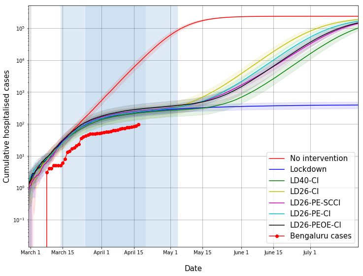
7

  In order to facilitate timely dissemination of our study outcomes, and since we focus
on scenarios post-lockdown, we approximate the effect of these measures as a pre-lockdown
starting 14 March 2020 in Bengaluru and a pre-lockdown starting 16 March 2020 in Mumbai.
  Contact parameters for both Bengaluru and Mumbai were calibrated using smaller scale
replicas (1 million population) of each city. Furthermore, only the growth exponent, or
equivalently the doubling time, of the initial phase of all India COVID-19 fatalities data
was used. See the calibration details in the Methods section of this paper.
  With these assumptions, we get the following estimates for Mumbai and Bengaluru. The
estimates of fatalities refer only to the direct COVID-19 fatalities as a consequence of
the disease mortality and do not include fatalities that are directly or indirectly related to
healthcare capacity limitations.

A. Estimates for Mumbai

  The estimates are in Figures 2-6.
  •   Figure 2: The effect of lockdown on the number of fatalities is seen only around
      14 April 2020 and thereafter. This is consistent with estimated long onset-to-fatality
      duration reported in [3].
  •   Figure 2: Our simulation-based estimate predicts the reduction in the growth rate for
      Mumbai COVID-19 fatalities.
      Figure 3 provides the same estimates of fatalities but in a linear scale for various post-
      lockdown scenarios.
  •   If the lockdown were to continue indefinitely, the number of direct COVID-19 fatalities
      in Mumbai will likely be much smaller than in the no intervention scenario. (In our
      model, assuming 90% compliance, the fatalities reduce to 530 (standard error 190 on
      two Mumbai instantiations with 5 runs on each) compared to 27790 (standard error 210)
      in the no intervention case. These numbers would naturally vary with compliance levels.
      See later pages for Bengaluru estimates.)
  •   If lockdown were lifted on 20 April 2020, and we returned to normal activity, the model
      suggests that the number of direct COVID-19 fatalities may begin to increase, despite
      case isolation, but with some delay. (We assume that cases isolate, but after one day
      following onset of symptoms and only with 90% compliance.)
      As already remarked, this is under the unrealistic assumption that no additional inter-
      vention strategy will be carried out in the interim period.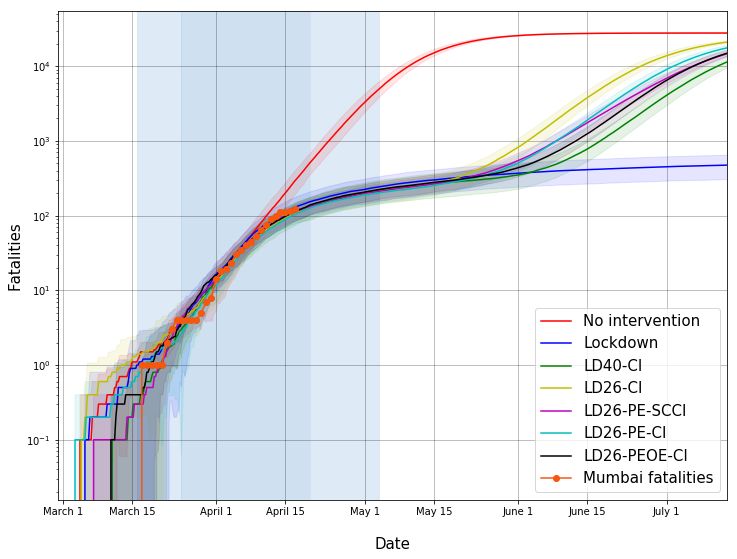
8

  •   If the lockdown is lifted in phases as follows, case isolation plus home quarantine plus
      social distancing of those 65 years and older plus closure of schools and colleges from
      20 April 2020 to 03 May 2020, and thereafter normal activity resumes but with case
      isolation, the direct COVID-19 fatalities may rise once again. This too is under the
      unrealistic assumption that no additional intervention strategy will be carried out in the
      interim period.
  •   While the relaxation of restrictions may result in infection level rising up to near no-
      intervention level, there is yet significant delay before the fatalities start to show an
      exponential growth. This delay may allow better mobilisation of resources for aggressive
      testing, tracking, and containment that can change the course of the epidemic. The
      outcomes of our simulation provide an estimation of this delay.
  •   While the curves for fatalities match the observed data (Figure 2), the number of
      estimated hospitalisations in Figure 4 are off. Possible reasons include a difference in
      Mumbai’s hospitalisation protocol resulting in a later admission to a hospital capable of
      handling COVID-19, or delay on the part of patients in seeking hospital care, or under-
      ascertained cases. These factors must then be adjusted for possible early hospitalisation
      of the actively traced cases to facilitate case isolation. Given these uncertainties, we do
      not attempt to match Mumbai’s cumulative cases curve at this stage, but instead focus
      on fatalities.
  •   Figures 5 and 6: If the lockdown were to continue into the distant future, the peak daily
      demands for regular hospital and ICU beds have likely been reached. We must point out
      that these estimates are based on a disease spread model and hospitalisation protocol
      given in [11] and must be adapted to NCDC/ICMR’s hospitalisation guideline and India
      case histories, once they become available.

B. Estimates for Bengaluru

  .
  Bengaluru has much fewer COVID-19 fatalities than Mumbai and matching to the Ben-
galuru fatality time series is not advisable. To proceed with the estimations, we have assumed
that the Bengaluru cases-to-fatality ratio matches that of India. Under this assumption, we
next provide the estimates for Bengaluru under various post-lockdown scenarios.
  •   If the lockdown were to continue indefinitely, the number of direct COVID-19 fatalities
      in Bengaluru will likely be much smaller than in the no intervention scenario. (In our
      model, assuming 90% compliance, the fatalities reduce to 30 (standard error 10 on two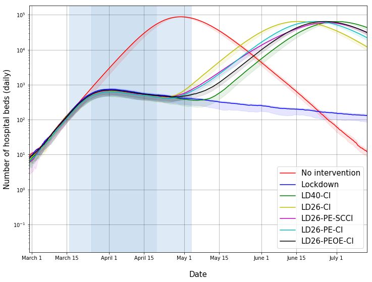
9

Fig. 2: Estimated fatalities in Mumbai in the log scale for various interventions. The first shaded vertical
patch: pre-lockdown period of 16 March 2020 to 24 March 2020. Second shaded vertical patch: lockdown 25

March - 19 April 2020. Third shaded vertical patch: partial lockdown 20 April 2020 - 03 May 2020 when

some relaxations may be allowed. The Mumbai fatalities are based on data gathered from Bombay Municipal

Corporation Twitter Handle. The slowing down of fatalities has been captured by the simulator.

      Bengaluru instantiations with 5 runs on each) compared to 21200 (standard error 120) in
      the no intervention case. These numbers would naturally vary with compliance levels.)
  •   If lockdown were lifted on 20 April 2020, and we returned to normal activity, the
      model suggests that the number of direct COVID-19 fatalities increases to near no-
      intervention level, but with some delay. Again, this is under the unrealistic assumption
      that no additional intervention strategy will be carried out in the interim period.
  •   If the lockdown is lifted in phases as follows, case isolation plus home quarantine plus
      social distancing of those 65 years and older plus closure of schools and colleges from
      20 April 2020 to 03 May 2020, and thereafter normal activity resumes, the fatalities may
      rise once again despite case isolation (one day after symptom onset, 90% compliance.)
      Again, this is under the unrealistic assumption that no additional intervention strategy
      will be carried out in the interim period.
  •   In Figure 9, the cumulative number of hospitalised cases follows the trend in the
      estimates, except for a constant factor offset or delay or both. As already described,
      this might be due to delay in hospitalisation, or delay in seeking hospital care, or due
      to under-ascertained cases.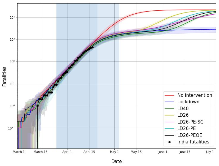
10

Fig. 3: Estimated number of fatalities in Mumbai in the linear scale for various interventions. See details in
caption for Figure 2. A second wave of infection may occur if the first wave is not properly contained.

Fig. 4: Estimated number of hospitalisations (cumulative) in Mumbai. See details in caption for Figure 2. The
estimated numbers are off, perhaps due to hospitalisation modelling assumptions (smaller time to hospitalisation,
delay in seeking hospital care, and under-ascertained cases).

  •   Figures 10 and 11: If the lockdown were to continue into the distant future, the peak daily
      demands for regular hospital beds and ICU beds have likely been reached. We point out
      that these estimates are based on the disease spread model and hospitalisation protocol
      in [11]. The estimate should be adapted to NCDC/ICMR’s hospitalisation guidelines.
11
Fig. 5: Estimated number of hospital beds (daily) in Mumbai. See details in caption for Figure 2. This assumes
a certain case definition for hospitalisation and needs to be refined based on India data. If lockdown continues
far into the future, we have possibly crossed the peak demand point.
Fig. 6: Estimated number of critical care beds (daily) in Mumbai. See details in caption for Figure 2. If
lockdown continues far into the future, we have possibly crossed the peak demand point.
III. E XTENSIONS
The detailed ward-level model can help quantify vulnerabilities of the wards. This can also
help localise the intervention thresholds and strategies. We could have different protocols
for different districts based on “red”, “orange”, and “green” categorisations. The effects of12 Fig. 7: Estimated fatalities in Bengaluru in the log scale for various interventions. The first two shaded vertical patches show the pre-lockdown period of 14 March 2020 to 24 March 2020 and the national lockdown period 25 March - 19 April 2020. The third shaded vertical patch is the lockdown period 20 April 2020 - 03 May 2020 when some relaxations may be allowed. The Bengaluru fatalities are shown as red dots (according to crowd-sourced data in [2], as on 18 April 2020). Fig. 8: Estimated number of fatalities in Bengaluru in the linear scale for various interventions. See details in caption for Figure 7. A second wave may arise if not properly contained now. different zones having different sets of restrictions could be simulated, and one could further study good categorisations of wards into green, orange, and red zones.
13

Fig. 9: Estimated number of hospitalisations (cumulative) in Bengaluru. See details in caption for Figure
7. The estimated numbers are off by a constant factor, possibly due to model assumptions (smaller time to
hospitalisation, delay in seeking hospital care, and under-ascertained cases).

Fig. 10: Estimated number of hospital beds (daily) in Bengaluru. See details in caption for Figure 7. This
assumes a certain case definition for hospitalisation and needs to be refined based on India data. If the lockdown
continues far into the future, we may have crossed the peak demand point.

   One could also study cyclic exit strategies as done in [12]. These should be straightforward
to implement in our simulator.
   With instantiations of a few representative cities, towns, districts, subdistricts, etc., and
14

Fig. 11: Estimated number of critical care beds (daily) in Bengaluru. See details in caption for Figure 7. If
the lockdown continues far into the future, we may have crossed the peak demand point.

with interactions between these entities to model migration and travel, we can patch the
outputs together to obtain nation-wide estimates.
  An additional aspect that could be studied are impacts of hospital bed capacity limitations
and noncompliance. If patients are either asked to go home or are discharged early, with the
advice of home-quarantine, how might this affect the spread in the population? If a fraction of
the population do not comply or if such home-quarantined individuals violate the quarantine,
say for purchasing essential supplies, what might be the consequence? We do not pursue
these questions at this time.

                            IV. M ETHOD : AGENT-BASED M ODELLING

  Our simulator, which enables comparisons such as the above, is an agent-based one that
instantiates a ‘synthetic’ city with various interactions spaces. The synthetic city is matched
to the demographics of a real city, e.g., Bengaluru or Mumbai. We then seed infections and
study how it spreads in the synthetic city under various interventions.
  While SEIR models and even compartmentalised SEIR models with interactions, e.g., [13],
are easy to scale-up, the more detailed agent-based simulators that explicitly bring interaction
15
spaces enable comparisons of various targeted interventions2 .
There are other agent-based simulators that have informed policy decisions3 . Other models
work at an intermediate level by modelling the social network of interactions, e.g., [16].
The purpose of our specific agent-based simulator is to enable comparison of more local
interventions. Since we have explicitly brought out the transport spaces and local community
spaces, our simulator provides an opportunity to compare targeted local strategies, e.g.,
transport spaces operating at half the capacity versus workplaces operating at half the capacity.
Analogous to compartmentalised SEIR models, it would be interesting to ‘patch-up’ multi-
ple city-scale simulators to study the effect of migrations across each component agent-based
simulators. We leave this for later exploration.
The best way to get reliable nation-wide estimates is to have multiple instantiations
representative of big cities, small towns, districts, and subdistricts. We hope our work provides
the impetus to bring to life models of these entities.
The rest of this note describes our simulator.
V. S IMULATOR
A. Agents and interacting entities
We developed an agent-based simulator of an epidemic spread in a city. The model involves
transmission in households, schools and workplaces, community spaces, and transport spaces.
The model uses the following data as input:
• Geo-spatial data that provides information on the wards of a city (components) along
with boundaries. (If this is not available, one could feed in ward centre locations and
ward areas).
• Population in each ward, with break up on those living in high density and low density
areas.
• Age distribution in the population.
• Household size distribution (in high and low density areas) and some information on
the age composition of the houses (e.g., generation gaps, etc.)
• The number of employed individuals in the city.
2
SEIR models capture the average growth patterns. An additional advantage of agent-based models is that they can help
us understand the stochasticity in the disease evolution process, the best case scenarios, the worst-case scenarios, variations
around the mean evolution, confidence intervals, etc.
3
See [11] for UK and USA related studies specific to COVID-19, see [14] and references therein for many agent-based
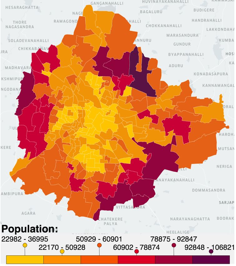
models and their comparisons, and see [15] for a taxonomy.16 • Distribution of the number of students in schools and colleges. • Distribution of the workplace sizes. • Distribution of commute distances. • Origin-destination densities that quantify movement patterns within the city. Taking the above data into account, individuals, households, workplaces, schools, transport spaces, and community spaces are instantiated. Individuals are then assigned to households, workplaces or schools, transport and community spaces. The algorithms for the assignments do a coarse matching. The matching may be refined as better data becomes available. The interaction spaces – households, workplaces or schools, transport and community spaces – reflect different social networks and transmission happens along their edges. There is interaction among these graphs because the nodes are common across the graphs. An individual of school-going age who is exposed to the infection at school may expose others at home. This reflects an interaction between the school graph and the household graph. Similarly other graphs interact. B. Interactions Individuals and households: N individuals are instantiated and ages are sampled according to the age distribution in the population. Households (based on the N and the mean number per household) are then instantiated and assigned a random number of individuals sampled according to the distribution of household sizes. An assignment of individuals to households is then done to match, to the extent possible, the generational structure in typical households. The households are then assigned to wards so that the total number of individuals in the ward is in proportion to population density in the ward, taken from census data. A population den- sity map is given in Figure 12 for Bengaluru and in Figure 13 for Mumbai. The generational gap, household distribution, and age distribution patterns are assumed to be uniform across the wards in the city. Each household in a ward is then assigned a random location in the ward, and all individuals associated with the household are assigned the same geo-location as the household. Based on the age and the unemployment fraction, each individual is either a student or a worker or neither. Assignment of schools: Children of school-going ages 5-14 and a certain fraction of the population aged 15-19 are assigned to schools. These are taken to be students. The remaining fraction of the population aged 15-19 and a certain fraction of the population aged 20-59,
17

                                  Fig. 12: Bengaluru population profile across wards.

based on information on the employed fraction4 , are all classified as workers and are assigned
workplaces. The rest of the population (nonstudent, unemployed) is not assigned to either
schools or workplaces.
      In past works, given the structure of educational institutions elsewhere, educational insti-
tutions have been divided into primary schools, secondary schools, higher secondary schools,
and universities. The norm in Indian urban areas is that schools handle primary to higher
secondary students and then colleges handle undergraduates. We view all such entities as
schools.
      School are located uniformly at random across the city. The number of schools is based on
the number of students and the average school size. We then assign to each school a random
number of students sampled from the school size distribution. Students are then randomly
picked and then assigned randomly to one of the three nearest schools. In the event the
chosen school for a student is already filled to capacity, such students are randomly assigned

  4
      The unemployed fraction in Bengaluru, from the census data, is just over 50%, even after taking into account employment
in the unorganised sector. Similar is the case with Mumbai. This may have some bearing on the epidemic spread.
18
Fig. 13: Mumbai population profile across wards.
to schools with unfilled capacity at the end. This could be updated later based on data of
school locations and travel times to school.
Assignment of workplaces: Workplace interactions can enable the spread of an epidemic.
In principle, Bengaluru’s and Mumbai’s land-use data could be used to locate office spaces.
Two different approaches were taken to assign individuals to workplaces.
In the Bengaluru instantiation, each workplace is located uniformly at random across
the city and is assigned a random workplace size. Distances are then sampled from the
origin-destination intensity data available for the respective cities. For each sampled distance,
individuals whose distances are closest to this value are identified, and one of them chosen
randomly is assigned to this workplace.
In the Mumbai instantiation, data on the number of travelers per day across each ordered
pair of wards (origin-destination matrix of number of travelers) is used to assign individuals
to offices. Based on “zone to zone” travel data from [17] an origin-destination matrix was
extrapolated based on the population of each ward. This origin-destination matrix, for every19 Fig. 14: A simplified model of COVID-19 progression. This can be updated based on data from clinicians and virologists. pair of wards, contains the fraction of employed individuals who belong to the first ward that have offices in the second. The above assignments could be improved further in later versions of this simulator. Community spaces: Community spaces include day care centres, clinics, hospitals, shops, markets, banks, movie halls, marriage halls, malls, eateries, food messes, dining areas and restaurants, public transit entities like bus stops, metro stops, bus termini, train stations, airports, etc. While we hope to return to model a few of the important ones explicitly at a later time, we proceed along the route taken by [18] with two modifications. In our current implementation, each individual sees one community that is personalised to the individual’s location and age and one transport space personalised to the individual’s commute distance. More factors can be brought in at a later time. For ease of implementation, the personalisation of the community space is based on ward-level common local communities and a distance-kernel based weighting. The personalisation of the transport space is based on commute distance. Details are given in Section V-D. Age-stratified interaction: The interactions across these communities could be age-stratified. This may be informed by social networks studies, for e.g., as in [19] which has been used in a recent compartmentalised SEIR model [13]. The output of all the above is our synthetic city on which infection spreads. C. Disease progression We have used a simplified model of COVID-19 progression, based on descriptions in [3] and [11]. This will need updating as we get more information.
20

      An individual may have one of the following states, see Fig. 14:

      susceptible, exposed, infective (pre-symptomatic or asymptomatic), recovered, symptomatic,
hospitalised, critical, or deceased,

      We assume that initially the entire population is susceptible to the infection. Let τ denote
the time at which an individual is exposed to the virus, see Fig. 14. The incubation period
is random with the Gamma distribution of shape 2 and scale 2.29. The mean incubation
period is then 4.58 days (4.6 days in [11] and 4.58 in [20]). Individuals are infectious
for an exponentially distributed period of mean duration 0.5 of a day. We assume that a
third of the patients recover but the remaining two-third develop symptoms. Symptomatic
patients are assumed to be 1.5 times more infectious during the symptomatic period than
during the pre-symptomatic but infective stage. Individuals either recover or move to the
hospital after a random duration that is exponentially distributed with a mean of 5 days5 .
The probability that an individual recovers depends on the individual’s age6 . It is also assumed
that recovered individuals are no longer infective nor susceptible to a second infection. While
hospitalised individuals may continue to be infectious, they are assumed to be sufficiently
isolated, and hence do not further contribute to the spread of the infection. Further progression
of hospitalised individuals to critical care is mainly for assessing the need for hospital beds,
intensive care unit (ICU) beds, critical care equipments, etc. This will need to be adapted to
our local hospital protocol.
      Let us reiterate. Once a susceptible individual has been exposed, the trajectory in Fig. 14
takes over for that individual. Further modulations are (in our current implementation) only
based on the agent’s age.

D. Model of infection spread

      The model of infection spread in such agent-based models is stochastic and utilises the
connection structures already described.
      At each time t, an infection rate λn (t) is computed for each individual n based on the
prevailing conditions. In the time duration ∆t following time t, each susceptible individual
moves to the exposed state with probability 1 − exp{−λn (t) · ∆t}, independently of all other

  5
      This needs to be updated based on hospitalisation guidelines. As discussed earlier, the mismatch in Figure 16 may be
because of either hospital guideline or delay in seeking hospital care or both.
  6
      It is possible to add comorbidities - diabetes, hypertension, etc. - in addition to age. Mortality and prognosis appear to
depend heavily on comorbidities. We leave it for the future.
21
TABLE V: Hospitalisation estimates from [3] while we await reliable data in the Indian
setting.
Age-group % symptomatic cases % hospitalised cases % critical cases
(years) requiring hospitalisation requiring critical care deceased
0 to 9 0.1% 5.0% 40%
10 to 19 0.3% 5.0% 40%
20 to 29 1.2% 5.0% 50%
30 to 39 3.2% 05.0% 50%
40 to 49 4.9% 6.3% 50%
50 to 59 10.2% 12.2% 50%
60 to 69 16.6% 27.4% 50%
70 to 79 24.3% 43.2% 50%
80+ 27.3% 70.9% 50%
events. Other transitions are as per the disease progression described earlier. Time is then
updated to t + ∆t, the conditions are then updated to reflect the new exposures, changes to
infectiousness, hospitalisations, recoveries, etc., during the period t to t + ∆t. The process
outlined at the beginning of this paragraph is repeated until the end of the simulation. ∆t
was taken to be 6 hours in our simulator and is configurable.
A city of N individuals, H households, S schools, W workplaces, one community space
(comprising C wards), one transport space, and associations of individuals to these entities
is the starting point for the infection spread simulator. Infection spread is then implemented
as follows.
An individual n can transmit the virus in the infective (pre-symptomatic or asymptomatic
stage) or in the symptomatic stage. At time t, this is indicated as In (t) = 1 when infective
and otherwise In (t) = 0 otherwise.
Additionally, each individual has two other parameters: a severity variable Cn and a relative
infectiousness variable ρn , see [18]. Both bring in heterogeneity to the model. Severity Cn = 1
if the individual suffers from a severe infection and Cn = 0 otherwise; this is sampled at
50% probability independently of all other events. Infectiousness ρn is a random variable that
is Gamma distributed with shape 0.25 and scale 4 (so the mean is 1). The severity variable
captures severity-related absenteeism at school or workplace, and associated decrease of
infection spread at school or workplace and increase of infection spread at home.
If the individual gets exposed at time τn , a relative infection-stage-related infectiousness
is taken to be κ(t − τn ) at time t. For the disease progression described in the previous22
section, this is 1 in the presymptomatic and asymptomatic stages, 1.5 in the symptomatic,
hospitalised, and critical stages, and 0 in the other stages.
Let βh , βs , βw , βT and βc be the transmission coefficients at home, school, workplace,
transport and community spaces. These can be viewed as scaled contact rates with members
in the household, school, workplace, and community, respectively. More precisely, these are
the expected number of eventful (infection spreading) contact opportunities in each of these
interaction spaces. It accounts for the combined effect of frequency of meetings and the
probability of infection spread during each meeting.
Let nh , ns , nw , nT , nc be the number of individuals assigned to household h, school s,
workplace w, transport space T , and ward c.
A susceptible individual n belongs to home h(n), school s(n), workplace w(n), transport
space T (n) (1 if using public transport and 0 otherwise), and community space c(n).
Interactions without age-stratification: A susceptible individual n sees the following in-
fection rate at time t:
X 1
λn (t) = · In0 (t)βh κ(t − τn0 )ρn0 (1 + Cn0 (ω − 1))
nα
n0 :h(n0 )=h(n) h(n)
X 1
+ · In0 (t)βs κ(t − τn0 )ρn0 (1 + Cn0 (ωψs (t − τn ) − 1))
ns(n)
n0 :s(n0 )=s(n)
X 1
+ · In0 (t)βw κ(t − τn0 )ρn0 (1 + Cn0 (ωψw (t − τn ) − 1))
nw(n)
n0 :w(n0 )=w(n)
!
X dn0 ,w(n0 ) In0 (t)βT κ(t − τn0 )ρn0 (1 + Cn0 (ωψw (t − τn ) − 1))
+ T (n)dn,w(n) P
n0 :T (n0 )=T (n) n0 :T (n0 )=T (n) dn0 ,w(n0 )
ζ(an ) · f (dn,c ) X
+ P f (dc,c0 )hc,c0 (t) (1)
c0 f (dc,c0 ) c0
where
P !
n0 :c(n0 )=c0 f (dn0 ,c(n0 ) ) · In0 (t)βc rc κ(t − τn0 )ρn0 (1 + Cn0 (ω − 1))
hc,c0 (t) = P (2)
n0 f (dn0 ,c(n0 ) )
which will be described soon.
The expression (1) can be viewed as the rate at which the susceptible individual n contracts
the infection at time t. Each of the components on the right-hand side indicates the rate from
home, school, workplace, transport space, and community. The additional quantities, over
and above what we have already described, are as follows.23
The parameter α determines how household transmission rate scales with household size,
a crowding-at-household factor. It increases the propensity to spread the infection by a factor
n1−α . We have taken α = 0.8, see [18].
A common parameter ω indicates how a severely infected person affects a susceptible one,
as will be clear from below. (This is to be tuned at a later stage and is set to 2 now).
The functions ψs (·) and ψw (·) account for absenteeism in case of a severe infection. It
can be time-varying and can depend on school or workplace. We take ψs (t) = 0.1 and
ψw (t) = 0.5 while infective and after one day since infectiousness. School-goers with severe
infection contribute lesser to the infection spread, due to higher absenteeism, than those that
go to workplaces; moreover, the absenteeism results in an increased spreading rate at home.
The function ζ(a) is the relative travel related contact rate of an individual aged a. We
take this to be 0.1, 0.25, 0.5, 0.75, 1, 1, 1, 1, 1, 1, 1, 1, 0.75, 0.5, 0.25, 0.1 for the various
age groups in steps of 5 years, with the last one being the 80+ category.
The quantity hc,c0 (t) represents the transmission rate from individuals in ward c0 to an
individual in ward c. As above, each individual contributes in a distance weighted way in
how individuals in a ward c0 affects an individual in another ward c.
The factor rc stands for a high-density interaction multiplying factor. For Mumbai, rc = 2
for some high density areas and rc = 1 for the other areas. For Bengaluru rc = 1 for all
wards.
The function f (·) is a distance kernel that can be matched to the travel patterns in the city.
Finally, our choice of the infection rate from the community space is a little different from
the rate specified in [18]. However, when the distance kernel is f (d) = 1/(1 + (d/a)b ) and
d
a, i.e., the wards are small, then our specification is close to that indicated in [18]. We
take a = 10.751 km and b = 5.384, based on a fit on data for Bengaluru.
As one can see from (1), we have one community space but with contributions from various
wards. This is to easily amenable to future modifications that include ’containment zones’
and restrict interaction across zones.
Age-stratified interactions: If this is enabled, the home, school, and workspace community
h s w
interaction rates have an extra factor Mn,n 0 , Mn,n0 , and Mn,n0 in the summand which accounts
for age-stratified interactions. Each of these depends on n and n0 only through the ages of
agents n and n0 . The resulting contact rate for individual n at time t is then:24
h
X Mn,n 0
λn (t) = α
· In0 (t)βh κ(t − τn0 )ρn0 (1 + Cn0 (ω − 1))
nh(n)
n0 :h(n0 )=h(n)
s
X Mn,n 0
+ · In0 (t)βs κ(t − τn0 )ρn0 (1 + Cn0 (ωψs (t − τn ) − 1))
ns(n)
n0 :s(n0 )=s(n)
w
X Mn,n 0
+ · In0 (t)βw κ(t − τn0 )ρn0 (1 + Cn0 (ωψw (t − τn ) − 1))
nw(n)
n0 :w(n0 )=w(n)
!
X dn0 ,w(n0 ) In0 (t)βT κ(t − τn0 )ρn0 (1 + Cn0 (ωψw (t − τn ) − 1))
+ T (n)dn,w(n) P
n0 :T (n0 )=T (n) n0 :T (n0 )=T (n) dn0 ,w(n0 )
ζ(an ) · f (dn,c ) X
+ P f (dc,c0 )hc,c0 (t) (3)
c0 f (dc,c0 ) c 0
where hc,c0 (t) is given in (2). Computational complexity can be reduced by focusing only on
the principal components of M h , M s , and M w .
E. Seeding of infection
Two methods of seeding the infection have been implemented.
• A small number of individuals can be set to either exposed, presymptomatic/asymptomatic,
or symptomatic states, at time t = 0, to seed the infection. This can be done randomly
based either on ward-level probabilities, which could be input to the simulator, or it can
be done uniformly at random across all wards in the city.
• A seeding file indicates the average number of individuals who should be seeded on each
day in the first stage of infectiousness (presymptomatic or asymptomatic). This could
be done based on data for patients with a foreign travel history who eventually visited
a hospital. A certain multiplication factor then accounts for the asymptomatic and the
symptomatic individuals that recover without the need to visit the hospital. The seeding
is done at a random time earlier in the time line, based on the disease progression.
F. Interventions and their implementation
The simulator has the capability to accommodate interventions and compliance. Table I
describes some of the interventions in [11], some adapted to suit our demographics, and some
new interventions involving the nation-wide 26-day ‘lockdown’ in India and possible future
scenarios that can bring us out of the lockdown.25
VI. C ALIBRATION
The key parameters to be tuned are βh , βw , βs , βt , βc , and the seeding time prior to some
reference time, 01 March 2020 in our case.
In the current study, although we have a transportation interaction space, we have taken
βt = 0. Bengaluru travel interactions may likely be captured through the local community
interactions. For Mumbai however, local trains are a key mode of daily transportation with
a population of the order of 7.5 million travelling daily using this mode in normal times.
However, trains were stopped in Mumbai prior to the national lockdown and were running
below capacity for at least a week before that. Moreover, the initial infections were seeded
by travellers that came from abroad. The primary mode of travel for this group is unlikely to
be rail transport. So for this version, we have disabled the transport space by setting βt = 0.
Other parameters are the distance kernel parameters, the parameter α that accounts for
crowding in households, the age-stratified interactions, the distribution parameters for indi-
vidual infectiousness, the probability of severity, etc. These are set as follows:
TABLE VI: Model parameters
Parameter Symbol Bengaluru Mumbai
Transmission coefficient at home βh 1.0080 (calibrated) 0.8129 (calibrated)
Transmission coefficient at school βs 1.0164 (calibrated) 1.3019 (calibrated)
Transmission coefficient at workplace βw 0.5082 (calibrated) 0.6509 (calibrated)
Transmission coefficient at community βc 0.2000 (calibrated) 0.1514 (calibrated)
Transmission coefficient at transport space βt 0 0
Household crowding 1−α 0.2 0.2
Community crowding rc 1 2
b
Distance kernel f (d) = 1/(1 + (d/a) ) (a, b) (10.751, 5.384) (4.000, 3.800)
Infectiousness shape (Gamma distributed) (shape,scale) (0.25, 4) (0.25, 4)
Severity probability Pr{Cn = 1} 0.5 0.5
Age stratification Mn,n0 Not used Not used
We assume a counterfactual situation where the current national level of infection is moved
to the city under study. This is clearly not the current situation in India. The COVID-19
epidemic, at this moment, is spread across various cities in India, there are lower levels of
infection in each city and, furthermore, a lockdown is in place. (This gives health officials
an opportunity to aggressively track, localise, and contain the infection.) The counterfactual
situation (all of India’s infections in the isolated city under study) is due to paucity of reliable
city level fatalities data.26
Our simulator was calibrated to match the cumulative case fatalities in India up to 10 April 2020
(199 fatalities) on a synthetic Bengaluru and Mumbai with just one million population. The
India cases and fatalities data is based on daily updates compiled by the European Centre for
Disease Prevention and Control [21]. As mentioned before, the cases-to-fatality ratio seems
to be different for Mumbai and India. So fatalities are likely to be more reliable for tuning
the contact rates. Besides, the fatalities up to 08 April 2020 were likely due to contacts prior
to lockdown. So the effect of lockdown on the calibration is minimised. Also, we consider
a city of size only one million simply for computational ease. Again, in the initial period,
in our modelling framework, once the city is sufficiently large (say, more than 500,000) the
growth of infections and fatalities is more-or-less linear in the city size. In particular, the
parameters that replicate the observed fatalities show negligible sensitivity to the city size
when the city is sufficiently large.
The following tatonnement procedure was used to estimate β values in a no-intervention
scenario. Hundred infected individuals were seeded in the exposed state. The times of their
exposures were sampled according to the Gamma distribution associated with the incubation
period, and the individuals were placed uniformly on the incubation period.
• Based on the estimates in [18], βs was set to twice βw .
• The sizes of βh , βw and βc were then tuned to obtain
– roughly equal transmission probabilities of the disease from home, workplace (schools
and offices), and community;
– a match on the exponential scale of the number of fatalities observed pan-India until
10 April 2020 (199 deaths as per the ECDC numbers).
While the lockdown was already in force from 25 March 2020 to 09 April 2020, the
long mean time to fatality suggests that we may not underestimate the contact rates.
The pan-India numbers were chosen to get a more reliable estimate of the growth
exponent of the number of fatalities. Furthermore, the disease spreads from the immediate
social network neighbourhood of the seeded individuals, with spread in the community
space modulated by distance. The spread will likely be localised in the first few days.
So long as the local neighbourhoods of these networks do not overlap, one could view
the pan-India infections as happening independently in various disjoint localities of
Bengaluru/Mumbai, at least up to a few days post lockdown.
Alternative approaches were also considered, but were abandoned. We identified the num-
ber of individuals who tested positive or were hospitalised (all over India) with a foreign27
travel history. The available information showed that the number of such individuals who
were hospitalised grew exponentially until 24 March 2020 and then decayed exponentially
eventually dropping down to zero. Travel advisory notifications starting from early February,
beginning with visa cancellations of those traveling from China, Korea, Iran, Italy, Japan,
coupled with the long delay from exposure to hospitalisation (mean 10 days in our model)
explain why these numbers fall. However, simulations suggest that using only these as seeds,
with a scale factor for case under-ascertainment, does not explain the continued constant
growth rate in the number of deaths until early April, post lockdown. Perhaps we had entered
the exponential growth phase prior to 24 March 2020. If this were indeed the case, one can
side-step the stochasticity that arises from seeding based on travel histories, and start with
an initial randomly seeded population. This latter approach is what we took to calibrate the
parameters.
The final set of parameters used for the exploration of scenarios are displayed in Table
VI.
For validation, these were then applied to two independently sampled instantiations of Ben-
galuru with population 10 million and two independently sampled instantiations of Mumbai
with population 12.4 million. Five runs were carried out on each instantiation to get the mean
estimates and standard errors of estimates for that city.
Figure 15 matches the number of fatalities in the counterfactual situation used for cali-
bration. Figure 16 shows that estimates of the number of hospitalised cases are off which,
as we explained before, is possibly due to delay in hospitalisation (protocol delay or patient
delay in seeking care) or under-ascertainment.
ACKNOWLEDGMENTS
We sincerely thank G. V. Sagar, Anurag Kumar, Y. Narahari, G. Rangarajan, Vijay Chandru,
Bharadwaj Amrutur, Ramesh Hariharan, Aditya Gopalan, Himanshu Tyagi, Abdul Pinjari,
Navin Kashyap, K. V. S. Hari, Chandra Murthy, Gautam Menon, Jacob John, Prem Mony,
Uma Chandra Mouli Natchu, Mukund Thattai, Siva Athreya, V. Srinivasan, Anil Vullikanti,
Madhav Marathe, Siddhartha Gadgil, Manjunath Krishnapur, Srikanth Iyer, Rahul Lodhe,
Rishi Prajapati, Shipra Jain, Priyanka Agrawal, Subhasis Jethy, Revanth Krishna, Satyajit
Mayor, Rahul Madhavan, Abhijit Awadhiya, Arpit Agarwal, Agrim Sharma, Ashwin M.
S., Shruti Kakade, Micky Kedia, DataMeet (a community of Data Science and Open Data
enthusiasts), Dr. Prabhu, Chiranjib Bhattacharyya, V. Vinay, Avhishek Chatterjee, Abhishek28
Fig. 15: Estimated fatalities in Bengaluru in the log scale for various interventions under the counterfactual
initial condition (all of India’s infections concentrated in Bengaluru). The first shaded vertical patch is the
lockdown period 25 March - 19 April 2020. The second shaded vertical patch is the lockdown period 20 April
2020 - 03 May 2020 when some relaxations may be allowed. The India numbers are shown as blacks dots.
The scenarios are just for additional information and do not include case isolation. The infection rise up once
again after the lockdown period. A similar figure was obtained for Mumbai, but is not included in this draft.
Sinha, Ketan Rajawat, Praneeth Netrapalli, Arpan Chattopadhyay, and other volunteers for
their valuable comments and help.
A PPENDIX A
A RCHITECTURE OF THE IMPLEMENTATION
The following information will be useful for those who wish to download the files and
add their own variations. We will release our code soon.
The workflow is divided into four stages.
1) Data gathering and data preparation for instantiating a synthetic city is the first stage
of the workflow and it involves three sub-stages namely:
(a) Data cleansing and processing: The required data for instantiating a synthetic
city is mined primarily from the decennial census data as well as intermediate
survey estimates for a city. The mined data typically are spreadsheets which are
downloaded in either .xlsx, or .csv file formats. The downloaded files are cleaned
to remove unnecessary columns, null values, duplicates using Python’s pandas29
Fig. 16: Estimated number of hospitalisations (cumulative) in Bengaluru under the counter factual initial
condition. See details in caption for Figure 15. The estimated numbers are off by a constant factor, possibly
due to model assumptions (smaller time to hospitalisation, delay in seeking hospital care, and under-ascertained
cases).
package. The pandas package is further used in data processing which could involve
combining multiple .csv files to obtain the desired input.
(b) Data collation: Required data like demographic information like the total popula-
tion, total number of employed individuals, total number of unemployed individuals
and total number of households for each ward of a city which are extracted from
census tables are processed into .csv files. Further, additional parameters like
the distributions of household sizes, number of students per school and the age
distributions are collated as a JSON file.
(c) Geo-spatial mapping: In addition to the census data, the instantiation for the city
also requires the geographic representations for a ward like the ward centre, ward
boundaries which are obtained from map files. Map files are mined in different
formats like shapefiles (.shp, .shx) or geoJSON (.geojson), which are processed
using Python‘s geopandas package.
2) Instantiating the city files is done by running a python script on the following inputs:
the map data (.geojson), the census data on the demographics(.csv), households(.csv)
and employment(.csv) files along with the additional parameters specified in ‘cityPro-
file.json’. The instantiation of a synthetic city is done in three stages namely:30
(a) Processing Inputs: The script ingests the input (.csv) files using the pandas package
and computes parameters based on the input like the unemployment fraction,
fraction of population in each ward. The GeoJSON file is proceseed with geopandas
pacakge to parses the input file and the shapely package to compute ward centre,
ward boundaries and neighboring wards. Apart from the data files, the target pop-
ulation for which the instantiation is to be done, the average number of students in
a school, the average number of individuals in one workplace are input parameters
specified at the start of the script. The age distribution, household-size distribution
and school-size distribution are taken as inputs from the ‘cityProfile.json’ file.
(b) Instantiating individuals comprises of algorithms which randomly assigns indi-
viduals to households respecting the household-size distribution. Each household
has individuals assigned with generational gaps which respect the age distribution.
Individuals are assigned to workplaces or schools based on their age and assigned
‘workplaceType’ which specifies if the individual is to be assigned a school, a
workflow or neither. Once an individual is assigned to a household, the location
of the individual is mapped to the location of the assigned household. While
instantiating households, the ward number to which the household is assigned
is specified and based on the ward number the respective ward boundaries are
obtained from the map data in the GeoJSON file. The ward boundaries are typically
represented as either ‘Polygons’ or ‘MultiPolygons’. The location of the household
is randomly picked as a point that lies within the polygon. The same logic is used
for instantiating the location of workplaces, and schools. Common areas where
community interactions take place are instantiated at the ward centres, which trans-
lates into finding the centroid of the polygon. These tasks are accomplished using
the following python packages: numpy, random, pandas and shapely. The outputs
of this stage are pandas dataframes for the instantiated individuals, households,
schools, workplaces, transport and community areas.
(c) Additional processing for generating city files: The instantiated dataframes for indi-
viduals, households, schools, workplaces, and common areas are used to generate
the static data files to instantiate the synthetic city. Before generating the city
files, additional processing is done on the dataframes which include computing
the distance of the individuals to their respective ward centres and selecting the
columns that will be used for generating the city files. This stage uses the pandas
package for processing and generating the city files as JSON files where eachYou can also read