Creative Destruction: Barriers to Urban Growth and the Great Boston Fire of 1872
←
→
Page content transcription
If your browser does not render page correctly, please read the page content below
Creative Destruction:
   Barriers to Urban Growth and the Great Boston Fire of 1872∗

                                        Richard Hornbeck
                                  Harvard University and NBER

                                         Daniel Keniston
                                    Yale University and NBER

                                           December 2014

                                              Abstract

          Historical city growth, in the United States and worldwide, has required remark-
      able transformation of outdated durable buildings. Individual reconstruction decisions
      may be inefficient and restrict growth, however, due to externalities and transaction
      costs. This paper analyzes new plot-level data in the aftermath of the Great Boston
      Fire of 1872, estimating substantial economic gains from the created opportunity for
      widespread reconstruction. An important mechanism appears to be positive exter-
      nalities from neighbors’ reconstruction. Strikingly, impacts from this opportunity for
      widespread reconstruction were sufficiently large that increases in land values were
      comparable to the previous value of all buildings burned.

  ∗
     For comments and suggestions, we thank Nava Ashraf, Leah Boustan, Bill Collins, Brad DeLong, Bob
Ellickson, Don Fullerton, Matt Gentzkow, Ed Glaeser, Claudia Goldin, Tim Guinnane, Hugo Hopenhayn,
Matt Kahn, Emir Kamenica, Larry Katz, Michael Kremer, Naomi Lamoreaux, Gary Libecap, Neale Ma-
honey, Sendhil Mullainathan, Derek Neal, Trevor O’Grady, Chris Udry, John Wallis, Bill Wheaton, and
seminar participants at Berkeley, Chicago Booth, EIEF, George Washington, Harvard, Illinois, MIT, NBER,
Northwestern, Pittsburgh, UCLA, and Yale. For financial support, we thank Harvard’s Taubman Center for
State and Local Government and Harvard’s Warburg Fund. For excellent research assistance, we thank Louis
Amira, James Feigenbaum, Jan Kozak, Michael Olijnyk, Joseph Root, Sophie Wang, Alex Weckenman, and
Kevin Wu, in addition to many others for their data entry work.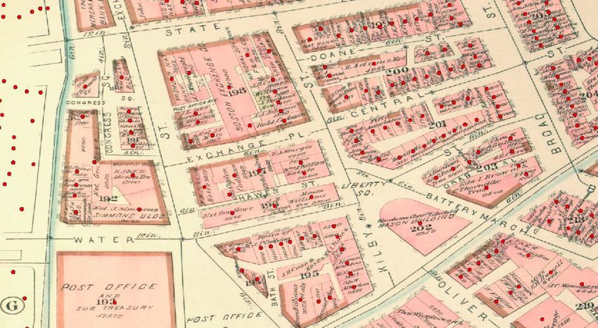
The historical development of the United States has seen a remarkable transformation as
modern metropolises have grown from small cities. Economic growth may strain the capac-
ity of cities to evolve, however, restricting further growth. For example, when landowners’
reconstruction choices do not internalize impacts on neighbors, private replacement of build-
ings diverges from the social optimum. While policy interventions in poor neighborhoods are
widely studied and controversial (Jacobs, 1961; Wilson, 1966; Collins and Shester, 2013), even
wealthy urban areas may not reach their economic potential in the presence of externalities.
Indeed, in the aftermath of the Great Boston Fire of 1872, contemporaries speculated that
this initially calamitous event would generate benefits through the opportunity for major re-
construction (Rosen, 1986), which suggests that substantial frictions in urban growth might
be significantly eased through the opportunity for simultaneous large-scale reconstruction.1
    This paper analyzes the Great Boston Fire of 1872, examining whether the Fire created
real benefits and, if so, through what channels. This historical setting provides an opportu-
nity to observe private landowners’ responses to the opportunity for reconstruction during a
period of urban growth, and avoids challenges of the modern period in which tighter land-
use regulations and government reconstruction efforts often obscure market incentives. The
government had little role in the reconstruction of 1873 Boston, prior to zoning regulations
or stronger building codes in Boston (Rosen, 1986; Fischel, 2004).
    We establish our null hypothesis based upon on a dynamic model of urban growth in
which widespread urban destruction impacts land-use but generates no economic benefits.
In this benchmark case, with no cross-plot externalities from reconstruction, the Fire might
appear partly beneficial because destroyed buildings are replaced with new more valuable
buildings, but the destruction generates no real economic benefits. In the presence of neigh-
borhood externalities, however, reconstruction after the Fire does generate economic gains:
the Fire temporarily improves the equilibrium outcome by forcing simultaneous widespread
reconstruction, which temporarily mitigates the consequences of cross-plot externalities. This
extended model provides a number of testable predictions that we take to the data: increases
in land values in the burned area and nearby unburned areas; increases in building values
in the burned area for even the most high-end buildings, and increases over time in nearby
unburned areas; greater increases in building values following the Great Fire than following
individual building fires; and no increase in land value following individual building fires.
    The empirical analysis uses a new detailed plot-level dataset, covering all plots in the
burned area and surrounding areas in 1867, 1872, 1873, 1882, and 1894. Our digitization
   1
    Throughout the paper we refer to economic inefficiency relative to the efficient economic outcome in
the absence of transaction costs; that is, externalities create an “inefficiency” when transaction costs are
prohibitive for external spillover effects to be internalized.

                                                     1
of city tax assessment records provides data on each plot’s value of land, value of building,
size, owner name, and occupant characteristics. Tax assessment data provide characteristics
for all plots, though a potential concern is whether assessed values accurately reflect market
conditions. We collected supplemental data from Boston’s Registry of Deeds on plot sales,
and show that assessed values align closely with the available sales data in the burned and
unburned areas both before and after the Great Fire.
    We begin by estimating impacts on plots in the burned area, relative to plots in the
unburned area, and then allow the impacts to vary by distance to the burned area. The
identification assumption, that areas would have changed similarly in the absence of the
Fire, is more plausible over shorter periods of time and so we emphasize results in 1873 (and
1882) relative to 1894 (or later periods). While there are differences between the burned
and unburned areas prior to the Fire, contributing to concerns that these areas might have
otherwise changed differently over time, we present empirical specifications that control
for differential levels and trends in pre-Fire plot-level characteristics. We mainly consider
impacts of the Fire on average plot outcomes, supplementing these with quantile regressions
to examine changes in the distribution of outcomes predicted by the model. Using data on
individual building fires that occurred around this period, drawn from Boston fire department
records, we also compare the impacts of individual building fires to the Great Fire.
    The striking initial result is that land values increased substantially from 1872 to 1873
in the burned area, relative to the unburned area. These estimates imply economically sub-
stantial gains from the opportunity for widespread reconstruction, as individual landowners
previously had the opportunity to replace their own building. Land values continued to be
higher through 1882 and, consistent with the model, had reversed by 1894 although the
identification assumption becomes more demanding in later periods. By focusing on plot-
level data within Boston, we analyze the more short-run and medium-run dynamics and the
mechanisms generating economic gains from reconstruction. Initial increases in land value
reflect the creation of economic value, despite subsequent convergence through the gradual
development of other neighborhoods.
    Land values also increased immediately in nearby unburned areas, relative to further
unburned areas. The nearest unburned areas received an increase in land value similar
to the burned area, and the estimated impact declines until leveling at around 1400 feet
(approximately 5-6 blocks or 25-35 buildings away). Given that buildings in the burned area
had hundreds of other buildings within 1400 feet, it is unsurprising that transaction costs
were prohibitive for landowners to internalize spillover impacts. Assuming no impact of the
Fire beyond 1400 feet, the implied total impact on land values is comparable to the total value
of buildings burned in the Fire. Any increase in land value is consistent with economic gains

                                              2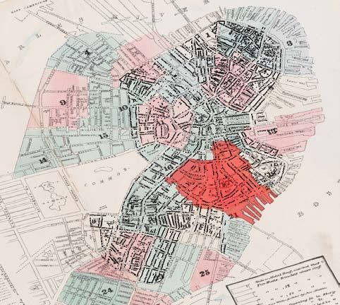
from the Fire, regardless of whether those gains exceed the direct losses from the Fire, but
the value of burned buildings provides a natural benchmark for the economically substantial
magnitude of the impacts. We cannot quantify all spillover effects at the city level, which
might have positive and negative components, but increased land values imply at least large
local gains from the opportunity for urban redevelopment. These relative effects of the Fire,
and in particular the substantial cross-plot spillovers, continue to identify rigidities in urban
growth. Given our estimation of spatial spillover effects, we also note that the statistical
inference is robust to correcting for spatial correlation across plots.
    Building values also increased substantially in the burned area, following reconstruction,
and converged over time. These impacts were greatest at the lowest quantiles of building
values, reflecting replacement of the worst building stock, but building values increased even
at the highest quantiles. Seen through the lens of the model, these results suggest that even
the most recently constructed (and, therefore, the highest value) buildings were replaced
with substantially better buildings, consistent with neighborhood externalities. Likewise, in
nearby unburned areas, estimated increases over time in building values are consistent with
neighborhood spillover effects moving forward the time of optimal building replacement.
    The great extent of the Fire appears central to its impacts, and perhaps the starkest
indication of this phenomenon is seen in the comparison between the Great Fire’s impacts
and the impacts of individual building fires around this period. Building values increased
following single building fires, but building values increased by more following the Great Fire.
Further, while land values increased following the Great Fire, burned plots’ land values were
unchanged following an individual building fire. These estimates are again consistent with
the Great Fire generating some multiplier effect, whether due to neighborhood externalities
or some other mechanism.
    The Fire might also generate economic gains through plot assembly, by discouraging
hold-up and reducing transaction costs. We estimate only small immediate increases in
plot size, however, and these increases are only robust when excluding declines in plot size
from road widening. These changes accompanied a small decline in the number of unique
landowners in the burned area, implying that large landowners did not buy up plots to
coordinate reconstruction on a larger scale. Our interpretation is that the Fire did little to
reduce transaction costs among landowners within a 1400 foot radius, either in coordinating
land assembly or in coordinating building reconstruction, but instead the Fire temporarily
reduced the negative consequences of uncoordinated reconstruction by forcing simultaneous
widespread reconstruction.2 The Appendix reviews these estimates, in addition to exploring
   2
    The continuation of transaction costs, even after the destruction of durable buildings, is consistent with
substantial land rigidities in rural areas (Libecap and Lueck, 2011) and following other urban disasters

                                                      3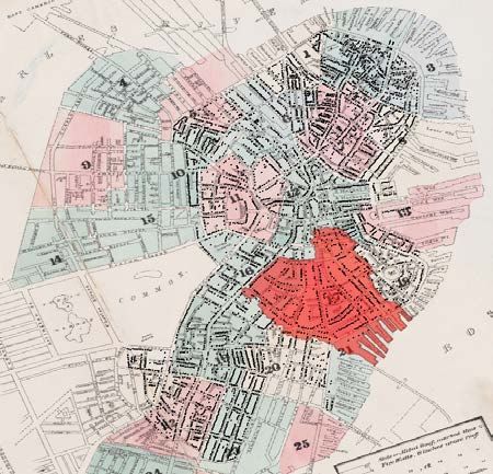
several additional mechanisms through which the Fire might generate economic gains.3
    The Fire itself is not a policy proposal, but the Fire’s impacts are indicative of underlying
economic forces that restrict urban growth.4 Our main interpretation, emphasizing neigh-
borhood externalities, is consistent with research on neighborhood spillovers from urban revi-
talization (Rossi-Hansberg, Sarte and Owen, 2010), rent control (Autor, Palmer and Pathak,
2014), home foreclosures (Campbell, Giglio and Pathak, 2011; Mian, Sufi and Trebbi, 2014),
and gentrification (Guerrieri, Hartley and Hurst, 2013). Policies might correct these exter-
nalities by encouraging large-scale coordinated redevelopment, removing regulatory impedi-
ments to redevelopment, subsidizing individual investments with positive spillovers, and/or
taxing individual investments with negative spillovers. While various policies have been
developed to address similar frictions, including eminent domain, building codes, and zon-
ing regulations, these policies’ application may be ineffective or counterproductive (Munch,
1976; Chen and Yeh, 2013; Turner, Haughwout and van der Klaauw, 2014). Widespread
destruction in the modern era would not generate economic gains if these spillover effects
have been internalized, through regulation or otherwise, but our purpose is to use the Fire
to examine these underlying dynamics in urban growth rather than to estimate the general
impact of destruction itself.
    This historical episode highlights the challenges of maintaining economic growth with
increasingly heterogeneous vintages of capital stock, to such a degree that the destruction
of durable capital generated substantial economic gains. Positive externalities from capital
replacement may be lower in other contexts, due to differences in the economic or policy
environment, but these impacts will be salient in contexts with a return to coordinated
investment. Our focus on a wealthy and growing urban area extends a literature that has
focused largely on the economic impacts of large-scale urban renewal in poor or declining
areas.5 The historical transformation of American cities appears to have occurred despite
(Ellickson, 2013).
   3
     For example, the Fire may have caused changes in the composition of residential and commercial oc-
cupants, which generate spillover effects along with changes in building quality. Similarly, the Fire might
provide an opportunity for industrial firms to change locations and improve the efficiency of their agglom-
eration, though we do not find systematic increases in industrial agglomeration. The Fire also created an
opportunity to improve public infrastructure in the burned area, though there were only moderate changes
in the road network and water pipes.
   4
     Indeed, the implied magnitude of economic loss is larger because even widespread reconstruction after
the Fire is not predicted to obtain first-best land-use in the presence of neighborhood externalities. The Fire
did not decrease cross-building externalities or transaction costs, but temporarily lessened their economic
consequences by spurring widespread reconstruction.
   5
     In our context, it is the growth process itself, combined with the fixed costs of building replacement,
that generates the inefficiencies that are partially alleviated by the opportunity for simultaneous recon-
struction. In our model, areas with declining real estate demand would decline further after widespread
destruction. Particular functional forms for neighborhood externalities could generate multiple equilibria,
however, whereby widespread destruction could generate gains in both declining and growing areas.

                                                      4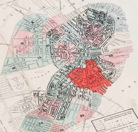
the potential for substantially better economic outcomes, to the point that burning a large
section of Boston generated substantial economic gains in the 19th century.
I       Historical Background
I.A        Great Fires in the United States
Urban fires were a more common occurrence in the 19th and early 20th century United
States than in more recent periods. Dangerous heating and lighting methods led to frequent
small fires amongst densely-located fire-prone buildings (Wermiel, 2000). Individual building
fires exacted a substantial toll and, constrained only by primitive firefighting technologies,
sometimes spread through central business districts completely destroying all buildings in a
wide area.
    Historians and contemporaries generally describe rapid recovery after major city fires,
and even the potential for short-run losses to generate long-run gains (Rosen, 1986). Recon-
struction was primarily managed by the private sector, though governments of burned cities
considered improvements to public infrastructure. Political obstacles largely prevented the
implementation of more ambitious proposals, however, as Rosen (1986) highlights follow-
ing Great Fires in Boston, Chicago, and Baltimore. Following the San Francisco Fire (and
Earthquake), estimates around the burned boundary find increases in residential density
(Siodla, 2013) and firm relocation (Siodla, 2014).
I.B        The 1872 Great Fire of Boston
In November 1872, a small fire spread through a large section of Boston’s business district,
eventually destroying 776 buildings over 65 acres of the downtown Boston area (Figure
1).6 Boston firefighters were unable to stop the fire before it spread, due partly to sickness
amongst the fire department’s horses that prevented the rapid deployment of equipment to
the burning area (Fire Commission, 1873). The Fire burned for 22 hours, eventually stopping
with the arrival of massive firefighting resources from surrounding areas. The Fire killed 20
people and caused approximately $75 million in damages, or 11% of the total assessed value
of all Boston real estate and personal property (Frothingham, 1873).
    In anticipation of the empirical analysis, a natural question concerns the endogeneity of
which plots burned. The Fire began in the south-central part of the burned region and spread
out and to the North, toward somewhat more valuable parts of the downtown area. Extensive
investigations and hearings following the Fire provide no accounts of the fire department
protecting areas differentially, which were all fairly high value at the time (Fire Commission,
1873; Fowler, 1873). Wide roads provided a natural barrier to the fire spreading, though the
    6
        Figure 1 also shows the location of individual land plots in our main sample, which we discuss below.

                                                        5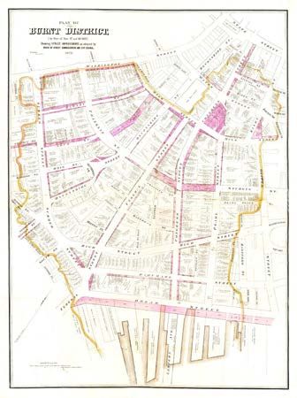
Fire sometimes crossed wide roads and sometimes ended within a block.7 In practice, the
empirical analysis will include controls for pre-Fire plot outcomes that allow for differential
changes over subsequent periods.
    In anticipation of the theoretical framework, we note that the Fire occurred following
a period of growth in Boston real estate values (Appendix Figure 1). Boston real estate
values declined in real terms later in the 1870’s, during the national “Long Depression,” but
subsequently resumed their upward growth.8
    The Fire prompted substantial inflows of private sector capital to fund reconstruction,
given the strong demand for real estate investment in Boston. Boston capital markets were
well-integrated at this time, both domestically and internationally, so we assume perfect
capital markets in the model. Insurance payouts also partly funded reconstruction.9 Insur-
ance payouts should not impact optimal land-use in the presence of perfect capital markets,
though we do explore in the empirical analysis whether landowners disproportionately exited
the burned area.10
    Individual landowners retained their land rights after the Fire, and reconstruction was
largely managed privately. Although the weeks immediately after the Fire saw calls for
government action to coordinate reconstruction, the ultimate role of the city government
in post-fire reconstruction was limited. The city purchased some land to widen and extend
downtown roads, though landowners’ opposition stopped more-ambitious proposals to modify
the road network. Similarly, calls for a strong building code were undermined, and the
ultimate legislation was weak and substantially rescinded in 1873 (Rosen, 1986).
    Newspapers and other contemporaries noted that buildings in the burned area were
often better after reconstruction. On the one year anniversary of the Fire, the Evening
Transcript concluded that the “improved aspect of the entire district shows that occurrences
calamitous in their first effects sometimes result in important material good” (Rosen, 1986).
Technological constraints precluded the reconstruction of taller buildings, and there had been
no substantial recent changes in construction technologies, but buildings could be improved
along more subtle dimensions (Rosen, 1986).11
   7
      We do not observe systematic differences in 1872 in land value and building value across the Fire
boundary, using our data and restricting the sample to plots within 100 feet of the Fire boundary.
    8
      We convert valuations to constant 1872 dollars using the David-Solar CPI (Lindert and Sutch, 2006).
    9
      Insurance covered three-fourths of total fire damages, though many insurance companies were bankrupted
by the Fire and payouts were roughly half of total damages (Fowler, 1873).
   10
      In practice, some landowners may have been liquidity-constrained after the fire destroyed their property
and the collateral needed to raise more capital. We would have been interested in testing this hypothesis
more fully, though we have been unable to link particular plots to their insurance underwriter and the
fraction paid out on the insurance policies.
   11
      Qualitative accounts also include descriptions of the Fire encouraging the assembly of land into larger
plots (Rosen, 1986).

                                                      6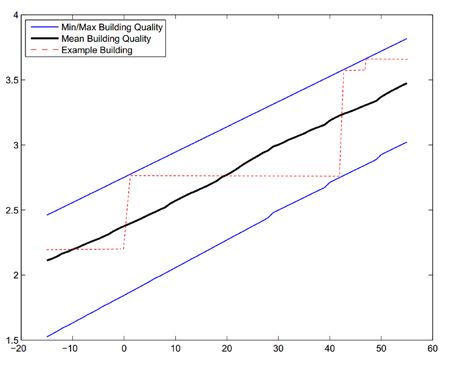
Even substantial upgrading of buildings need not imply any economic gains from the
Fire, however, and we formalize this intuition below in our benchmark model. We then
present an extended model with neighborhood externalities, which highlights how the Fire
might indeed result in important material good.
II     Dynamic Model of Urban Growth
II.A     Benchmark Model with Durable Buildings
Our benchmark model clarifies conditions under which the Fire may only appear to generate
economic benefits. We consider the decisions of landowners choosing when to replace their
building, but who experience no spillover impacts from nearby plots. This benchmark model
formalizes our null hypothesis, in which the Fire does not generate any economic benefits.
The benchmark model and the extended model yield dynamics similar to one-sided s-S
models of price-setting and vintage capital replacement, and generate a number of testable
predictions that we take to the data.
    We assume that each landowner owns one plot, and that all landowners and plots are
homogeneous. Landowners construct a sequence of durable buildings to maximize the net
present value of rents from their plot, which are assumed to depend solely on the quality
of their building (q) and the city’s overall productivity (ωt ). In each period, a building of
physical quality q generates rent of r (q, ωt ). In particular, we assume that the marginal
return to building quality is increasing in city productivity: ∂ 2 r (q, ωt ) /∂q∂ωt > 0. We
adopt a broad view of city productivity, which simply reflects aggregate market conditions
that influence building rents.
    We focus on the case in which city productivity is growing over time, which increases the
return to building quality and encourages landowners to construct higher quality buildings.
The predicted impacts of a Great Fire would differ in a city with declining productivity.12
    For clarity, we assume that landowners may only completely replace their old building
                                  0                                0
with a new building of quality q by paying a convex cost c q .13 In particular, we as-
sume that buildings cannot be renovated and that buildings do not depreciate. These two
assumptions make the model’s predictions more apparent, but do not qualitatively change
the predictions.14 As a matter of notation, we assume that building construction is instan-
  12
     Notably, the failure of declining cities to recover after disasters is not inconsistent with our predictions;
indeed, we would predict that widespread destruction would hasten the decline of cities otherwise declining.
Only in cities in which developers believe that returns to real estate investment will rise in the future would
we predict that destruction generates increased building quality.
  13
     The assumption of convex costs guarantees an interior solution.
  14
     The model’s qualitative predictions are robust to the introduction of building depreciation or partial
renovation, as long as the cost of renovating to the optimal quality ultimately becomes greater than the
costs of constructing a new building of the desired quality.

                                                        7
taneous.15 We also assume there are no demolition costs.16
Building construction is a forward-looking dynamic optimization problem, in which each
landowner considers the optimal time to replace a building. Landowners do not replace a
building when it would generate higher static rents; rather, landowners solve for the optimal
replacement policy incorporating the option value of retaining antiquated but still profitable
buildings. This intuition is captured by the following Bellman equation, which reflects the
landowner’s value of owning a building of quality q when the city has productivity ωt (and
includes the option to rebuild):
(
r (q, ω) + δE [V (q, ω 0 )]
V (q, ω) = max
r (q ∗ , ω) + δE [V (q ∗ , ω 0 )] − c (q ∗ )
where q ∗ maximizes r (q, ωt ) + δE [V (q, ω 0 )] − c (q). That is, q ∗ represents the optimal qual-
ity building to construct if the landowner chooses to construct a new building. Buildings
face a probability d of experiencing an idiosyncratic fire that forces their owners to rebuild
completely in the next period. Owners’ expectations of future valuations are thus
E [V (q, ω 0 )] = (1 − d) V (q, ω 0 ) + d · V (0, ω 0 )
with q = q ∗ if the building has been reconstructed that period.
The landowner faces a tradeoff between two choices: (1) receiving rent r (q, ωt ) and
continuing with the old building of quality q; and (2) paying a lump sum cost c (q ∗ ) to
construct a higher-quality building, receiving higher rents, and continuing with the new
building of quality q ∗ . The random destruction of buildings, with some probability d, provides
a mechanism to consider the impacts of an individual building fire. Notably, in this case of
exogenous building destruction between periods, the landowner will choose to rebuild in the
next period at quality q ∗ .
Landowners’ optimal construction decisions involve periods of no activity and occasional
quality upgrades, consistent with the equilibrium in one-sided s-S models. Given that city
productivity is increasing, landowners over-build for contemporaneous conditions and then
wait for city productivity to increase before replacing their then-obsolete building. To illus-
trate the equilibrium building growth paths, we assume r (q, ω) takes the Cobb-Douglas form
q α ω β (α ≥ 0, β ≥ 0, α + β ≤ 1), with c (q) = cq γ (c > 0, γ > 1).17 We generate a sample
15
Equivalently, foregone rents could be included in the cost of construction.
16
Demolition costs could be included in the cost of construction, as a fixed cost component. Fire might
reduce some portion of demolition costs, but these costs then become sunk and do not influence subsequent
construction decisions or become capitalized into building value or land value.
17
In our quantitative simulations we set δ = 0.9, α = β = .5, γ = 2, and c = 5. The probability of
8of 3000 buildings and simulate the model until it reaches steady-state, i.e., until the growth
rate of the distribution of buildings stabilizes.
Figure 2, Panel A, graphs the steady-state evolution of the building distribution. The
thick central line shows the mean of log building quality, which grows at a constant rate in
steady state driven by the constant growth in city productivity. There are discrete jumps,
however, in the growth paths of individual buildings. Newly constructed buildings are the
highest quality buildings for one period, before being surpassed by more-recently constructed
buildings. The upper thin line denotes the maximum of log building quality in steady state,
which reflects the optimal building to construct when constructing a new building in that
period (whether by choice or because the building was exogenously destroyed).18 Surviving
buildings are endogenously replaced once city productivity increases sufficiently, and this
minimum threshold in log building quality is represented by the lower thin line.
One example building growth path, shown as a dashed line in Panel A, reflects periods
of endogenous reconstruction and exogenous destruction. In period 0, the building is exoge-
nously destroyed and is reconstructed at a higher quality level. The building remains at this
quality level as city productivity grows, until in period 42 the landowner finds it optimal to
finally tear down the building and replace it with a substantially higher quality building.
This building happens to be exogenously destroyed a few periods later, and is rebuilt to only
slightly higher quality.
Figure 2, Panel B, graphs the steady-state evolution of the building distribution for a city
that experiences a “Great Fire” in period 0 that destroys half of the buildings. Outcomes for
the burned buildings are shown using dashed lines, and outcomes for the unburned buildings
are shown using solid lines. The Fire induces all landowners in the burned area to reconstruct
their building at the current optimal quality, which raises average building quality. Further,
the Fire compresses the distribution of building qualities in the burned area around the
maximum: burned buildings are rebuilt to the same quality as newly reconstructed buildings
in unburned areas, such that there is no impact at the highest quantiles of the distribution
of building values.19 The Fire’s impacts on building quality are greatest toward the bottom
of the distribution, where the entire stock of older buildings is cleared out.
In this benchmark model, the Fire does not affect landowners in unburned areas. Over
time, landowners in unburned areas choose to replace their buildings and landowners in
the burned area delay further replacement, such that the distributions of building quality
exogenous destruction (d) is set to 0.01, and the growth rate is set to 0.06.
18
Note that the optimal new building is “over-built,” as its quality is higher than the optimal quality if
there were no expected future growth in city productivity.
19
We assume the Fire does not directly raise construction costs temporarily, which might otherwise impact
reconstructed building values or delay reconstruction.
9converge. Notably, convergence is slower for the bottom of the distributions. As a result,
the average quality of unburned buildings will surpass the average quality of rebuilt burned
buildings for some periods and then oscillate until random building destruction induces long-
run convergence.20
While the burned area might appear more-developed shortly after the Fire, there are
no economic gains from the Fire in this benchmark model. All landowners could choose
to replace their buildings in period 0 in the absence of the Fire, but the large majority of
landowners instead prefer to postpone reconstruction. There would be economic gains from
forcing individual landowners to reconstruct buildings if there were positive externalities
from reconstruction, however, which we explore in the next section.
This benchmark model yields five main testable predictions. First, the Fire does not
increase plot land values, which reflect the option value from each land plot, V (0, ωt ). Sec-
ond, the Fire increases average building values in the burned area, following reconstruction,
which then converge to average building values in unburned areas. Third, the Fire’s impact
on building values is decreasing in the quantile of building value, and is zero at the highest
quantiles. Fourth, the Fire has the same impact on building values as individual building
fires. Fifth, building values and land values are unaffected in unburned areas.
II.B Extended Model with Neighborhood Externalities
We now extend the benchmark model, allowing for building rents to increase in the quality
of nearby buildings. These spillover effects generate externalities, given assumptions that
land ownership is fractured and transaction costs are prohibitive to coordinate construction
decisions. In this extended model, the Fire generates economic gains that may partially or
fully offset the direct losses from destruction.
Consider a modified building rent function of r (q, Q, ωt ), where Q is a vector of nearby
buildings’ qualities with mean Q̄. We assume that the number of surrounding buildings is
sufficiently large that landowners take Q as given, such that neighborhood spillovers repre-
sent a pure externality. In particular, higher building quality generates positive externalities,
as building rents are increasing in the quality of nearby buildings (∂r (q, Q, wt ) /∂ Q̄ > 0).
Further, the return to building quality is increasing in the quality of nearby buildings
(∂ 2 r (q, Q, wt ) /∂q∂ Q̄ > 0).21 We can adopt a broad view of “neighborhood quality,” and the
channels through which building rent is impacted by nearby plots. We have no strong prior
20
The model generates a sharp reversal, as landowners in the burned area choose to replace a large
number of surviving buildings reconstructed after the Fire, though this dynamic would be smoother with
some random shocks to the incentives for reconstruction.
21
The first assumption causes widespread reconstruction to generate economic gains for landowners,
whereas the second assumption generates a multiplier effect in which simultaneous reconstruction encourages
even higher-quality reconstruction of burned buildings (and nearby unburned buildings).
10regarding which buildings are sufficiently “nearby” to influence building rents, but make an
assumption for the numerical simulation below and later estimate these spillover effects.
The landowner’s value of owning a building of quality q when the city has productivity
ωt is now given by:
(
r (q, Q, ωt ) + δE [V (q, Q0 , p0 )]
V (q, Q, ωt ) = max
r (q ∗ , Q, ωt ) + δE [V (q ∗ , Q0 , p0 )] − c (q ∗ )
where q ∗ maximizes r (q, Q, ωt )+δE [V (q, Q0 , p0 )]−c (q) and the vector Q reflects the building
quality decisions of nearby landowners.
An individual building fire continues to have the same impacts as in the benchmark model.
Following an individual building fire, with no change to the quality of nearby buildings, the
burned building is reconstructed to quality q ∗ .22
The Great Fire, however, creates a positive multiplier effect because owners of burned
properties take into consideration the simultaneous construction of many surrounding higher-
quality buildings. This encourages even higher building qualities due to the assumption of
complementarity, and higher overall rents due to the assumption of positive neighborhood
spillovers. In nearby unburned areas, landowners benefit from higher building qualities in the
burned area and some landowners choose to upgrade buildings earlier. Over time, landowners
in further unburned areas also choose to reconstruct their buildings sooner and to a higher
quality level due to increases in nearby buildings’ quality. In this manner, the impacts of a
Great Fire spread through the city.
Landowners’ construction decisions are not efficient after the Fire, as the spillover effects
are still not internalized by landowners, but the Fire temporarily reduces the inefficiency.
Prior to the Fire, there is a disperse distribution of building qualities that includes some
older, low-quality buildings. Since landowners consider the whole distribution of neighbors
when reconstructing properties, new buildings are lower quality than if all other buildings
were also replaced. The Fire transforms this sequential game into a simultaneous game, and
in a growing city landowners construct buildings of yet higher quality.
We focus on a single equilibrium case, in which decreasing returns to quality cause the
Fire’s impacts to fade over time as city productivity increases and all buildings are replaced.
Indeed, in some later periods, burned areas are relatively disadvantaged because of the large
concentration of then-obsolete buildings constructed in the immediate aftermath of the Fire.
22
We assume that one building makes a trivial contribution to the overall vector of neighborhood buildings.
In principle, the earlier-than-expected reconstruction of that one burned building has some small unexpected
benefit to nearby landowners and encourages them to reconstruct their buildings sooner. This small increase
in the expected future quality of neighboring buildings would encourage the burned building to be rebuilt
to slightly higher quality.
11By contrast, for other particular functional forms of neighborhood spillovers, the Fire could
have persistent impacts due to multiple equilibria.
To illustrate the effects of the Fire, we extend the numerical simulation to include neigh-
borhood spillover effects. We modify the rent function, dividing the productivity term into
the effect of city-wide productivity (ωt ) and the impact of neighborhood building quality
β
(Q) : r (q, Q, ω) = q α (Qη ω 1−η ) .23 We assume that the average quality of neighboring
buildings
P summarizes
the spillover effects from neighbors: if building i has N neighbors,
N
Qi = n=1 qn /N . Otherwise, the simulation is the same as for the benchmark model. In
the steady state, there is a constant rate of growth in neighborhood productivity (Qη ω 1−η ).24
Figure 3, Panel A, shows the changes in building quality after a Great Fire for burned
buildings whose “nearby” buildings all burn. Dashed lines show changes for the burned plots,
and solid lines represent changes had there been no Fire. The presence of value spillovers
creates a multiplier effect from simultaneous reconstruction that causes buildings’ quality in
the burned area to rise temporarily above that of the best buildings had there been no Fire.
The Fire’s impacts are again greatest toward the bottom of the distribution but, in contrast
to the baseline model, continue to positively impact values at even the highest quantiles.
Note that these effects would not apply to an individual building fire, where the milder
predictions of the baseline model continue to hold. Over time, as in the benchmark model,
building quality converges with oscillation to the same steady state had there been no Fire.
The Fire now affects landowners in unburned areas that are close enough to the Fire to
experience changes in Q due to post-Fire reconstruction. Figure 3, Panel B, shows the growth
path for unburned areas for whom half of their “nearby” buildings burned, and the solid
lines continue to represent changes had there been no Fire.25 The Fire causes landowners in
nearby unburned areas to upgrade their buildings sooner, due to reconstructed higher-quality
buildings in the burned area.26 These geographic spillover effects within the city complicate
an analysis of the Fire’s aggregate impacts, as even the comparison group is affected by the
treatment, and we return to this issue in the empirical analysis.
Predicted impacts on land values are of particular interest. In the model, a natural
23
In our simulation, we set η = 0.8 (and continue to set α = β = 0.5).
24
One technical challenge concerns owners’ beliefs about the transitional dynamics immediately after the
Fire. For simplicity, we assume that owners expect productivity and neighboring building quality to grow
at the same rate after the Fire as prior to the Fire. These beliefs are correct in the long-run, and the main
numerical results are not sensitive to alternative beliefs during this period of transition. In particular, model
predictions are qualitatively robust to the opposite, and overly pessimistic, assumption that neighboring
building quality will cease to grow entirely after the Fire.
25
In particular, we simulate a nearby unburned area in which plots receive 1/2 the Q̄ spillovers of plots
with all burned neighbors.
26
In practice, if the Fire were to temporarily raise construction costs, then we might expect reconstruction
of nearby unburned buildings to be delayed until after the burned area is reconstructed.
12definition of land value is the option value from owning a plot with no building: V (0, wt ).27
There is no distribution of land values because plots are homogeneous, so we show changes
in the value of land for each plot. Figure 4 shows the value of land in the benchmark model
where the Fire has no impact on land value (lower black line). For the extended model
with neighborhood spillovers, the upper red line shows increased land values in the burned
area. The middle blue line shows smaller increases in land value for nearby unburned areas
receiving spillovers from neighboring burned areas as described above.
The extended model with neighborhood externalities yields seven main testable predic-
tions, of which five differ from predictions of the benchmark model. First, the Fire increases
plot land values in the burned area and land values converge over time, perhaps even falling
below land values in unburned areas. Second, the Fire increases land values in nearby un-
burned areas. Third, as in the benchmark model, the Fire increases average building values
in the burned area, following reconstruction, which then converge to average building values
in unburned areas. Fourth, the Fire’s impact on building values is decreasing in the quantile
of building value, as in the benchmark model, but there are temporary impacts at the highest
quantiles. Fifth, the Fire increases building values in nearby unburned areas. Sixth, the Fire
has a greater impact on building values than individual building fires. Seventh, as in the
benchmark model, individual building fires have no impact on land values.
II.C Additional Potential Mechanisms
There are several additional channels through which a Great Fire might impact urban growth.
We discuss some of these channels below, and present some empirical analysis of these
channels in the Appendix.
Land Assembly and Ownership Concentration. We have assumed that post-Fire redevel-
opment occurs within fixed land plots, though the Fire might have impacts through land
assembly. Land assembly, or the combination of plots, allows the construction of larger
buildings and might create more value per-unit of land when there are otherwise rigidities
preventing land assembly (see, e.g., Brooks and Lutz, 2012).
There are two main reasons why the Fire might increase plot sizes in the burned area.
First, the Fire might reduce transaction costs resulting from hold-up or other aspects of
bargaining between plot buyers and sellers.28 Second, local heterogeneity in building quality
27
Note that this value equals the value of owning a building of quality q that would be chosen for replace-
ment (i.e., a “tear down” building): V (0, wt ) = V q, wt .
28
The bargaining power of some landowners may decline after a fire: their outside option has worsened
because they cannot live in the building or continue to operate a business without substantial reconstruction
costs, and some may lack liquidity and become impatient (e.g., if they are less-wealthy or less-diversified).
The Fire also reduces imperfect information about the value of burned plots, as there is no uncertainty
regarding building value.
13may discourage otherwise profitable plot consolidation even within a single owner’s neigh-
boring holdings.29 By destroying all buildings in an area, the Fire coordinates the timing
of new construction and lowers the cost of land assembly. The Fire might also concentrate
land ownership, thereby improving the coordination of urban development.
Business Agglomeration. The Fire may also impact urban development by improving
the efficiency of firms’ location decisions. Whereas firms generally make sequential location
decisions, the Fire may allow firms to move simultaneously into a more-productive spatial
distribution. Firms have many reasons to locate near similar firms or firms producing inputs
or complementary goods.30 The size and location of industrial clusters may drift from the
optimum over time, however, as the city develops and new technologies are introduced. The
Fire might increase industrial agglomeration, or otherwise improve the efficiency of firm
locations, by reducing moving costs and improving cross-firm coordination.
Occupant Sorting. Similarly, the Fire might impact residential or industrial sorting along
with replacement of the building capital stock (see, e.g., Brueckner and Rosenthal, 2009). If
occupant characteristics generate spillover effects, and occupants’ location is fairly persistent,
then these spillover effects could become capitalized into land values and influence land-use.
In general, if occupant characteristics are correlated with building characteristics then we
would consider building spillover effects to come from some potential combination of the
two. Changes in occupant characteristics provide an additional mechanism through which
building reconstruction generates spillover effects.
Infrastructure Investment. The Fire may create a unique opportunity for improvements
in roads and other infrastructure. First, the absence of buildings lowers the costs of land
acquisition and construction. Second, post-disaster solidarity may strengthen political will
for public goods improvements.
III Data Construction
III.A Annual Tax Assessment Records
Historically, the City of Boston sent tax assessors to each building to collect information
for annual real estate and personal property taxes. The Boston Archives contain these
handwritten ledgers from 1822 to 1944, typed records until 1974, and then digitized data.
Tax assessors recorded information for each building unit, each commercial establish-
ment, and each residential occupant. For each building unit, data include: street name and
number, assessed value of the building, assessed value of the land, plot size, and name of
29
When reconstructing an older building, the nearby newer buildings may be prohibitively costly to tear
down early to build one larger building.
30
Optimal industry locations can reduce transportation costs, attract customers interested in cross-
shopping, signal competitive prices, allow monitoring of competitors, or encourage learning.
14the building owner. For each commercial occupant, data include: detailed industry, value
of business capital, and proprietor name. For each residential occupant, data include the
value of personal possessions and the name and occupation of all males aged 20 or older.
We collected all of these variables, aside from commercial proprietors’ names and residential
occupants names and occupation.31 We digitized data for 1867, 1872, 1873, 1882, and 1894,
covering all plots in the area burned during the 1872 Fire (which occurred after that year’s
tax assessment) and all plots in surrounding downtown areas.32
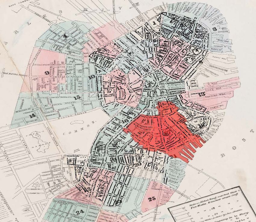
III.B Plot-Level City Maps
The assessment data contain addresses, but these addresses do not directly provide plots’
geographical proximity to the Fire. We generated this measure by plotting each assessment
entry on high resolution scans of the plot-level Sanborn and Bromely fire insurance maps of
Boston in 1867, 1873, 1883, and 1895 (Sanborn Map Company, 1867-1895; G.W. Bromley
and Co, 1883). These maps indicate the location of each building and its street address
(Appendix Figure 2), and often indicate the plot’s square footage and owner name, which
were used in matching the assessed plots to their geographic location. We georeferenced these
historical maps to a contemporary digital map of Boston, defining each map in geographic
space. Figure 1 maps the location of digitized land plots in 1867, and we limit the sample
to land plots in this same region in each subsequent year (Appendix Figure 3). There are
31,000 land plots in our main sample, pooling across all five years.33
The empirical analysis benefits in a number of ways from assigning the geographic location
of each plot. First, we can calculate whether each plot is in the burned area and its distance
from the burned area. Second, we can effectively analyze a panel dataset of fixed geographic
locations despite potential changes over time in street addresses and plot boundaries. Third,
we can match plots to their pre-Fire outcomes by city block or match plots to their nearest
corresponding plot prior to the Fire, which allows the empirical specifications to control
for differential changes associated with pre-Fire differences. Fourth, and similarly, we can
31
We collected commercial proprietors’ industry, but did not collect residents’ occupation because the
land itself is used for housing and our analysis is focused on land-use. We also did not collect the names
of commercial proprietors and residential occupants, as we would not be able to track individuals moving
in/out of the neighborhoods analyzed and names are relatively costly to digitize.
32
Through selective double-entry and back-checks, we have found initial entry and data cleaning to pro-
duce highly accurate data. Tax assessors totaled the numeric data at the bottom of each page (capital,
possessions, land value, building value, plot size), which was used to validate the sum of entered data. The
data include what are now the West End, North End, Financial District, Downtown Crossing, Leather Dis-
trict, Chinatown, and Fort Point. The data exclude more residential areas in what are now the South End,
Back Bay, and Beacon Hill.
33
We exclude wharfs, which are incompatible with the model in that the land area itself is endogenous.
The estimated impacts on land and building value are similar, or somewhat higher, when including plots
from wharfs.
15calculate each plot’s distance to the Old State House, as a proxy for the center of the central
business district, and control for differential changes associated with this distance. Indeed,
in principle, we could control for plots’ distance to any other feature of downtown Boston
that is not collinear with the burned area. Fifth, we can use plots’ locations in adjusting for
spatial correlation in the error term.
Once the debate over street widening had been resolved, the City of Boston produced a
detailed map of the burned area that shows the plot-level outline of the fire and the area
of land to be taken from all plots affected by road widening or the creation of Post Office
Square (Appendix Figure 4). As with the fire insurance maps, we georeferenced images of
this map to create a GIS polygon of the burned area and flagged all plots that lost area due
to road widening.
III.C Validity of Tax Assessment Records
A concern with tax assessment data is whether assessed values accurately reflect economic
conditions. Assessors were instructed to assign market values to land and buildings, sep-
arately, and then also provide the total value. At that time, as in the modern period,
properties were first assessed and then the tax rate was chosen to obtain the level of tax rev-
enue targeted by the Boston City government (Fowler, 1873). Tax assessment ledger notes
contain some references to disputed property valuations and sales valuations of that building
or comparable units.
We collected supplemental data, from Boston’s Registry of Deeds, to test the relationship
between assessed values and the available data on property sales. We searched our assessment
database for cases in which plots had changed owner names between 1867 and 1894, but
retained the same street address and area in square feet. We then searched Boston’s Registry
of Deeds to confirm that a property sale had taken place, and obtained the sale price from
the property’s original deed of sale. This search yielded 72 preserved deeds for property sales
outside the burned area and 16 property sales inside the burned area.
Appendix Figure 5 shows the relationship between properties’ assessed value and sales
value, along with the 45-degree line. Assessed values align closely with the available sales
data in the burned and unburned areas, both before and after the Fire. Appendix Table 1
reports the average difference between assessed values and sales values, broken out by before
and after the Fire in the burned and unburned areas. The estimated difference-in-difference
estimate is small and statistically insignificant, although imprecisely estimated due to the
small sample. Indeed, a main advantage of the tax assessment data is in providing valuations
for all plots, both increasing power and avoiding selection bias in which plots are sold.
A remaining concern is whether assessed values and sales values are only aligned for
16properties that have been sold. The assessed values are from the period before the sales
values, and so there is no mechanical effect whereby assessors would have used the sale
of that particular plot in its assessment. Further, we can compare the assessed values of
sold plots to the assessed values of other nearby plots to measure whether sold plots are
systematically different. We do not observe a difference, on average, between the assessed
land values of these sold plots and the assessed land values of unsold plots within the same
city block and year.34
Another concern is whether assessors effectively provided separate valuations of land
and buildings. The tax assessment ledgers contain some margin notes that indicate land
assessments being calculated by multiplying plot size by an indicated value per-foot. Note,
however, that the same per-foot valuation is not mechanically applied to all nearby plots
(e.g., due to differences in street access and side of block). Assessors then appear to add an
assessment of the building’s value to obtain the recorded total value, and there exists much
heterogeneity in the fraction of total value assigned to buildings.
There is generally no assessed land value premium for vacant plots, which suggests that
tax assessors effectively separate plots’ land value and building value.35 Further, the empir-
ical analysis will show impacts on land values in nearby unburned areas that are not vacant
after the Great Fire. Assessors thus appear to effectively separate building value and land
value, consistent with their instructions, margin notes, and the great variation in the fraction
of total assessed value that is assigned to buildings.36
In our discussion of the empirical results, we will explore ways in which the results may
or may not be consistent with potential biases from the use of tax assessment data.
34
In particular, we regress each plot’s log assessed land value per square foot on a dummy variable for
whether that plot was sold (i.e., included in our comparison of sold and assessed values) and block-by-year
fixed effects. The estimated coefficient is -0.045 with a block-clustered standard error of 0.037. Perhaps not
surprisingly, log building value per square foot is marginally higher for sold plots (coefficient of 0.131 with a
block-clustered standard error of 0.072), since the sale of buildings might be associated with the upgrading
of building structures or sold structures might otherwise be selected relative to nearby unsold structures.
Land values provide the better test of comparability of assessment between sold and unsold plots, as land
values are less likely to be associated directly with ownership changes.
35
We do not estimate a substantial or statistically significant difference in the log value of land per square
foot for vacant plots, compared to non-vacant plots within 100 feet.
36
On average, building value makes up 37% of the combined value of buildings and land. In considering
variation across plots in the fraction of total value assigned to buildings, the standard deviation across all
plots and years is 19 percentage points. Conditional on block-by-year effects, which explain 49% of the
variation in the fraction of total plot value assigned to the building, the standard deviation across plot
residuals is 13 percentage points. Thus, even within a block and year, there remains substantial variation in
the fraction of total assessed value that is assigned to a plot’s building or land.
17III.D Individual Building Fires
We have also obtained a sample of individual building fires, drawing on archived records of
the Boston Fire Department. These records contain the address of every fire to which the
department responded, as well as the owner of the building and an estimate of damages.
We digitized these records, from 1866 to 1891, and merged them to our georeferenced tax
assessment data. Using tax assessment data, we can then estimate impacts of idiosyncratic
building fires on building values and land values, and compare these estimates to the impacts
of the Great Fire.
Our goal is to obtain a sample of idiosyncratic fires that completely destroyed the building,
comparable to damage in the Great Fire. Fire Department records do not consistently note
the level of destruction, however, so we focus on fires with building damages greater than
$5000 or those with less damage for which the record specifically mentions that the building
was “totally destroyed.” This procedure naturally skews our sample toward more-valuable
buildings, but we use our tax assessment data to control for these buildings’ characteristics
prior to their idiosyncratic fire. We impose two further conditions to highlight the comparison
between individual fires and the Great Fire. First, we exclude single building fires that
occurred within the burned area after the Great Fire. Second, we exclude all fires that are
noted as having been caused by arson or were suspected to be arson. Our remaining sample
contains 109 major single building fires to compare with the Great Fire.
IV Empirical Methodology
The main empirical analysis compares changes in the burned area to changes in unburned
areas, and then separates the analysis by distance to the Fire boundary. Our data cover all
land plots in the sample region in each sample year, but one technical issue is that there exists
no direct link between every plot and its corresponding plot in other years. We circumvent
this problem by estimating changes in fixed geographic areas, using information on the exact
location of each plot.
Our initial empirical specification estimates differences between the burned area and the
unburned area in each year, relative to differences between the burned area and the unburned
area in 1872. We regress outcome Y for plot i in year t on year fixed effects (αt ), an indicator
variable for whether the plot is within the burned area (IFi ire ), and interactions between the
burned area indicator variable and indicators for each year (other than 1872):
(1) Yit = αt + ρIFi ire + β1867 IFi ire × I1867
t
+ β1873 IFi ire × I1873
t + β1882 IFi ire × I1882
t + β1894 IFi ire × I1894
t + εit .
18You can also read