Crossover from two frequency pulse compounds to escaping solitons
←
→
Page content transcription
If your browser does not render page correctly, please read the page content below
www.nature.com/scientificreports
OPEN Crossover from two‑frequency
pulse compounds to escaping
solitons
O. Melchert1,2*, S. Willms1,2, U. Morgner1,2,3, I. Babushkin1,2 & A. Demircan1,2,3
The nonlinear interaction of copropagating optical solitons enables a large variety of intriguing
bound-states of light. We here investigate the interaction dynamics of two initially superimposed
fundamental solitons at distinctly different frequencies. Both pulses are located in distinct domains
of anomalous dispersion, separated by an interjacent domain of normal dispersion, so that group
velocity matching can be achieved despite a vast frequency gap. We demonstrate the existence of
two regions with different dynamical behavior. For small velocity mismatch we observe a domain in
which a single heteronuclear pulse compound is formed, which is distinct from the usual concept of
soliton molecules. The binding mechanism is realized by the mutual cross phase modulation of the
interacting pulses. For large velocity mismatch both pulses escape their mutual binding and move
away from each other. The crossover phase between these two cases exhibits two localized states
with different velocity, consisting of a strong trapping pulse and weak trapped pulse. We detail a
simplified theoretical approach which accurately estimates the parameter range in which compound
states are formed. This trapping-to-escape transition allows to study the limits of pulse-bonding
as a fundamental phenomenon in nonlinear optics, opening up new perspectives for the all-optical
manipulation of light by light.
The nonlinear Schrödinger equation (NSE) constitutes a paradigmatic model in nonlinear optics that exhibits
solitons, i.e. particle-like field solutions that exist due to a balance of dispersive and nonlinear effects1–3. Individual
NSE solitons propagate without changing their shape and collisions between two such solitons do not affect their
individual properties4. A characteristic of NSE solitons is the hyperbolic-secant shape, i.e. sech–shape, of their
field envelope. The NSE solitons defining parameters involve the fiber parameters but a free parameter, given by
the soliton duration or amplitude, is retained, allowing to define the pulse characteristics. If the NSE is perturbed
by higher orders of dispersion, phase-matching effects can allow for the resonant generation of r adiation5–7. In
such a case, a soliton will suffer energy loss upon propagation. Hence, for NSE-type equations with more general
dispersion relations, true solitons are not implied. However, for the particular case of anomalous second-order
dispersion (2OD), vanishing third-order dispersion (3OD), and positive fourth-order dispersion (4OD), an
exact soliton solution of sech × tanh–shape exist8. In contrast to a NSE soliton, the properties of this “fixed-
paramter” soliton solution are fully determined by the fiber parameters. Further, for the case of anomalous 2OD,
vanishing 3OD, and negative 4OD, an exact fixed-parameter soliton solution of sech2–shape was specified, its
interaction dynamics studied, and a continuous family of solutions was shown to e xist9,10. For a variant in which
the propagation equation is governed by negative 4OD only, “pure-quartic solitons” where reported11. Recently,
an exact sech2–shaped fixed-parameter soliton solution for the case of anomalous 2OD, nonvanishing 3OD and
negative 4OD was presented, its stability proven, and its conditions of existence c larified12–15. For this case, an
exact sech × tanh–shaped “dipole-soliton” solution was derived l ately16.
Besides such single-pulse solitary wave solutions, various types of molecule-like bound states have been
reported that consist of multiple pulses. This includes bound states consisting of two identical optical pulses
separated by a fixed time-delay, realized through dispersion engineering for a standard N SE17, bound solitons
arising in models of coupled N SEs18–25, bound solitons copropagating in twin-core fibers subject to higher-order
dispersion26, and dissipative optical soliton molecule generated in passively mode-locked fiber laser27,28. More
recently, a different kind of molecule-like bound state was reported that forms a single complex, consisting of
two subpulses with roughly similar amplitudes but distinctly different center f requencies29. Such compound
states are enabled by a propagation constant that allows for group-velocity matched copropagation of pulses in
1
Institute of Quantum Optics, Leibniz Universität Hannover, Welfengarten 1, 30167 Hannover, Germany. 2Cluster
of Excellence PhoenixD, Welfengarten 1, 30167 Hannover, Germany. 3Hannover Centre for Optical Technologies,
Nienburger Str. 17, 30167 Hannover, Germany. *email: melchert@iqo.uni-hannover.de
Scientific Reports | (2021) 11:11190 | https://doi.org/10.1038/s41598-021-90705-6 1
Vol.:(0123456789)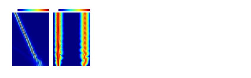
www.nature.com/scientificreports/
distinct domains of anomalous dispersion, separated by an interjacent domain of normal dispersion. A mutual
cross-phase modulation induced attractive potential provides the binding mechanism that holds the constituent
pulses together29. This transfers the concept of a soliton induced strong refractive index barrier for a normally
dispersive wave30, to the interaction of pulses in distinct domains of anomalous dispersion. The former process
is enabled by a general wave reflection mechanism originally reported in fluid dynamics31, in optics referred to
as the push-broom e ffect32, optical event h orizon33,34, or temporal r eflection35, allowing for a strong and efficient
36,37
all optical control of light p
ulses . This mechanism has been shown to naturally appear in the supercontinuum
generation process38–41. The previously studied formation of molecule-like two-frequency pulse compounds con-
stitutes a paradigmatic example of extreme states of light, also offering intriguing insights to atom-like features of
a soliton, including its ability to act as a localized trapping potential with a discrete level s pectrum29. For a higher-
order nonlinear Schrödinger equation with positive 2OD and negative 4OD, similar compound states where
recently also observed, and, along with the sech2–shaped single soliton solutions of earlier s tudies9,12, identified
as members of a large family of generalized dispersion Kerr s olitons42. Objects of this type have recently been
observed within a mode-locked laser c avity43. Dual-frequency pulses with similar pulse structure have previ-
ously also been studied experimentally in passively mode-locked fiber lasers44, and in a model for dual-channel
simultaneous modelocking based on the Swift-Hohenberg e quation45. Further, two-color soliton microcomb
states where reported in theoretical studies of Kerr microresonators in terms of the Lugiato-Lefever equation
(LLE) with two separate domains of anomalous dispersion46, and in the standard LLE with added negative quartic
group-velocity dispersion47. Bound states of distinct solitons, i.e. composite solitons, with a very similar pulse
structure where reported in a combined theoretical and experimental study of the Kerr multistability in the
LLE48. The properties of these kind of objects, which are referred to by a variety of names such as dual-frequency
pulses44, two-color soliton states46, two-frequency soliton molecules29, composite solitons48, and, polychromatic
soliton molecules43, are largely unexplored. Subsequently we refer to these objects simply as pulse compounds.
Here, we study the interaction dynamics of two initially superimposed fundamental solitons at distinctly
different center frequencies in terms of a propagation constant for which the group velocity dispersion (GVD)
has downward parabolic symmetry. Such a profile allows to parametrically define pairs of center frequencies at
which the local dispersion parameters have the same absolute values at any order. This reduces the complexity
of the underlying model and allows to explore the influence of the nonlinear interaction on the model dynamics
more directly. Specifically, we here investigate how an initial group-velocity (GV) mismatch affects the formation
of two-frequency pulse compounds. While it was shown that such compound states can compensate sufficiently
small GV mismatches through excitation of internal degrees of f reedom29, reminiscent of molecular vibrations,
this puts their robustness to the test and sheds more light on the binding mechanism that holds the subpulses
together. In the limit of large GV mismatch we observe a crossover from the formation of two-frequency com-
pound states to escaping solitons. We demonstrate that the crossover region exhibits pulse compounds consisting
of a strong trapping pulse and a weak trapped pulse, GV matched despite a large center frequency mismatch.
Building upon the interaction of a single soliton with a localized attractive potential in terms of a perturbed
NSE, we derive a simplified theoretical approach that suggests an analogy to classical mechanics and allows to
accurately estimate the parameter range wherein pulse compounds are formed.
Results
We model z-propagation of the real-valued optical field E(z, t) = ω Eω (z)e
−iωt in a periodic t-domain of extend
T with ω ∈ T Z in terms of the complex-valued analytic signal E (z, t) = 2 ω>0 Eω (z)e−iωt via the first-order
2π
nonlinear propagation equation
i∂z Eω + β(ω)Eω + γ (ω) |E |2 E ω>0 = 0, (1)
describing single mode propagation in a nonlinear waveguide49,50. In Eq. (1), β(ω) denotes the propagation
constant and γ (ω) specifies a coefficient function for its nonlinear part. The characteristics of both are illus-
trated in Fig. 1. Considering the reference frequency ω0 = 2 rad/fs, the propagation constant is modeled by the
polynomial expression
4
βn
β(ω) = (ω − ω0 )n , (2)
n!
n=0
with β0 = 25.0 µm−1, β1 = 13.0 fs µm−1, β2 = 0.1 fs2 µm−1, β3 = 0.0 fs3 µm−1, and β4 = −0.7 fs4 µm−1. For
our subsequent numerical analysis we consider the transformed field Eω′ (z) = Eω (z) exp(i vω0 z), shifted to a mov-
ing frame of reference. The time-domain representation E ′ (z, t) then corresponds to the time-shifted analytic
signal E (z, τ = t − z/v0 ). The reference velocity v0 is chosen so that the time-domain dynamics appears slow.
We subsequently set v0 ≡ vg (ω0 ) ≈ 0.0769 µm/fs , wherein vg (ω) ≡ [∂ω β(ω)]−1 signifies the group-velocity,
see Fig. 1a. As can be seen in Fig. 1b, the group velocity dispersion (GVD) β2 (ω) = ∂ω2 β(ω) assumes a down-
ward parabolic shape, which, in terms of the angular frequency detuning � = ω − ω0 , can be expressed as
β2 (ω0 + �) = β2 + β24 �2 . It is thus similar to the setup considered in reference42 in which a NSE subject to
positive quadratic and additional negative quartic dispersion was studied (see “Methods” for details). It is further
a simplified variant of the propagation constant with a non-symmetric GVD, for which we previously studied the
interaction of solitons leading to the formation of heteronuclear soliton
√ olecules29. Here, the zero-dispersion
m
detunings are given by the roots of the GVD at �ZDW1,ZDW2 = ± −2β2 /β4 ≈ ±0.535 rad/fs, specifying two
zero-dispersion frequencies at (ωZDW1 , ωZDW2 ) ≈ (1.465, 2.535) rad/fs. The coefficient function of the nonlin-
earity is modeled as
Scientific Reports | (2021) 11:11190 | https://doi.org/10.1038/s41598-021-90705-6 2
Vol:.(1234567890)www.nature.com/scientificreports/
a
b
c
Figure 1. Specifics of the considered z-propagation model. (a) Frequency dependence of the group velocity.
Frequency ranges shaded in red allow for group-velocity matched co-propagation of light pulses in separate
regions of anomalous dispersion. Horizontal dashed line indicates reference velocity v0. (b) Group velocity
dispersion profile. (c) Nonlinear coefficient function. In all subplots, normally dispersive frequency ranges are
shaded gray. Open circle and open square indicate the loci of ωGVM1 and ωGVM2, respectively. Thicker dashed
parts of curves indicate the angular frequency ranges covered by the parameter sweep. Polynomial models for
β(ω) and γ (ω) are detailed in the main text.
γ (ω) = γ0 + γ1 ω, (3)
with γ0 = 0.026 W−1 µm−1 and γ1 =0.321 fs W−1 µm−1, see Fig. 1c. To better understand the time-frequency
interrelations of the analytic signal at a selected propagation distance z, we consider its s pectrogram51
−iωτ ′ 2
1
(4)
′
′
PS (τ , ω) = E z, τ h τ − τ e dτ ,
2π
wherein h(x) = exp(−x 2 /2σ 2 ) specifies a Gaussian window function with root-mean-square width σ , used to
localize E (z, τ ) in time.
Equation (1) is free from the slowly varying envelope approximation but can be reduced to the generalized
nonlinear Schrödinger equation by introduction of a complex envelope for a suitable center f requency49. By
assuming γ = const., it can further be reduced to a standard NSE with higher orders of dispersion. For the
propagation of an initial field in terms of Eq. (1) we use a pseudospectral scheme implementing z-propagation
using a fourth-order Runge-Kutta m ethod52.
Initial conditions. As pointed out above, the GVD is symmetric about ω0 = 2 rad/fs. Two frequen-
cies are group-velocity√(GV) matched to ω0. In terms of the angular frequency detuning they are located
at �GVM1,GVM2 = ± −6β2 /β4 ≈ ±0.926 rad/fs, specifying group-velocity matched frequencies at
(ωGVM1 , ωGVM2 ) ≈ (1.074, 2.926) rad/fs, see Fig. 1a. Both frequencies are located in distinct domains of anoma-
lous dispersion realized by the considered propagation constant, see Fig. 1b. In general, group-velocity matched
co-propagation of anomalously dispersive light pulses is possible in the frequency ranges highlighted in red in
Fig. 1a. More specifically, for the considered propagation constant, a mode in range ω ∈ (0.931 rad/fs, ωZDW1 )
is GV matched to a mode in ω ∈ (ωZDW2 , 3.069 rad/fs).
Subsequently we will consider two fundamental solitons with duration t0 = 20 fs at distinctly dif-
ferent center frequencies ω1 = ωGVM1 − �ω and ω2 = ωGVM2 + �ω , with frequency offset parameter
�ω ∈ (−0.2, 0.2) rad/fs. A parameter sweep over these values of �ω covers the frequency ranges highlighted
by the thickened dashed curves in Fig. 1. A full initial condition for the real-valued optical field reads
E(0, t) = Re A1 e−iω1 t sech(t/t0 ) + A2 e−iω2 t sech(t/t0 ) . (5)
The initial pulses are specified by the amplitude condition for a fundamental soliton, given by
A1,2 = |β2 (ω1,2 )|/γ (ω1,2 )/t0 . Thus, for any considered value of �ω , both initial solitons will have match-
ing dispersion
√ lengths, i.e. LD,1 = LD,2 with LD,1 = t02 /|β2 (ω1 )| and LD,2 = t02 /|β2 (ω2 )|. However, since
A1 = γ (ω2 )/γ (ω1 )A2 , their amplitudes satisfy A1 > A2 . The group-velocity mismatch of both solitons
Scientific Reports | (2021) 11:11190 | https://doi.org/10.1038/s41598-021-90705-6 3
Vol.:(0123456789)www.nature.com/scientificreports/
vanishes only at �ω = 0 and increases for increasing absolute values of �ω . For example, for �ω < 0 one has
vg (ω1 ) ≥ v0 ≥ vg (ω2 ). In the considered frame of reference, a localized pulse with v < v0 will move towards
larger values of τ for increasing distance z.
The solitons injected at ω1 and ω2 are subject to higher orders of dispersion, which, in principle, causes
their velocities to slightly deviate from their bare group-velocities vg (ω1 ) and vg (ω2 ), respectively5,53. For a
soliton with center frequency ω s and duration ts , this might be taken into
account by considering a “corrected”
−1
soliton velocity54 vg′ (ωs , ts ) = β1 (ωs ) − β2 (ωs )/(ωs ts2 ) + β3 (ωs )/(6ts2 ) . For the full range of simulation
parameters considered in the presented study, the largest relative difference of these velocities was found to be
|vg − vg′ |/vg < 10−4 . Subsequently we opted to use the usual group-velocity vg when referring to the velocity of
the initial solitons.
Propagation dynamics of limiting cases. Our earlier study of the interaction dynamics of initially over-
lapping group-velocity matched fundamental solitons with a vast frequency gap29, suggests that in the limiting
case of group-velocity matched initial solitons [�ω = 0 rad/fs], a heteronuclear two-frequency pulse compound
will form. The evolution of a corresponding initial condition in the propagation range z = 0−25 mm is shown
in Fig. 2a. The composite pulse generated by this initial condition, highlighted in the spectrogram in Fig. 2b,
consists of two subpulses with roughly similar amplitudes but distinctly different center frequencies. From the
spectral intensity |Eω |2 and the spectrogram PS , the vast frequency gap between both subpulses is clearly evident.
It generates resonant radiation upon propagation and leads to a kind of “radiating” compound state. In Fig. 2b,
these resonances are signaled by trains of nodes that separate from the localized state. A thorough analysis of
a pulse compound with a similar composition was detailed in reference29 [see Fig. 2(f) of that reference]. The
binding mechanism that leads to the formation of such a composite pulse is realized by the mutual cross-phase
modulation between its interacting s ubpulses29. The resulting pulse compounds are quite robust: small initial
group-velocity mismatches can be compensated by frequency shifts of the subpulse center frequencies. This ena-
bles intriguing internal dynamics, reminiscent of molecular vibrations, examined more closely in Fig. 4 below.
In the limiting case of a large group-velocity mismatch of the initial solitons, i.e. for large absolute values of �ω ,
we expect that both pulses escape their mutual binding. This is demonstrated for �ω = −0.17 rad/fs in Fig. 2e,f.
As evident from the time-domain propagation dynamics in Fig. 2e, two separate localized states with nonzero
relative velocity can indeed be identified. They can be distinguished well in the spectrogram in Fig. 2f, indicating
no notable trapping by either pulse.
A crossover from the formation of two-frequency soliton compounds to escaping solitons can be expected
based on two arguments. First, consider the point of view of mutual trapping of each pulse by a cross-phase
modulation induced attractive potential formed by the other pulse29. Then, a classical mechanics interpretation
of the propagation scenario suggests the existence of an escape velocity, sufficient for a particle to escape its trap-
ping potential. We explore this analogy in more detail below. Second, for offset frequencies �ω > 0.143 rad/fs,
i.e. ω1 < 0.931 rad/fs and ω2 > 2.926 rad/fs, no mode can be group-velocity matched to either initial soliton, see
Fig. 1a. Having demonstrated the propagation dynamics for two specific values of the frequency offset param-
eter �ω , a thorough investigation of the crossover between the above limiting-cases in terms of �ω is in order.
Crossover from mutual trapping to escape. To better characterize the crossover from mutual trap-
ping to unhindered escape of the initial solitons, we track the velocities of the dominant localized pulses in
each domain of anomalous dispersion. In Fig. 3b, the asymptotic velocities associated with the initial solitons
at ω1 and ω2 are labeled v1 and v2, respectively. In relation to the two limiting cases illustrated earlier, we find
that at �ω = 0 rad/fs (cf. Fig. 2a) the velocities of the compounds subpulses match each other and are in good
agreement with the group-velocities of the initial solitons. At �ω = −0.17 rad/fs (cf. Fig. 2e) we find that the
dominant pulses in each region of anomalous dispersion are clearly distinct, again in agreement with the group-
(−)
velocities of the initial solitons. In between, a sudden crossover occurs at �ωc ≈ −0.075 rad/fs, where v2 shifts
(−) (−)
from v2 = v1 vg (ω1 ) [for �ωc < �ω < 0] to v2 = vg (ω2 ) [for �ω < �ωc ], see Fig. 3b.
(−)
Matching subpulse velocities in the range �ωc < �ω < 0 result from an initial transient propagation
regime during which the mutual interaction of the initially superimposed pulses causes both pulse center fre-
quencies to shift, thereby also changing the pulse spectrum. In this parameter range we observe that the soliton
with higher amplitude, i.e. the soliton initially at ω1, assumes a dominant role. While the effect on this pulse
is small, the effect on the pulse initially at ω2 is rather large. This is shown in Fig. 4, where we detail a simula-
tion run at �ω = −0.05 rad/fs. An initial transient behavior in range z < 10 mm is well visible, see Fig. 4a,b.
In the latter, the initial velocity mismatch of both pulses induces a vivid dynamics. This is demonstrated in
Fig. 4e, where the internal dynamics of the composite pulse in terms of the separation and relative-velocity of
its subpulses, reminiscent of molecular vibrations, is shown. For this example we find the asymptotic frequency
shifts ω1 = 1.124 rad/fs → ω1′ ≈ 1.113 rad/fs (Fig. 4c) and ω2 = 2.876 rad/fs → ω2′ ≈ 2.949 rad/fs (Fig. 4d).
The frequency up-shift ω2 → ω2′ is expected to result in a pulse velocity for which vg (ω2′ ) > vg (ω2 ) (cf. Fig. 1a).
More precisely, we find the velocity shift vg (ω2 ) = 0.076868 µm/fs → vg (ω2′ ) = 0.07695 µm/fs in agreement
with the data shown in Fig. 3b. As evident from Fig. 4a, radiation is emitted predominantly in the initial stage
of the pulse compounds formation process.
(−)
We find that in the vicinity of �ωc , the asymptotic state is characterized by two distinct pulse compounds.
The z-evolution of a corresponding initial condition at �ω = −0.1 rad/fs is shown in Fig. 2c,d. Therein, the time-
domain propagation dynamics (left panel of Fig. 2c) shows two localized pulses that separate from each other
for increasing propagation distance. As evident from the spectrogram at z = 25 mm (Fig. 2d), the two localized
pulses are actually pulse compounds (labeled C1 and C2 in Fig. 2d), each consisting of a strong trapping pulse
and a weak trapped pulse. An analogous phenomenon, referred to as development of a “soliton shadow”, “mixing”,
Scientific Reports | (2021) 11:11190 | https://doi.org/10.1038/s41598-021-90705-6 4
Vol:.(1234567890)www.nature.com/scientificreports/
a b
M
RR1
RR2
c d
C1 C2
e f
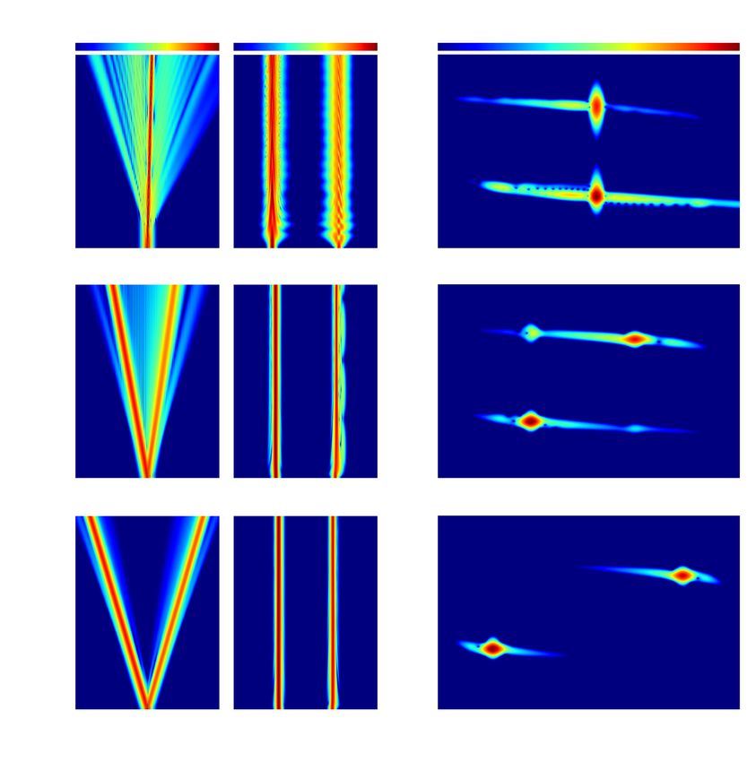
Figure 2. Exemplary propagation dynamics. (a) Evolution of the normalized time-domain intensity
|E (z, t)|2 /max[|E (z = 0 mm, t)|2 ] and normalized spectral intensity |Eω (z)|2 /max[|Eω (z = 0 mm)|2 ] of the
analytic signal for �ω = 0 rad/fs. Vertical dashed lines indicate zero dispersion points. (b) Analytic signal
spectrogram at z = 25 mm for �ω = 0 rad/fs. Horizontal dashed lines indicate zero dispersion points. Dashed
box (labeled M) encloses a molecule-like compound state. Trains of nodes signaling generation of resonant
radiation are labeled RR1 and RR2. (c,d) Same as (a,b) for �ω = −0.1 rad/fs. In (d), the two dashed boxes
(labeled C1 and C2) enclose pulse compounds each characterized by a strong trapping pulse and a weak trapped
pulse. (e,f) same as (a,b) for �ω = −0.18 rad/fs. Spectrograms are computed using σ = 20 fs in Eq. (4).
or “soliton-radiation trapping”, exists for coupled NSEs describing soliton propagation in birefringent fi bers21,25,
55
and gas-filled hollow-core photonic crystal fi bers . One of the main differences to other works is that we here
allow for group velocity matching across a vast frequency gap, which plays an important role in observing this
effect. For this reason, other studies of initially superimposed solitons with center frequency mismatch did not
observe such an effect56,57. Figure 5 shows a more comprehensive analysis of the individual pulse compounds. As
evident from Fig. 5a, the time-domain intensity of both pulse compounds exhibit a fringe pattern signaling the
superposition of subpulses with a significant center frequency mismatch. In Fig. 5b,c (Fig. 5d,e), the spectrum of
the compound labeled C1 [C2] is put under scrutiny. In either case, both subpulses are group velocity matched
and a phase-matching analysis for the strong trapping pulse indicates no generation of resonant radiation6,7, see
Fig. 5b,d. This is different from the radiating molecule in Fig. 2a.
(−)
For �ω < �ωc , i.e. beyond the crossover region, the trapping phenomenon changes qualitatively. This can
be seen from the overlap parameter
Scientific Reports | (2021) 11:11190 | https://doi.org/10.1038/s41598-021-90705-6 5
Vol.:(0123456789)www.nature.com/scientificreports/
a d
b e
c f
Figure 3. Characterization of the crossover from mutual trapping to escape. (a–c) Results for γ (ω) given by
Eq. (3). (a) Point particle motion in an attractive potential. The particle can escape the well if its kinetic energy
class exceeds the potential depth U (see text for details). Parameter range in which the particle cannot escape
Tkin 0
the well is shaded gray. Secondary ordinate shows the trapping coefficient Ctr computed in a simplified model
for a soliton interacting with a localized attractive potential (see text for details). (b) Comparison of observed
asymptotic velocities v1 and v2 of the dominant localized pulses in the distinct domains of anomalous dispersion
and corresponding propagation constant based group-velocities vg . Light-green solid and dashed lines indicate
the group velocities vg (ω1′ ) and vg (ω2′ ), obtained for the shifted pulse center frequencies ω1′ and ω2′ , respectively
(see text for details). (c) Logarithm of the overlap parameter q at z = 25 mm, quantifying the degree of mutual
trapping (see text for details). Shaded area beyond �ω ≈ 0.143 rad/fs indicates region in which group-velocity
matching cannot be achieved, cf. Fig. 1a. (d–f) Same as (a–c) considering γ (ω) = γ0.
c e
d
Figure 4. Formation of a two-frequency pulse compound at �ω = −0.05 rad/fs. Evolution of (a) normalized
time-domain intensity |E (z, t)|2 /max[|E (z = 0 mm, t)|2 ] (shown on linear scale), and (b) normalized spectrum
|Eω (z)|2 /max[|Eω (z = 0 mm)|2 ]. (c) Spectrum in the frequency range (0.8, 1.5) rad/fs, showing the initial
spectrum at z = 0 mm (labeled A), the full spectrum at z = 25 mm (labeled B), and a filtered spectrum at
z = 25 mm (labeled C), which excludes the free radiation and highlights the subpulse in the shown frequency
range. Superimposed arrow indicates direction and size of observed frequency shift (numeric values are quoted
in the text). (d) Same as (c) for frequency range (2.5, 3.3) rad/fs. In (c,d) the domain of normal dispersion is
shaded gray. (e) Internal dynamics of the pulse compound described in terms of separation ( tp) and relative
velocity ( vp) of its subpulses. Trajectory in (�tp , �vp )-plane is shown for z > 4 mm. Markers indicate
propagation distances (z1 , z2 , z3 ) = (4, 5, 6) mm.
Scientific Reports | (2021) 11:11190 | https://doi.org/10.1038/s41598-021-90705-6 6
Vol:.(1234567890)www.nature.com/scientificreports/
a
C1
C2
b d
c e
Figure 5. Detailed analysis of the pulse compounds C1 and C2 of Fig. 2d at z = 25 mm. (a) Normalized time-
domain intensity |E |2 /max[|E |2 ]. (b) Phase matching analysis for the strong trapping pulse of C1. Shift of the
soliton wavenumber qC1 = γ (ωC1 ′ )P /2 and wavenumber D (ω) = β(ω) − β(ω′ ) − β (ω′ )(ω − ω′ ),
0 C1 C1 1 C1 C1
where P0 is the peak intensity of the strong trapping pulse and ωC1′ is its center frequency. Local extrema indicate
group velocity matching with the strong trapping pulse. Frequencies at which resonant radiation might be
expected are indicated by the roots of qC1 − DC1 (ω). (c) Normalized spectrum |Eω (z)|2 /max[|Eω (z = 0 mm)|2 ]
showing the initial spectrum at z = 0 mm (labeled A), full spectrum at z = 25 mm (labeled B), and spectra of
the strong trapping pulse (labeled C) and weak trapped pulse (labeled D) of C1. (d,e) Same as (b,c) for C2.
I1 (z)I2 (z) dτ
q(z) = , (6)
I1 (0)I2 (0) dτ
in which I1 (z) = | ωωZDW2 Eω (z)e−iωt |2 are the time-domain intensity
profiles of the pulse components restricted to separate regions of anomalous dispersion. It quantifies the degree
of mutual trapping and is shown in Fig. 3c. For the limiting case of the soliton molecule (�ω = 0 rad/fs; Fig. 2a)
(−)
we find q ≈ 2.1 at z = 25 mm. In the range �ω < �ωc , i.e. progressing towards increasingly negative values of
the frequency offset parameter, it shows an exponential decrease in support of a strong-trapping to weak-trapping
transition. We find this also confirmed by comparing the spectrograms in Fig. 2d,f.
A similar crossover occurs for increasing positive values of the frequency offset parameter at
(+) (+)
�ωc ≈ 0.08 rad/fs . For �ω < �ωc the values of v2 and v1 coincide and are again in well agreement with
(+)
vg (ω1 ), see Fig. 3b. For �ω < �ωc , v2 crosses over to a value that follows the trend of vg (ω2 ), but exhibits
the systematic deviation vg (ω2 ) − v2 ≈ 0.00007 µm/fs. This systematic deviation is again a consequence of the
perturbation imposed by the presence of a superimposed pulse in the initial condition. As pointed out earlier, the
direct overlap of two solitons at z = 0 mm leads to an initial transient stage, during which their mutual interac-
tion causes both pulse center frequencies to shift. Here, the effect on the pulse initially at ω1 is again small and
the effect on the pulse initially at ω2 is rather large. Analyzing the simulation run at �ω = 0.12 rad/fs, we find
the frequency shifts ω1 = 0.954 rad/fs → ω1′ ≈ 0.961 rad/fs and ω2 = 3.046 rad/fs → ω2′ ≈ 2.991 rad/fs. The
frequency down-shift ω2 → ω2′ is expected to result in a pulse velocity for which vg (ω2′ ) < vg (ω2 ) (cf. Fig. 1a).
As evident from Fig. 3b, the pulse velocities vg (ω1′ ) and vg (ω2′ ) obtained for the shifted center frequencies are
in excellent agreement with the observed pulse velocities (see light-green solid and dashed lines in Fig. 3b).
As pointed out above, beyond �ω = 0.143 rad/fs , group velocity matching is not possible (shaded region in
Fig. 3). This is reflected by the overlap parameter q, dropping down to negligible values for �ω > 0.143 rad/fs.
We observe a shift of both pulse center frequencies towards each other for �ω > 0, while they shift away from
each other for �ω < 0 (see the example detailed in Figs. 4c,d). This results in group-velocity matching in the
domain where pulse compounds are formed, This is different from studies of the unperturbed NSE, where the
center frequencies of initially overlapping solitons where reported to shift towards each other for any reasonable
initial frequency s eparation58.
To clarify how the term ∝ γ1 ω in the definition of γ (ω) [Eq. (3)] affects our observations, we repeated the
above parameter study using the modified coefficient function γ (ω) = γ0. This setting can be reduced to a stand-
ard NSE with higher orders of dispersion (see “Methods” for details), similar to the model in which generalized
dispersion Kerr solitons were studied r ecently42. Considering this simplified coefficient function, the above
Scientific Reports | (2021) 11:11190 | https://doi.org/10.1038/s41598-021-90705-6 7
Vol.:(0123456789)www.nature.com/scientificreports/
parameter study involves two initial solitons with matching dispersion lengths [LD,1 = LD,2] and equal amplitudes
[ A1 = A2]. As shown in Fig. 3e, across the region of compound state formation (i.e. for |�ω| < 0.065 rad/fs), the
asymptotic velocities v1 and v2 are not longer dominated by any particular pulse. Instead, the resulting composite
pulse has velocity v0. This is, again, achieved by a shift of the pulses center frequencies during an initial tran-
sient stage. In comparison to the case where γ (ω) is modeled via Eq. (3), we find that the region of compound
state formation is narrower. Despite the higher orders of dispersion featured by Eq. (1), the results reported in
Fig. 3e are in good qualitative agreement with the interaction dynamics of initially overlapping, group-velocity
mismatched solitons in a model of two nonlinearly coupled N SEs56. Also, a systematically smaller value of the
overlap parameter q is evident in Fig. 3f. Let us comment on the characteristics of the pulse compounds in the
vicinity of the crossover. The distinct features of C1 and C2 in Fig. 5 are solely due to the unsymmetry caused
by the coefficient function γ (ω) given by Eq. (3). Considering the above modified coefficient function, we find
that the spectra of C1 and C2 are simply related by symmetry, i.e. we can obtain C2 by inversion of C1 about
ω0 = 2 rad/fs.
Discussion
For the whole range of frequency offsets considered in our numerical simulations, we find that the observed
velocity v1 closely follows the group velocity vg (ω1 ). Both are associated with the initial fundamen-
tal soliton with the larger amplitude. We here find that the observed velocity v2 can match v1 in the range
−0.075 rad/fs < �ω < 0.08 rad/fs , specifying the range within which heteronuclear pulse compounds are
formed by the considered initial conditions. Outside this range, the formation of a single two-frequency soliton
molecule is inhibited, with two localized pulses separating from each other and suppressed trapping for large
absolute values of the frequency offset parameter.
We found that we can estimate the domain of molecule formation in terms of a simplified theoretical approach
(see “Methods” for details). In the latter, the dynamics of a two-pulse initial condition of the form of Eq. (5), gov-
erned by the nonlinear propagation equation Eq. (1), is approximated by the dynamics of a single pulse evolving
under a nonlinear Schrödinger equation with localized attractive potential, given by
β2′ 2
′
′ ′
′
′
′
2 ′
i∂z φ z, τ + iβ1 ∂τ − ∂τ ′ − U τ + γ |φ z, τ | φ z, τ = 0. (7)
2
Therein the complex envelope φ(z, τ ′ ) describes the dynamics of the subpulse with smaller amplitude, i.e.
the subpulse at ω2. The potential well U(τ ′ ) is related to the subpulse with higher amplitude, i.e. the subpulse at
ω1, and is given by U(τ ′ ) = −U0 sech2 (τ ′ /t0 ) with potential depth
γ (ω2 ) |β2 (ω1 )|
U0 = 2 . (8)
γ (ω1 ) t02
Further, β1′ = β1 (ω2 ) − β1 (ω1 ), β2′ = β2 (ω2 ), γ ′ = γ (ω2 ), and τ ′ = t − β1 (ω1 )z . A similar approxima-
tion, for the special case of group-velocity matched propagation β1′ = 0 , was recently used to demonstrate
trapped states in a soliton-induced refractive index w ell29. Equation (7) suggests an analogy to a one-dimensional
Schrödinger equation for a fictitious particle of mass m = −1/β2′ , evolving in an attractive potential localized
along the τ ′ axis. The relative velocity between the soliton and the potential is β1′ . From a classical mechanics point
of view we might expect that a particle, initially located at the potential center at τ ′ = 0, escapes the potential
well if its “classical” kinetic energy along the τ ′-axis, given by
m ′2 [β1 (ω2 ) − β1 (ω1 )]2
class
Tkin = β1 = − , (9)
2 2β2 (ω2 )
exceeds the potential depth U0. In other words, for Tkin class < U we expect the particle to remain trapped by the
0
potential. For the original model, defined by Eq. (1), this might be used to approximately estimate the domain in
which compound states are formed. The results of this simplified theoretical approach are summarized in Fig. 3a,d,
where Tkin
class and U are shown as function of the frequency offset parameter �ω . For example, considering the
0
setup with γ (ω) defined by Eq. (3), the condition Tkinclass < U is satisfied for −0.068 rad/fs < �ω < 0.098 rad/fs
0
(Fig. 3a). Despite the various simplifying assumptions that led to the above trapping condition, the estimated
bounds for the domain of compound state formation are in excellent agreement with the observed bounds dis-
cussed above. In Fig. 3a,d we complement the findings based on the classical mechanics analogy by probing the
trapping-to-escape transition of a soliton in a potential well in terms of Eq. (20) via numerical simulations. We
therefore computed a trapping coefficient, defined by
1 10 t0
′
2 ′
Ctr = |φ z, τ | dτ , (10)
N −10 t0
with N = |φ(0, τ ′ )|2 dτ ′ for z = 10 mm. Both are in excellent qualitative agreement.
In conclusion, we showed that there exists a limit in the group-velocity mismatch of the constituents of
a solitonic two-frequency pulse compound, above which its existence is not possible anymore. We clarified
the breakup dynamics for the compound states beyond that limit, and showed that every constituent takes
away parts of the radiation, again depending on the relative group velocities. The velocity of the pulse com-
pound before the breakup is determined mostly by its “heaviest” component. More generally, our work demon-
strates clearly the limits of stability of multicolor solitonic pulse compounds and we expect that the presented
Scientific Reports | (2021) 11:11190 | https://doi.org/10.1038/s41598-021-90705-6 8
Vol:.(1234567890)www.nature.com/scientificreports/
crossover-phenomenon will be useful for studying and understanding the break-up dynamics of more complex
olecules43.
multi-frequency compounds, such as the recently demonstrated polychromatic soliton m
Methods
Below we derive a simplified theoretical model, allowing to estimate the parameter range of �ω that supports
formation of two-frequency pulse compounds discussed in the main text. Starting point of our consideration is
the first order nonlinear propagation equation for the analytic signal [Eq. (1)], with propagation constant β(ω)
and coefficient function γ (ω) given by Eqs. (2) and (3), respectively, together with initial conditions of the form
of Eq. (5). We then make the following assumptions and approximation steps:
1. Introducing a reference frequency and shifting to a moving frame of r eference49. We choose the reference
frequency ω0, for which β(ω0 ) = β0 and β1 (ω0 ) = β1, and consider the frequency detuning � = ω − ω0 to
define the complex envelope
ψ(z, τ ) = ψ� (z)e−i�τ , with ψ� (z) = Eω0 +� (z)e−i(β0 +β1 �)z , and τ = t − β1 z, (11)
�
for which Eq. (1) takes the form
i∂z ψ� + [β(ω0 + �) − β0 − β1 �]ψ� + γ (ω0 + �) |ψ|2 ψ � = 0. (12)
The initial condition Eq. (5) then reads
ψ(0, τ ) = A1 e−i�1 τ + A2 e−i�2 τ sech(τ/t0 ), (13)
with �1,2 = ω1,2 − ω0 and A1,2 = |β2 (ω0 + �1,2 )|/γ (ω0 + �1,2 )/t0 . Let us note that, considering
β(ω0 + �) given by Eq. (2), and γ (ω0 + �) = γ0, allows to simplify Eq. (12) to the higher-order nonlinear
Schrödinger equation
β2 2 β4 4
� + � ψ� + γ0 |ψ|2 ψ � = 0. (14)
i∂z ψ� +
2 24
For parameter values β2 > 0 and β4 < 0, as we do consider here [see parameters listed right after Eq. (2)],
Eq. (14) specifies the frequency domain representation of the model in which generalized dispersion Kerr
solitons where d emonstrated42.
2. Approximating the dynamics of a two-pulse initial condition [Eq. (13)], governed by Eq. (12), by a system
of coupled higher-order nonlinear Schrödinger equations. Therefore, we define two distinct fields
χ (1,2) (z, τ ) = (1,2)
χ̟ (z)e−i̟ τ , (15)
̟
taken at the center frequencies 1,2 of the two pulses with ̟ denoting the respective frequency detuning,
and consider instead of Eq. (12) the pair of coupled equations
(1) (1) β2(1) 2 β3(1) 3 β4(1) 4
(1)
i∂z χ̟ + β0 + β1 ̟ + ̟ + ̟ + ̟ χ̟ (1)
+ γ (1) |χ (1) |2 χ (1) + 2|χ (2) |2 χ (1) = 0, (16)
2 6 24 ̟
(2) (2) β2(2) 2 β3(2) 3 β4(2) 4
(2)
i∂z χ̟ + β0 + β1 ̟ + ̟ + ̟ + ̟ χ̟ (2)
+ γ (2) |χ (2) |2 χ (2) + 2|χ (1) |2 χ (2) = 0. (17)
2 6 24 ̟
In the linear parts of Eqs. (16, 17) we introduced the modified dispersion parameters
(1,2)
βn ≡ ∂� n
[β(ω0 + �) − β0 − β1 �]�=�1,2, local to the center frequencies of both pulses. In the nonlinear
parts of Eqs. (16, 17) we made the simplifying assumptions γ (1,2) = γ (ω0 + �1,2 ) and kept only the effects of
self-phase modulation and mutual cross-phase modulation. We might then approximate the dynamics of an
initial condition of the form of Eq. (13), evolving under the single equation Eq. (12), by the pair of coupled
equations Eqs. (16, 17) with initial conditions
χ (1,2) (0, τ ) = A1,2 sech(τ/t0 ), where A1,2 = |β2(1,2) |/γ (1,2) /t0 . (18)
Thereby we further assume the spectral width of either pulse to be small compared to the separa-
tion of the pulses center frequencies. Let us note that in the special case where we use Eq. (12) to sim-
ulate the dynamics of a single pulse initial condition ψ(0, τ ) = A1 e−i�1 τ sech(τ/t0 ) we can write
χ (z, τ ) = ̟ ψ�1 +̟ e−i̟ τ = ψ(z, τ )ei�1 τ , so that χ(0, τ ) = A1 sech(τ/t0 ) follows immediately.
(1)
(1,2)
3. We make the simplifying assumption that βn = 0 for n > 2 in Eqs. (16, 17) and neglect the cross-
phase modulation contribution in Eq. (16). The latter implies that the dynamics of χ (1), which rep-
resents the pulse with larger amplitude, is not affected by χ (2). Under these assumptions, Eq. (16) with
χ (1) (0, τ ) = A1 sech(τ/t0 ) constitutes a standard nonlinear Schrödinger equation for a fundamental soliton.
We may further use the transformation
Scientific Reports | (2021) 11:11190 | https://doi.org/10.1038/s41598-021-90705-6 9
Vol.:(0123456789)www.nature.com/scientificreports/
(2) (1)
′ −i β0 +β1 ̟ z (1)
φ(z, τ ′ ) = φ̟ e−i̟ τ , (2)
with φ̟ (z) = χ̟ (z)e , and τ ′ = τ − β1 z, (19)
̟
(2)
to formally remove the term ∝ β0 from Eq. (17) and shift to a reference frame in
which |χ (2) |2 is stationary. Abbreviating �β1 ≡ β1(2) − β1 and introducing the potential
(1)
U(τ ′ ) ≡ −2γ (2) |χ (1) (0, τ ′ )|2 = −2γ (2) A21 sech2 (τ ′ /t0 ) we obtain
β2(2) 2
i∂z φ̟ + �β1 ̟ + ̟ φ̟ + γ (2) |φ|2 φ − Uφ = 0. (20)
2 ̟
We further consider the single soliton initial condition φ(0, τ ′ ) = A2 sech(τ ′ /t0 ) [cf. Eq. (18)], initially
l o c a l i z e d at t h e c e nte r
of t h e p ote nt i a l we l l. L e t u s n ote t h at i n E q. ( 1 9 )
τ ′ = t − β1 + β2 �1 + β64 �31 z = t − β1 (ω0 + �1 )z , which verifies that Eq. (20) is in a reference frame
in which the potential, representing the pulse at ω1 = ω0 + �1, is at rest.
The time-domain representation of Eq. (20), given by
′ β2(2) 2 2
i∂z φ(z, τ ) + i�β1 ∂τ ′ − ∂ ′ − U(τ ) + γ |φ(z, τ )| φ(z, τ ′ ) = 0,
′ (2) ′
(21)
2 τ
constitutes the simplified model which allows to estimate the parameter range in which two-frequency pulse
compounds are formed (see Discussion in the main text). Let us note that Eq. (21) represents a nonlinear
Schrödinger equation with an attractive external potential of sech-squared shape. Similar model equations were
previously used to study soliton-defect collisions in the nonlinear Schrödinger equation59,60, and interaction
of matter-wave solitons with quantum wells in the one-dimensional Gross-Pitaevskii e quation61. While these
studies considered the collision of a soliton with an external attractive potential, our aim is here to understand
the escape of a soliton from such a potential.
Received: 26 February 2021; Accepted: 13 May 2021
References
1. Drazin, P. G. & Johnson, R. S. Solitons: An Introduction (Cambridge University Press, 1989).
2. Kivshar, Y. S. & Agrawal, G. P. Optical Solitons: From Fibers to Photonic Crystals (Academic Press, 2003).
3. Mitschke, F. Fiber Optics: Physics and Technology (Springer, 2010).
4. Stegeman, G. I. & Segev, M. Optical spatial solitons and their interactions: Universality and diversity. Science 286, 1518–1523
(1999).
5. Akhmediev, N. & Karlsson, M. Cherenkov radiation emitted by solitons in optical fibers. Phys. Rev. A 51, 2602 (1995).
6. Yulin, A. V., Skryabin, D. V. & Russel, P. S. J. Four-wave mixing of linear waves and solitons in fibers with higher-order dispersion.
Opt. Lett. 29, 2411 (2004).
7. Tsoy, E. N. & de Sterke, C. M. Theoretical analysis of the self-frequency shift near zero-dispersion points: Soliton spectral tunneling.
Phys. Rev. A 76, 043804 (2007).
8. Höök, A. & Karlsson, M. Ultrashort solitons at the minimum-dispersion wavelength: Effects of fourth-order dispersion. Opt.
Commun. 18, 1388 (1993).
9. Karlsson, M. & Höök, A. Soliton-like pulses governed by fourth-order dispersion in optical fibers. Opt. Commun. 104, 303 (1994).
10. Piché, M., Cormier, J. F. & Zhu, X. Bright optical soliton in the presence of fourth-order dispersion. Opt. Lett. 21, 845 (1996).
11. Blanco-Redondo, A. et al. Pure-quartic solitons. Nat. Commun. 7, 10427 (2016).
12. Kruglov, V. I. & Harvey, J. D. Solitary waves in optical fibers governed by higher-order dispersion. Phys. Rev. A 98, 063811 (2018).
13. Schürmann, H. W. & Serov, V. Comment on “Solitary waves in optical fibers governed by higher-order dispersion”. Phys. Rev. A
100, 057801 (2019).
14. Kruglov, V. I. & Harvey, J. D. Reply to “Comment on “Solitary waves in optical fibers governed by higher-order dispersion””. Phys.
Rev. A 100, 057802 (2019).
15. Kruglov, V. I. Solitary wave and periodic solutions of nonlinear Schrödinger equation including higher order dispersions. Opt.
Commun. 472, 125866 (2020).
16. Kruglov, V. I. & Triki, H. Quartic and dipole solitons in a highly dispersive optical waveguide with self-steepening nonlinearity
and varying parameters. Phys. Rev. A 102, 043509 (2020).
17. Stratmann, M., Pagel, T. & Mitschke, F. Experimental observation of temporal soliton molecules. Phys. Rev. Lett. 95, 143902 (2005).
18. Ueda, T. & Kath, W. L. Dynamics of coupled solitons in nonlinear optical fibers. Phys. Rev. A 42, 564 (1990).
19. Afanas’ev, V. V., Dianov, E. M., Prokhorov, A. M. & Serkin, V. N. Nonlinear pairing of light and dark optical solitons. Pisma Zh.
Eksp. Teor. Fiz. 48, 588 (1988) (JETP Lett. 48, 638 (1988)).
20. Trillo, S., Wabnitz, S., Wright, E. M. & Stegeman, G. I. Optical solitary waves induced by cross-phase modulation. Opt. Lett. 13,
871 (1988).
21. Menyuk, C. R. Stability of solitons in birefringent optical fibers. II. Arbitrary amplitudes. J. Opt. Soc. Am. B 5, 392 (1988).
22. Afanasjev, V. V., Dianov, E. M. & Serkin, V. N. Nonlinear pairing of short bright and dark soliton pulses by phase cross modulation.
IEEE J. Quantum Electron. 25, 2656 (1989).
23. Afanasyev, V. V., Kivshar, Yu. S., Konotop, V. V. & Serkin, V. N. Dynamics of coupled dark and bright optical solitons. Opt. Lett.
14, 805 (1989).
24. Menyuk, C. R. Pulse propagation in an elliptically birefingent Kerr medium. IEEE J. Quantum Electron. 25, 2674 (1989).
25. Cao, X. D. & Meyerhofer, D. D. Soliton collisions in optical birefringent fibers. J. Opt. Soc. Am. B 11, 380 (1994).
26. Oreshnikov, I., Driben, R. & Yulin, A. Dispersive radiation and regime switching of oscillating bound solitons in twin-core fibers
near zero-dispersion wavelength. Phys. Rev. A 96, 013809 (2017).
27. Krupa, K., Nithyanandan, K., Andral, U., Tchofo-Dinda, P. & Grelu, P. Real-time observation of internal motion within ultrafast
dissipative optical soliton molecules. Phys. Rev. Lett. 118, 243901 (2017).
Scientific Reports | (2021) 11:11190 | https://doi.org/10.1038/s41598-021-90705-6 10
Vol:.(1234567890)www.nature.com/scientificreports/
28. Wang, Z. Q., Nithyanandan, K., Coillet, A., Tchofo-Dinda, P. & Grelu, P. Optical soliton molecular complexes in a passively mode-
locked fibre laser. Nat. Commun. 10, 830 (2019).
29. Melchert, O. et al. Soliton molecules with two frequencies. Phys. Rev. Lett. 123, 243905 (2019).
30. Demircan, A., Amiranashvili, Sh. & Steinmeyer, G. Controlling light by light with an optical event horizon. Phys. Rev. Lett. 106,
163901 (2011).
31. Smith, R. The reflection of short gravity waves on a non-uniform current. Math. Proc. Cambridge Philos. Soc. 78, 517 (1975).
32. de Sterke, C. M. Optical push broom. Opt. Lett. 17, 914 (1992).
33. Philbin, T. G. et al. Fiber-optical analog of the event horizon. Science 319, 1367 (2008).
34. Faccio, D. Laser pulse analogues for gravity and analogue Hawking radiation. Cont. Phys. 1, 1 (2012).
35. Plansinis, B. W., Donaldson, W. R. & Agrawal, G. P. What is the temporal analog of reflection and refraction of optical beams?.
Phys. Rev. Lett. 115, 183901 (2015).
36. Demircan, A., Amiranashvili, Sh., Brée, C. & Steinmeyer, G. Compressible octave spanning supercontinuum generation by two-
pulse collisions. Phys. Rev. Lett. 110, 233901 (2013).
37. Demircan, A., Amiranashvili, Sh., Brée, C., Morgner, U. & Steinmeyer, G. Adjustable pulse compression scheme for generation of
few-cycle pulses in the midinfrared. Opt. Lett. 39, 2735 (2014).
38. Driben, R., Mitschke, F. & Zhavoronkov, N. Cascaded interactions between Raman induced solitons and dispersive waves in
photonic crystal fibers at the advanced stage of supercontinuum generation. Opt. Express 18, 25993 (2010).
39. Demircan, A. et al. Rogue events in the group velocity horizon. Sci. Rep. 2, 850 (2012).
40. Demircan, A. et al. Rogue wave formation by accelerated solitons at an optical event horizon. Appl. Phys. B 115, 343 (2014).
41. Armaroli, A., Conti, C. & Biancalana, F. Rogue solitons in optical fibers: A dynamical process in a complex energy landscape?.
Optica 2, 497 (2015).
42. Tam, K. K. K., Alexander, T. J., Blanco-Redondo, A. & de Sterke, C. M. Generalized dispersion Kerr solitons. Phys. Rev. A 101,
043822 (2020).
43. Lourdesamy, J. P., Runge, A. F. J., Alexander, T. J., Hudson, D. D., Blanco-Redondo, A. & de Sterke, C. M. Polychromatic soliton
molecules. Preprint at https://arxiv.org/abs/2007.01351 (2020).
44. Hu, G. et al. Asynchronous and synchronous dual-wavelength pulse generation in a passively mode-locked fiber laser with a
mode-locker. Opt. Lett. 42, 4942 (2017).
45. Zhang, X. et al. Design of a dual-channel modelocked fiber laser that avoids multi-pulsing. Opt. Exp. 27, 14173 (2019).
46. Moille, G., Li, Q., Kim, S., Westly, D. & Srinivasan, K. Phased-locked two-color single soliton microcombs in dispersion-engineered
Si3 N4 resonators. Opt. Lett. 43, 2772 (2018).
47. Melchert, O., Yulin, A. & Demircan, A. Dynamics of localized dissipative structures in a generalized Lugiato-Lefever model with
negative quartic group-velocity dispersion. Opt. Lett. 45, 2764 (2020).
48. Weng, W., Bouchand, R. & Kippenberg, T. J. Formation and collision of multistability-enabled composite dissipative Kerr solitons.
Phys. Rev. X 10, 021017 (2020).
49. Amiranashvili, Sh. & Demircan, A. Hamiltonian structure of propagation equations for ultrashort optical pulses. Phys. Rev. A 82,
013812 (2010).
50. Amiranashvili, Sh. & Demircan, A. Ultrashort optical pulse propagation in terms of analytic signal. Adv. Opt. Technol. 2011, 989515
(2011).
51. Melchert, O., Roth, B., Morgner, U. & Demircan, A. OptFROG—Analytic signal spectrograms with optimized time-frequency
resolution. SoftwareX 10, 100275 (2019).
52. Melchert, O., Morgner, U.Roth, B., Babushkin, I. & Demircan, A. Accurate propagation of ultrashort pulses in nonlinear waveguides
using propagation models for the analytic signal. In Computational Optics II (eds. Smith, D. G. et al.) 103–113 (SPIE, 2018).
53. Haus, H. A. & Ippen, E. P. Group velocity of solitons. Opt. Lett. 26, 1654 (2001).
54. Pickartz, S., Bandelow, U. & Amiranashvili, Sh. Adiabatic theory of solitons fed by dispersive waves. Phys. Rev. A 94, 033811 (2016).
55. Saleh, M. F. & Biancalana, F. Soliton-radiation trapping in gas-filled photonic crystal fibers. Phys. Rev. A 87, 043807 (2013).
56. Afanasjev, V. V. & Vysloukh, V. A. Interaction of initially overlapping solitons with different frequencies. J. Opt. Soc. Am. B 11,
2385 (1994).
57. Feigenbaum, E. & Orenstein, M. Coherent interactions of colored solitons via parametric processes: Modified perturbation analysis.
J. Opt. Soc. Am. B 22, 1414 (2005).
58. Kodama, J. & Hasegawa, A. Effects of initial overlap on the propagation dynamics of optical solitons at different wavelengths. Opt.
Lett. 16, 208 (1991).
59. Cao, X. D. & Malomed, B. A. Soliton-defect collisions in the nonlinear Schrödinger equation. Phys. Lett. A 206, 177 (1995).
60. Goodman, R. H., Holmes, P. J. & Weinstein, M. I. Strong NLS soliton-defect interactions. Phys. D 192, 215 (2004).
61. Ernst, T. & Brand, J. Resonant trapping in the transport of a matter-wave soliton through a quantum well. Phys. Rev. A 81, 033614
(2010).
Acknowledgements
The authors acknowledge financial support from the Deutsche Forschungsgemeinschaft (DFG) under Germany’s
Excellence Strategy within the Clusters of Excellence PhoenixD (Photonics, Optics, and Engineering – Innovation
Across Disciplines) (EXC 2122, projectID 390833453) and QuantumFrontiers (EXC 2123, projectId 390837967).
Author contributions
O.M. performed the numerical simulations and analysis. S.W. supported the numerical simulations. O.M.,
S.W., U.M., I.B. and A.D. interpreted the results and contributed to the manuscript. A.D. headed the project
throughout.
Funding
Open Access funding enabled and organized by Projekt DEAL.
Competing interests
The authors declare no competing interests.
Additional information
Correspondence and requests for materials should be addressed to O.M.
Reprints and permissions information is available at www.nature.com/reprints.
Scientific Reports | (2021) 11:11190 | https://doi.org/10.1038/s41598-021-90705-6 11
Vol.:(0123456789)You can also read