On articulated plates with micro-slits to tackle low-frequency noise
←
→
Page content transcription
If your browser does not render page correctly, please read the page content below
Acta Acustica 2021, 5, 31
Ó M.E. D’Elia et al., Published by EDP Sciences, 2021
https://doi.org/10.1051/aacus/2021024

                                                                                                                        Available online at:
                                                                                                         https://acta-acustica.edpsciences.org

 SCIENTIFIC ARTICLE

On articulated plates with micro-slits to tackle low-frequency noise
Massimo Emiliano D’Elia* , Thomas Humbert , and Yves Aurégan
Laboratoire d’Acoustique de l’Université du Mans, LAUM-UMR CNRS 6613, Avenue Olivier Messiaen, 72085 Le Mans Cedex 9,
France

            Received 13 April 2021, Accepted 21 June 2021

            Abstract – In recent years, new concepts of acoustic absorbers dedicated to the reduction of low-frequency
            noise have been developed. Among them, liners with moving parts, such as membrane-based liners, have been
            an object of particular interest. In the present paper, we propose a liner concept based on a cantilever beam
            made of articulated plates with micro-slits. Compared to membrane technologies, these micro-slits introduce
            a small leakage from the backing cavity that reduces the high compressibility effects occurring at very low fre-
            quencies in a small cavity. An acoustic liner including an ensemble of such articulated plates has been fabricated
            and characterized for grazing acoustic incidence in absence and in presence of flow. Measurements in an impe-
            dance tube at normal incidence have also been performed, and perfect absorption is obtained at a frequency
            where the liner thickness corresponds to 1/16th of the acoustic wavelength. A new and simple model is proposed
            to predict the attenuation of this type of acoustic treatment. The results are in good agreement with the mea-
            surements, indicating a correct identification of the physical phenomena here at stake.

            Keywords: Acoustic materials, Metamaterials, Vibrating beams

1 Introduction                                                              [1, 11]. Therefore, in the case of high sound levels or in
                                                                            the presence of flow, the additional constraint of having a
    Reducing low-frequency sound with small size devices                    high open area ratio is also required in the design of these
remains challenging. As a result, various new sound absor-                  new materials.
ber concepts for the reduction of low-frequency noise have                      In this regard, the use of elastic membranes and deco-
been developed in recent years. Conventional locally react-                 rated elastic membranes as sound absorbers is an interest-
ing absorbers consist of a honeycomb structure acting as a                  ing option [13–16]. In this case, the membrane can
cavity and a perforated or micro-perforated plate where the                 represent a large part of the total surface area and the fre-
air in the holes acts as a resistance and also as an oscillating            quency can easily be reduced by increasing the added mass
mass [1, 2]. In this case, the resonance frequency is some-                 [17]. The effect of a grazing flow has already been studied on
where between the quarter-wave resonance of the cavity                      this type of structure [18, 19], however it has the disadvan-
(f = c0/4B where c0 is the speed of sound and B is the                      tage of containing an encapsulated volume of air which can
height of the cavity)     and  ffi the Helmholtz resonance fre-
                     pffiffiffiffiffiffiffiffiffiffi                                            expand in the presence of a depression causing static defor-
quency (f ¼ c0 =2p r=Be where r is the ratio of the area                    mation of the membrane. This is why other vibrating struc-
of the holes to the total area (open area ratio) and e is                   tures have been considered such as cantilever beams but
the effective thickness of the perforations). To reduce the                 with micro slits around them [20–22].
height B, several strategies have been adopted [3–5], like                      The present paper deals with the concept of cantilevered
space-coiling structures [6–9], slow-sound materials [10,                   thin blades that can vibrate above a cavity. In order to
11] or by increasing the effective thickness of the plate                   soften these blades, two I-shaped cuts are introduced. The
[12]. These new structures lead to perforated plates with a                 first one makes the fixation less rigid while the second, real-
low open area ratio r in order to be able to reduce the                     ized in the middle of the beam, leads to bi-articulated blades
height B. As the velocity in the holes is equal to the incident             with two degrees of freedom and a low stiffness.
acoustic velocity divided by r, non-linear effects can easily                   First, a simple analytical model is proposed to predict
occur in the holes when the amplitude of the incident wave                  the behavior of the blade. Then, a parametric study is per-
becomes sufficiently large. In many engineering applica-                     formed in order to design experimental samples. The first
tions, grazing flow is present and its effect on the                         experiments are conducted in an impedance tube, where
impedance of the material is inversely proportional to r                    both the acoustic in the duct and the vibration of the beam

*Corresponding author: massimo_emiliano.delia.etu@univ-lemans.fr
This is an Open Access article distributed under the terms of the Creative Commons Attribution License (https://creativecommons.org/licenses/by/4.0),
              which permits unrestricted use, distribution, and reproduction in any medium, provided the original work is properly cited.
2                                       M.E. D’Elia et al.: Acta Acustica 2021, 5, 31

are measured. The closeness of the experimental and
the analytical results indicates that the right physical
phenomena have been identified. Finally, a last set of exper-
iments performed in a grazing flow facility gives hint about
the possible application of such acoustic treatments to air-
craft noise reduction.

2 Analytical model
2.1 Model of a mono-articulated beam

    In order to predict the low-frequency behavior of the
                                                                  Figure 1. Sketch of a mono-articulated blade of length l with
articulated beam with micro-slits, a simple model with a          laser cut micro-slits. The structure is attached to a cavity with a
single degree of freedom is firstly considered. This model         thickness of B and a length of L. The rotation angle of the beam
will be further referred as the mono-articulated one in the       is denoted h.
text, while a second structural mode will be introduced in
Section 2.5 to constitute a bi-articulated beam model. In
the case of the mono-articulated model depicted in Figure 1,      cavity. The impedance of the cavity Zc is introduced by
the beam is assimilated to a plate rotating around its end        writing
with a restoring torque due to the deformation. Considering                                               q0 c0
a time dependance exp(jxt) where x is the frequency, the                     p c ¼ q0 c 0 Z c v c ¼                   vc ; ð4Þ
                                                                                                    j tanðk b Bx=xb Þ
motion equation that links the rotation angle h to the pres-
sure difference between the two faces of the beam Dp reads        where B is the thickness of the cavity. The continuity
in the frequency domain:                                          equation (3) can then be written as
                    X
         J x2 h ¼     M ¼ lpS b =2  bh  c jxh:       ð1Þ                     S b =S i   S s =S i
                                                                                          þ           ð p  p c Þ ¼ vi ;
                                                                                 q0 c0 Z b q0 c0 Z s i
The moment of inertia J is equal to J = qbeSbl2/3, where qb
is the density of the beam, e its thickness, Sb its area and l    from which the impedance Zi seen by an incoming wave
its length. The two coefficients b and c are linked respec-        can be calculated:
tively to the stiffness and to the damping of the beam.                                                      1
                                                                                  pi        S b =S i S s =S i      Si
    After having defined the mean normal velocity of the                    Zi ¼          ¼          þ             þ Zc: ð5Þ
beam vb = jxlh/2, equation (1) can be transformed into                          q0 c0 vi      Zb       Zs          Sc
an equation that links the pressure difference
                                                                  This impedance is that of a resonator placed in parallel with
Dp = pi  pc (pi and pc are the pressure just above and just
                                                                  a resistor and loaded by a cavity.
under the beam in the cavity, respectively) to vb:
           h                         i                          2.2 Acoustical effects of the micro-slits
                            x2
     p ¼ jx 43 qb e 1  xb2 þ q0 c0 d vb
               h                     i                    ð2Þ       In order to obtain low resonance frequencies, a can-
                                 x2
        ¼ q0 c0 jk b eb xxb 1  xb2 þ d vb ¼ q0 c0 Z b vb ;       tilever and two I-shaped cuts were made in the blade using
                                                                  a very thin laser beam. The used technology creates a
where xb is the resonance frequency of the beam,                  slightly conical groove with a width of 50 lm at the narrow-
k b ¼ xb =c0 , eb ¼ 4qb e=ð3q0 Þ is an equivalent thickness of    est point. In the slit, since the dimensions are much smaller
the beam, d is the dimensionless structural damping, q0           than the studied wavelengths, the flow can be considered as
is the fluid density and c0 is the speed of sound.                 incompressible. In this case, the pressure difference Dp
    In the slits, the same pressure difference Dp induces a       between the two faces of the beam is linked to the mean
mean velocity vs so that                                          velocity in the slit vs by [23]:
                  p ¼ q0 c0 ðRs þ jk b es x=xb Þvs                                                            1
                                                                                 p          jxe       tanhðjsÞ
                                                                                         ¼         1              ;      ð6Þ
                    ¼ q0 c0 Z s vs ;                                            q0 c0 vs      c0          js
where Rs is the resistance of the slit, es its equivalent         where    s is the
                                                                       pffiffiffiffiffiffiffiffiffiffiffiffiffiffiffiffiffi
                                                                                        ffi width of the slit opening.         Here,
                                                                                                                 pffiffiffiffiffiffiffiffiffiffiffiffiffiffiffi
                                                                                                                                ffi
length and Zs its specific impedance. Then, the continuity         j ¼ jxq0 =4l ¼ ð1 þ jÞ=2dv , where dv ¼ 2l=xq0 is
of the acoustic mass flux implies that                             the viscous boundary layer thickness and l the dynamic
                 S i vi ¼ S b vb þ S s vs ¼ S c vc ;  ð3Þ         viscosity of air. This result comes directly from the appli-
                                                                  cation of Newton’s law, where the velocity time derivative
where Si is the area corresponding to one periodic cell of        is linked to the pressure difference Dp between the two
the material, vi the incident vertical mean velocity on           sides of the slits and to the spatial second derivative of
one cell, Ss the slits area, Sc the transverse area of the cav-   the velocity in the longitudinal direction, i.e. q0ov/o
ity and vc the mean vertical velocity at the entrance of the      t = Dp + lo2v/oy2.
M.E. D’Elia et al.: Acta Acustica 2021, 5, 31                                                 3

     When the ratio s/dv is small, a Taylor expansion per-                         (a)
mits to approximate the resistance by Rs = (12le)/
(q0c0s2), while the imaginary part reads (6xe)/(5c0). Thus,
the impedance can be written as Zs = Rs + j(x/xb)es where
Rs and es = 6/5ekb are independent of the frequency. The
above values only take into account what happens in the
slit without considering what happens when air enters or
exits the slit. Usually, these effects are accounted for by
                                                                                                      b
introducing an extra length that is not considered here [2].
                                                                                   (b)
2.3 Analytical results

    The predicted acoustic behaviour of the system is dis-
played in Figure 2. The absorption at normal incidence
(a = 1  |(1  Zi)/(1 + Zi)|2) as well as the imaginary
and real parts of the impedance Zi are shown as functions
of the frequency normalised by the beam resonance fre-
quency. The values of the parameters given in the figure
caption correspond to values close to those obtained exper-                                           b

imentally. It can be seen that perfect absorption at normal
incidence can be achieved at a frequency that is closed to       Figure 2. (a) Absorption coefficient and (b) impedance com-
the resonance frequency of the beam. What generally limits       puted from the mono-articulated model as a function of the
                                                                 frequency normalised by the beam resonance frequency. S b =S i =
the possibility to obtain low frequency attenuation with lin-
                                                                 0.48, S s =S i = 0.0083, S c =S i = 0.825, k b eb = 0.8133, d ¼ 0:01,
ers is the presence of the backing cavity whose reactance        R ¼ S i =S s Rs = 8, k b es = 0.0065, k b B = 0.39. The green curve is
(green curve on Fig. 2) goes towards 1 as 1/k0B. The            the imaginary part induced by the cavity and the blue curve is
beam creates an additional reactance that is negative at         the imaginary part induced by the beam and the micro-slits.
low frequency and positive at high frequencies, with a rapid
variation at its resonance frequency where zero is reached. If   changes will also involve a change in the beam resonance
the beam reactance rises high enough, the cavity reactance       frequency fb. A reduction in mass (kbeb decreases) leads to
can be counterbalanced and a total zero reactance is             a softer resonance but with the same amplitude. This leads
obtained for a frequency close to that of resonance. In the      to an increase in the frequency where the system is efficient,
particular case displayed in Figure 2, the ratio between         as well as a widening of the absorption bandwidth. A small
the wavelength at the beam resonance and the thickness           adjustment of the structural damping d is needed to achieve
of the cavity is 16.2.                                           perfect absorption again.
    At the same time, in order to obtain perfect absorption,          The second parameter that could be modified is the
which occurs when Zi = 1 for normal incidence, the coupled       thickness of the cavity B, see Figure 3b. As it is decreased,
system resistance must be equal to 1. The resistance comes       the zero crossing of the reactance moves to higher frequen-
mainly from the dissipation in the micro-slits. However,         cies. At these frequencies, the corresponding resistance
near the resonance frequency the slits are short-circuited,      doesn’t display a dip and is thus too high to induce good
and the velocity in the cavity comes mainly from the             absorption.
motion of the blade. As the structural damping of the beam            The third parameter that is studied is the structural
is considered to be significantly lower than the slit resis-      damping d, see Figure 3c. The increase of d makes the res-
tance, the short-circuit in the vicinity of the resonance pro-   onance less pronounced and increases the overall resistance
duces a localised dip in the resistance curve whose minimum      (the resistance dip is less marked). On the other hand, it can
value depends on the beam structural damping d. Then, an         be noted that the very low absorption values that were
appropriate choice of R and d permits to obtain a resistance     reached when f = fb are now increased because the struc-
of 1 for the frequency at which the reactance is zero. Thus,     tural damping takes over the damping in the slits when d
perfect absorption is provided for a normally incident wave.     is large enough.
                                                                      The last parametric study considers the resistance in the
2.4 Influence of the parameters                                   slits and the results are shown in Figure 3d. For this, we
                                                                 consider the resistance R = Si/SsRs, which takes into
    The analysis of the effects of the problem parameters is     account the percentage of open surface. Therefore, it is
illustrated in Figure 3 where, starting from the reference       referred to the total surface. If the resistance increases,
configuration already shown in Figure 2, the parameters           the width of the system efficiency peak is reduced. When
are varied one by one.                                           R = 1, the system works very differently. Indeed, the
    The first parameter that can be changed is the mass of        change in reactance due to the beam resonance is very weak
the beam, see Figure 3a. In practice, this mass can be chan-     and the reactance passes through zero for higher frequencies
ged either by modifying the material and thus the density,       (f/fb = 1.84 in this particular case). Such a frequency is
or by changing the thickness of the beam. Obviously, these       outside the resistance dip and the resistance value is then
4                                       M.E. D’Elia et al.: Acta Acustica 2021, 5, 31

                            (a)                                         (b)

                                              b                                           b

                            (c)                                         (d)

                                              b                                           b

Figure 3. Absorption coefficient computed by the mono-articulated model as a function of the normalised frequency. (a) Variation of
the mass of the beam. (b) Variation of the thickness of the cavity. (c) Variation of the structural damping. (d) Variation of the
resistance. The magenta curves are the same that in Figure 2a.

very close to the nominal value of 1, which leads to perfect       Considering that this impedance is in parallel with that of
absorption for a frequency close to twice the resonance fre-       the micro-slits and in series with the one of the cavity leads
quency of the beam. In fact, in this operating mode, the           to the following expression for the impedance of the coupled
beam is in its inertial regime. Perfect absorption is then         system:
obtained with a system that consists of a mass (the beam),                           "                     #1
a resistance (the slits) placed in parallel and a stiffness (the                       X S b =S i S s =S i      Si
                                                                                Zi ¼             þ             þ Zc:          ð8Þ
cavity). Such systems are called In-Parallel Resonator and                                  Z bj     Z s        S c
                                                                                        j
have been investigated in detail in [22]. In the present
paper, we are not interested in this type of operating mode,       The three parameters that define each of the modes (equiv-
since the goal was to take an acoustic advantage of the            alent mass, resonance frequency and modal damping) can
beam resonance that occurs at lower frequencies. Finally,          be determined either analytically from the beam deforma-
an interesting behaviour appears for an intermediate resis-        tion equation, numerically or experimentally.
tance (R = 3) value, where both modes work simultane-                  To examine the effect of the additional modes, two
ously. In this case, the operating band of the absorber is         modes are used to calculate the impedance and the absorp-
widened, in counterpart of a decrease in maximal absorp-           tion displayed in blue and compared in Figure 4 to the
tion which is now of the order of a = 0.8 for 1.05 < f/            results with only one mode. It can be observed that the first
fb < 1.85.                                                         absorption peak is only slightly modified and that the sec-
                                                                   ond peak appears near the resonance frequency of the sec-
2.5 Influence of other modes of the plate                           ond mode. The resistance remains close to its nominal
                                                                   value (here R = 8) except near the resonant frequencies
   In any deformable system, several modes can appear.
                                                                   where dips are found. An interesting effect of the presence
The displacement of the beam is then written as a sum of
                                                                   of the additional mode is that the reactance decreases just
the displacements induced by each of these modes. Thus,
                                                                   after the first peak. Between peaks the reactance therefore
the continuity equation (3) now reads
                        X                                          remains close to zero, which is usually required for large
               S i vi ¼   S b vbj þ S s vs ¼ S c vc ; ð7Þ          acoustic attenuation.
                        j

where vbj is the mean velocity induced by the jth mode.            3 Experimental validation
Then, the effect of the various modes j can be modelled
by writting the impedance of the jth mode as:                          To test the validity of the above model, measurements
                                                                 were performed on a 0.5 mm thick composite beam made
                              x      x2bj                          with a carbon fibre/epoxy material (M21E/IMA). The den-
              Z bj ¼ jk b ebj     1  2 þ dj :
                              xb     x                             sity of this material was measured to be 1550 kg m3. The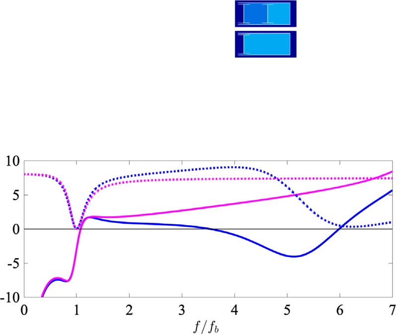
M.E. D’Elia et al.: Acta Acustica 2021, 5, 31                                              5

           (a)                                                                                                      7 mm
                                                                                                             l2 =
                                                                                                    9 mm                   12 mm
                                                                                             l1 =
                                                                                      2 mm
                                                                               2 mm                            1mm

                                                                             1mm
                                                                                                       (a)
           (b)

                                                                                                       (b)
Figure 4. (a) Absorption coefficient and (b) impedance as a
function of the normalized frequency when one (mono-articu-       Figure 5. (a) First (f = 709 Hz) and (b) second (f = 4412 Hz)
lated beam, in magenta) or two (bi-articulated beam, in blue)     mode of the cantilever beam with the I-cut shaped slits, as
modes are considered. For the first mode, the parameters are the   computed using a finite elements method (Comsol). l 1 and l 2 are
same that in Figure 2. The second mode is defined by               the lengths of the two parts of the beam.
xb2 = 6.05 xb, kb2eb2 = kbeb/8 and d2 = 2.5d.

Poisson’s ratio (which does not have a great influence on
the vibration of the beam) is estimated to be 0.35. The
Young’s modulus was adjusted to a value of 75 GPa so that
the first calculated resonance frequency corresponded to the
measured value.
    Two samples have been made: one for measurements in
a normal incidence tube (cut in a disk of diameter 38 mm)
and a second one for measurements in the wall of a rectan-
gular duct (cut in a rectangular plate of 120  50 mm2). For
these two samples, the micro-cutting was performed in the
                                                                  Figure 6. Schematic diagram of the setup for impedance tube
same way and with the same geometry. The micro-slits              experiments. Acoustic measurements are performed using four
were made by laser micro-cutting with high precision              microphones separated by distances L1. . .4). Vibrations are
machining. The resulting micro-slits are 50 lm wide (see          evaluated using a Laser Doppler vibrometer, and two measure-
inset pictures of Fig. 6).                                        ment points are defined on the beam. The back cavity of length
    Using the geometry and the material parameters and            B can be removed to characterize the blade alone. The inset
neglecting air loading on the beam, the vibration modes           pictures display the composite sample used for the normal
of the beam can be computed using a finite element method          incidence measurements, as well as a zoom on the laser cut slits.
(COMSOL). The first two vibration modes are shown in
Figure 5. The first one (f = 709 Hz, see Fig. 5a) corresponds      between the first microphone and the sample is
to an almost pure rotation of the whole beam. The stiffness       L1 = 230 mm. In order to measure the velocity induced
results from the deformation of the two arms at the base of       by the beam vibration, a laser vibrometer impinges on the
the beam. The second mode (f = 4412 Hz, see Fig. 5b) is a         beam. After an in-situ calibration of the microphones, the
bending mode while the third mode (f = 4453 Hz) is a tor-         signals from the microphones and from the laser vibrometer
sion mode which has an average velocity equal to 0. There-        are transferred to a data acquisition system. The measure-
fore, it is assumed not to interfere with the acoustics.          ments are performed using a sine sweep excitation signal
                                                                  going from 100 to 4000 Hz with a step of 5 Hz. At each fre-
3.1 Normal incidence measurements                                 quency, all transfer functions are averaged over 500 cycles.
                                                                      The measurement system allows to control the acoustic
   The circular sample is glued onto a ring (inner diameter       level of the incident wave. Several levels ranging from
30 mm, outer diameter 38 mm) and placed in an impedance           110 dB to 140 dB were tested but no non-linear effects were
tube which is made of steel tubes with an inner diameter of       detected.
30 mm and a wall thickness of 4 mm, see Figure 6. Four
microphones (B&K 4136 and 2670 with amplifier Nexus                3.1.1 Vibrometer measurements
2690) are used for the overdetermined separation of inci-
dent and reflected waves [24, 25]. The microphones are dis-           First, the velocity of the bi-articulated beam when
tant of L2 = 30 mm, L3 = 100 mm and L4 = 285 mm in                placed at the end of the tube (without cavity) was mea-
order to cover a large range of frequencies. The length           sured using a laser vibrometer, when acoustic excitation is
6 M.E. D’Elia et al.: Acta Acustica 2021, 5, 31
present. From the sound pressures measured on the three
microphones, it is possible to calculate the sound pressure
pi that is applied to the plate. The velocities vM 1 and vM 2
measured respectively at the end and in the middle of the
beam (i.e. at the end of the first plate composing the beam,
see Fig. 6 where the points M1 and M2 are indicated) related
to the incident pressure are plotted in Figure 7. The first
two modes of the bi-articulated plate can be seen very
clearly. The first mode is at a frequency of 710 Hz. For this
mode, we find that vM 1 =ðl1 þ l2 Þ ¼ vM 2 =l2 (l1 and l2 are
defined in Fig. 5). It indicates that this mode is very close
to a rotation of the plate around its base articulation, with- Figure 7. Dimensionless ratio between the velocities v M 1 and
out deformation. For the second mode (f = 3650 Hz), the v M 2 and the pressure on the plate pi. vb is the average velocity
velocities are almost opposite vM 1 ’ vM 2 , which indicates along the beam.
that we are dealing with a bending mode as shown in
Figure 5. An average velocity can be computed, assuming
two rigid plates pivoted to each other, by vb ¼ vM 2 =2þ frequency is f1 = 710 Hz. This difference comes from the
l1 vM 1 =ðl1 þ l2 Þ. This averaged velocity is also plotted in crudeness of the model used to predict stiffness. Neverthe-
Figure 7. Assuming a low radiation impedance of the tube less, this model allows us to identify the main parameters
and therefore zero sound pressure on the outside of the influencing this resonance frequency and to compare it with
plate, this average velocity relative to the sound pressure that of a cantilever beam of the same dimensions without
on the plate is the inverse of the impedance of the beam I-cuts, which is here given by x2 = 1.02(E/qb)e2/l4, leading
defined by equation (2): Zb = pi/(q0c0vb). to a frequency f = 2680 Hz. The structural damping is more
These velocity measurements confirm that the impe- complex to evaluate and is deduced from the vibrometer
dance Zb can be described by the contribution of the first measurements: d1 = 0.01.
two modes with: The values of the three parameters of the second mode
are deduced directly from the vibrometer measurements:
1 1 1 d2 = 1.25, A2 = 150, f2 = 3730 Hz. The measured impe-
¼ þ ;
Z b Z b1 Z b2 dance Zb (in blue) and the calculated impedance (in red)
are shown in Figure 8. A correct agreement between these
where two values is found, especially in the vicinity of resonances
2 ! where the imaginary part of Zb becomes zero.
f f1
Z b1 ¼ j A1 1 þ d1 ;
f1 f
3.1.2 Acoustic measurements
2 ! Using the four microphones described in Figure 6, the
f f2 reflection coefficient r can be obtained by an over-
Z b2 ¼ j A2 1 þ d2 :
f2 f determined separation of incident and reflected waves by
means of a least-squares method. From r, the absorption
Thus, this vibration measurement allows to experimentally coefficient a = 1 |r|2 and the impedance Z = (1 + r)/
determine some parameters of the model described in (1 r) can be easily computed. Here, the bi-articulated
Section 2. beam is backed up by a 30 mm deep closed cavity whose
Indeed, if some of them are easily computable such as the cross-section is as large as the incident tube (diameter
equivalent mass of the beam for the first mode, others are 30 mm).
more difficult to evaluate. From eq. (2), the equivalent mass To predict the impedance of this device, equation (5) is
is computed from A1 ¼ k b eb ¼ 4qb xb e=ð3q0 c0 Þ ¼ 10:55. used. In this equation, the beam impedance Zb is deduced
Note that the equivalent thickness of the beam is from the vibration measurements described in the previous
eb = 0.81 m. It corresponds to the thickness of air that would subsection. The cavity impedance Zc can be computed from
have to be set in motion to obtain the same effect. This equation (4) with B = 30 mm. The most tricky part to esti-
shows the interest of making vibrate a solid part when we mate is the acoustic impedance of the slit Zs. Indeed, the slit
want to perform low frequency attenuation. If we simply resistance is extremely sensitive to the width of the slit s. If
consider that the beam is a rotating plate and that the stiff- we use the relation Rs = 12le/(q0c0s2) we see that this resis-
ness comes from the deformation of the two arms of width tance is inversely proportional to the square of s. In addition
b = 1 mm and length a = 4 mm at the base of the plate, if one relates this impedance to the incident surface R = Si/
the resonance frequency reads x21 ¼ 0:5ðE=qb Þbe2 =ðBal3 Þ Ss Rs, where Si = lss and ls = 88 mm the total length of the
where E is the Young modulus, B is the width of the plate slits, we see that the resistance R is proportional to s3).
and l = l1 + l2 is its length. Using the dimensions and char- The machining process of these micro-slits results in a slight
acteristics of the cut composite plate, the predicted fre- conicity of the slit which therefore does not have a constant
quency is equal to f1 = 1080 Hz while the measured width s. On the height of e = 500 lm, it is estimated thatM.E. D’Elia et al.: Acta Acustica 2021, 5, 31 7
(a)
(b)
Figure 8. Impedance of the beam Zb deduced from the laser
vibrometer measurements. The blue curves are the measure-
ments and the red ones correspond to the fit described in the
text.
the width goes from 50 lm (see the photo under the micro-
scope on Fig. 6) at the narrowest to 100 lm on the other
side of the plate. For a constant width s = 50 lm the resis-
tance is R = 16 while for s = 100 lm the resistance is R = 2.
It is therefore difficult to say more than 2 < R < 16 and the Figure 9. (a) Absorption coefficient and (b) impedance as
exact value of R had to be experimentally adjusted. functions of the frequency. The resistance are displayed by
The measured absorption coefficient a and impedance Z dashed lines and the reactance by solid lines. The experimental
are plotted with a wide blue line in Figure 9. What happens results (blue curves) are compared to the analytical results
on these curves in the vicinity of the first resonance fre- computed with the bi-articulated plate model (red curves).
quency of the beam is very similar to what the model pre-
dicts. In particular, we can see that the maximum
absorption frequency (735 Hz) is slightly higher than the downstream of the test section. A sinusoidal sweep ranging
first resonance frequency of the beam (710 Hz) which in fact from 200 Hz to 4000 Hz with a step of 5 Hz is used.
corresponds to a very low absorption. We also note that the The sound pressure in the duct is recorded by two sets
real part of the impedance (dashed line in Fig. 9b) tends at of three flush-mounted microphones located upstream (ui)
low frequency towards a constant which is the resistance R. and downstream (di) of the test section, where i = 1 indi-
We can therefore estimate the value of the resistance: cates the microphone located the closest to the test section.
R = 8.5. The positions of the microphones are xu1 xu2 ¼ xd 2
At this stage, all the parameters that describe the mea- xd 1 ¼ 30 mm, xu1 xu3 ¼ xd 3 xd 1 ¼ 175 mm, and both
sured device are known and the impedance and absorption u1 and d1 are placed 113 mm away from the sample. All
coefficient can be calculated (thin red curve on Fig. 9). This the microphones are calibrated relatively to u1 in a separate
suggests that the proposed model takes into account the cavity. At each frequency step of the sine sweep, the acous-
main effects that occur in such a device and that it is pos- tic pressure on each microphone is calculated by averaging
sible to tailor such a system for specific uses. the pressure value over 400 cycles without flow, and over
1000 cycles with flow.
3.2 Grazing incidence measurements An overestimated determination of the incident and of
the reflected waves on both sides of the sample is permitted
In order to perform measurements with grazing inci- by this mounting of six microphones. Then, the elements of
dence and grazing flow, a second sample was made from the sample scattering matrix, namely the reflection and
the same composite material plate and with exactly the transmission coefficients (r±, t±) defined for incident plane
same micro-cutting geometry. This sample is made in a waves coming from upstream (r+, t+) and downstream
plate of 120 50 mm2, where 3 rows of 5 beams have been (r, t) of the sample, are computed. Two different acoustic
micro-cut, in blue on Figure 10. This plate was glued on a states are needed to obtain these four coefficients. The first
support (in black in Fig. 10) with 15 cavities of section one consists in placing the compression chambers upstream
15 22 mm2 and height B = 30 mm. of the test section, while they are located downstream for
During the measurements, this sample of 15 beams is the second acoustic state [28].
flush mounted on the wall of a waveguide with a rectangu- As for the normal incidence case, this measuring system
lar section. The height of the channel is H = 40 mm while makes it possible to control the acoustic level of the incident
the transverse dimension is 50 mm. This means that the wave. Several levels were tested but no non-linear effects
sample covers the entire width of the channel. This duct were detected.
facility has already been introduced and described in [26, To predict the effect of the sample on propagation, two
27]. The acoustic waves are generated by two compression separate actions are required. The first one is to calculate
chambers which can be placed either upstream or either the equivalent impedance of the sample. The second one8 M.E. D’Elia et al.: Acta Acustica 2021, 5, 31
t
t+
r
t
r
r+
Figure 11. Transmission and reflection coefficients of the liner
sample as a function of the frequency, without flow. The
Figure 10. (Top) Schematic representation of the grazing
experimental results (red curves) are compared to the results
incidence facility used to characterise the liner sample using two
provided by the multimodal method (green curves). For the
sets of three microphones. The duct has a rectangular cross
latter, the boundary condition in the lined section is given by the
section of height H ¼ 4 cm and a rotating lobe blower is used to
bi-articulated plate model.
introduce flow. (Bottom) The composite plate has been glued
over 15 cavities of section 15 22 mm2 so that there is one
cantilever beam per cavity. The height of the cavities is B ¼ 30
mm. and measured values of transmission and reflection is rela-
tively correct around the first resonance of the beam. It
can be noted that the hypothesis that one can substitute
is to predict the propagation in the duct in the presence of a discrete set of cells, of fairly large size, with a distributed
an acoustically treated wall. and homogeneous impedance can quickly find its limit when
The prediction of impedance is relatively easy since the the frequency increases. Moreover, the implicit assumption
impedances of the beam Zb and the slits Zs are identical to that cells do not acoustically interfere with each other is
the case in normal incidence since the material and the also very questionable.
geometry are the same. Similarly, since the cavity has the A striking effect is the disappearance of the second high-
same depth B, the cavity impedance Zc is also unchanged. frequency peak (near f2 = 3730 Hz). As f = 4000 Hz corre-
The only things that change in equation (5) are the incident sponds to the cut-off frequency of the second propagative
sections Si = 120 50/15 mm2 and the cavity section mode in the rigid conduit that our setup does not allow
Sc = 15 22 mm2. to characterize, it was not possible to know if this second
To predict the propagation with an impedance wall, a peak was rejected at higher frequency or if it simply disap-
numerical simulation is carried out. To this end, a multi- peared. As mentioned above, for these frequencies the
modal method is used to calculate the linearized two- length of a cell is of the order of a quarter of the wavelength
dimensional lossless problem. This method has already been and the hypothesis of uniformity of impedance is no longer
described in detail elsewhere [28] and therefore only a few valid.
points are merely reported. The linear propagation of small In spite of its approximations, the impedance homoge-
perturbations can be described by the linearized Euler and nization model, as expressed from equation (8), gives good
continuity equations. The multimodal method is used and results at low frequencies and makes it possible to under-
the perturbations are therefore expressed as a linear combi- stand the main effects of treatments with vibrating articu-
nation of the acoustic transverse modes. These modes and lated plates and micro slits on the propagation and
wave numbers are computed on uniform segments using a reflection of the incident acoustic field.
finite difference method by discretizing the equations in
the transverse y-direction. Here, the modes must be calcu- 3.3 Effect of flow
lated in the rigid duct and in the lined part wall. The scat-
tering matrix of the sample is found by matching the modes The implementation of the acoustic treatment in the
at the discontinuities at each ends of the sample. wall of a duct allows studying the effect of a flow on its
The comparison between the predicted and mea- acoustic behavior. For this purpose, the duct installation
sured transmission and reflection coefficient is depicted in is connected to a rotating lobe blower that can provide a
Figure 11. Due to reciprocity, without flow, the measured mean velocity of up to 85 m/s. The flow velocity is mea-
transmission coefficients in both directions are identical. sured at the center of the duct downstream of the test sec-
Conversely, the reflection coefficients r+ and r differ tion by a Pitot tube connected to a differential pressure
slightly. This seems to indicate some inhomogeneity sensor. This measurement gives the maximum value of
between the different beams which would not all react in the flow velocity in the duct section. It is then multiplied
the same way. This may for instance be due to the bonding by 0.8 in order to obtain the value of the average velocity
of the plate to its support, which may not be exactly iden- and the Mach number M [29]. The measurements shown
tical at every location. The comparison between predicted in Figure 12 were performed at a Mach number of 0.25.M.E. D’Elia et al.: Acta Acustica 2021, 5, 31 9
Acknowledgments
This research was supported by the European Union’s
Horizon 2020 research and innovation programme under
the Marie Skłodowska-Curie grant agreement No. 722401
With flow
t
(“SmartAnswer”) (https://www.h2020-smartanswer.eu/). The
No flow authors would like to thank Matthieu Giraud from Airbus
Against the flow Technocentre in Nantes for kindly supplying the compos-
ite plates.
Conflict of interest
Figure 12. Transmission coefficients of the lined sample in
presence of flow (M = 0.25). The experimental results (red The authors declare that they do not have any conflict
curves without flow, blue curves with flow) are compared to the of interst.
multimodal calculation (only the results with flow are shown,
cyan curves).
References
The presence of an assumed uniform flow is also fairly
easy to take into account in propagation modeling. To do 1. A. Guess: Calculation of perforated plate liner parameters
from specified acoustic resistance and reactance. Journal of
this, it is necessary to add convection terms to the equations Sound and Vibration 40 (1975) 119–137.
used. It is also necessary to modify the boundary condition 2. D.-Y. Maa: Potential of microperforated panel absorber. The
that applies to the wall with impedance. Here we have used Journal of the Acoustical Society of America 104 (1998)
the classical condition of continuity of pressure and normal 2861–2866.
displacement, in general referred as the Ingard [30] – Myers 3. M. Yang, S. Chen, C. Fu, P. Sheng: Optimal sound-
[31] condition [32]. Finally, it is necessary to apply a special absorbing structures. Materials Horizons 4 (2017) 673–680.
mode matching between the duct with impedance and the 4. Y. Wu, M. Yang, P. Sheng: Perspective: Acoustic metama-
terials in transition. Journal of Applied Physics 123 (2018)
rigid duct that takes into account this Ingard–Myers condi- 090901.
tion [28]. 5. B. Assouar, B. Liang, Y. Wu, Y. Li, J.-C. Cheng, Y. Jing:
The fairly good agreement between the experimental Acoustic metasurfaces. Nature Reviews Materials 1 (2018)
and the numerical results shows that the flow does not sig- 467–470.
nificantly change the value of the impedance of the mate- 6. X. Cai, Q. Guo, G. Hu, J. Yang: Ultrathin low-frequency
rial. The flow is therefore mainly introducing convection sound absorbing panels based on coplanar spiral tubes or
coplanar Helmholtz resonators. Applied Physics Letters 105
effects, both in the propagation itself and in the Ingard–
(2014) 121901.
Myers condition. 7. C. Chen, Z. Du, G. Hu, J. Yang: A low-frequency sound
absorbing material with subwavelength thickness. Applied
Physics Letters 110 (2017) 221903.
4 Conclusion 8. Y. Wang, H. Zhao, H. Yang, J. Zhong, J. Wen: A space-coiled
acoustic metamaterial with tunable low-frequency sound
This paper shows that it is possible and interesting to absorption. EPL (Europhysics Letters) 120 (2018) 54001.
use vibrating articulated plates combined with micro slits 9. S. Huang, X. Fang, X. Wang, B. Assouar, Q. Cheng, Y. Li:
Acoustic perfect absorbers via Helmholtz resonators with
to obtain sound attenuation at low frequencies. Two behav-
embedded apertures. The Journal of the Acoustical Society of
iors exist in this type of structure. In the first one, the America 145 (2019) 254–262.
frequency is closed to the structure alone resonance. In 10. J.-P. Groby, W. Huang, A. Lardeau, Y. Aurégan: The use of
the second one, only the structural mass is involved, the slow waves to design simple sound absorbing materials.
stiffness being provided by the cavity. In this second case, Journal of Applied Physics 117 (2015) 124903.
not studied in this paper [22], the frequency is higher for 11. Y. Aurégan, M. Farooqui, J.-P. Groby: Low frequency sound
a given height of the cavity. A very simple model has been attenuation in a flow duct using a thin slow sound material.
The Journal of the Acoustical Society of America 139 (2016)
developed to describe the behavior of this type of structure EL149–EL153.
both in normal and grazing incidence and fits well with the 12. F. Simon: Long elastic open neck acoustic resonator for low
experiments. Compared to other types of acoustic surfaces frequency absorption. Journal of Sound and Vibration 421
[11], this type of structure does not seem to be very sensitive (2018) 1–16.
to the effects of sound level and grazing flow, with the latter 13. W. Frommhold, H. Fuchs, S. Sheng, Acoustic performance of
being restricted to the convective effects on propagation. membrane absorbers, Journal of Sound and Vibration 170
Certainly, the operation of hinged plates with micro slits (1994) 621–636.
14. L. Huang: Modal analysis of a drumlike silencer. The Journal
is rather narrow-band and fatigue problems can occur when of the Acoustical Society of America 112 (2002) 2014–2025.
using vibrating parts, but this device can tackle low fre- 15. G. Ma, M. Yang, S. Xiao, Z. Yang, P. Sheng: Acoustic
quency noise in parallel with other devices for other fre- metasurface with hybrid resonances. Nature Materials 13
quency ranges. (2014) 873.10 M.E. D’Elia et al.: Acta Acustica 2021, 5, 31
16. M. Yang, P. Sheng: Sound absorption structures: From 24. M. Åbom: Measurement of the scattering-matrix of acousti-
porous media to acoustic metamaterials, Annual Review of cal two-ports. Mechanical Systems and Signal Processing 5
Materials Research 47 (2017) 83–114. (1991) 89–104.
17. Y. Aurégan: Ultra-thin low frequency perfect sound absorber 25. M. Leroux, Y. Aurégan: Failures in the discrete models for
with high ratio of active area. Applied Physics Letters 113 flow duct with perforations: an experimental investigation,
(2018) 201904. 265 (2003) 109–121.
18. X. Dai, Y. Aurégan: Flexural instability and sound ampli- 26. M. D’Elia, T. Humbert, Y. Aurégan: Effect of flow on an
fication of a membrane-cavity configuration in shear flow. array of helmholtz resonators: Is kevlar a “magic layer”? The
The Journal of the Acoustical Society of America 142 (2017) Journal of the Acoustical Society of America 148 (2020)
1934–1942. 3392–3396.
19. H.K. Fan, R.C. Leung, G.C. Lam, Y. Aurégan, X. Dai: 27. M.E. d’Elia, T. Humbert, Y. Auregan, J. Golliard: Optical
Numerical coupling strategy for resolving in-duct elastic measurements of the linear sound-flow interaction above a
panel aeroacoustic/structural interaction. AIAA Journal 56 corrugated plate, in 25th AIAA/CEAS Aeroacoustics Con-
(2018) 5033–5040. ference, 2019, 2716.
20. E. Martincic, A. Houdouin, S. Durand, N. Yaakoubi, E. 28. Y. Aurégan, M. Leroux, V. Pagneux: Measurement of liner
Lefeuvre, Y. Aurégan: Acoustic absorber, acoustic wall and impedance with flow by an inverse method, in 10th AIAA/
method for design and production (2019) US Patent CEAS Aeroacoustics Conference, 2004, 2838.
10,477,302. 29. H. Schlichting: Boundary layer theory. 7th ed. McGraw-Hill,
21. M. Farooqui, Y. Aurégan: Compact beam liners for low New York, 1979.
frequency noise, in 2018 AIAA/CEAS Aeroacoustics 30. U. Ingard: Influence of fluid motion past a plane boundary on
Conference, 2018, 4101. sound reflection, absorption, and transmission. The Journal
22. Y. Aurégan, M. Farooqui: In-parallel resonators to increase of the Acoustical Society of America 31 (1959) 1035–1036.
the absorption of subwavelength acoustic absorbers in the 31. M. Myers: On the acoustic boundary condition in the presence
mid-frequency range. Scientific Reports 9 (2019) 1–6. of flow. Journal of Sound and Vibration 71 (1980) 429–434.
23. J.-F. Allard, N. Atalla: Propagation of sound in porous 32. Y. Renou, Y. Aurégan: Failure of the Ingard–Myers boundary
media: modelling sound absorbing materials 2e. John Wiley condition for a lined duct: an experimental investigation, The
& Sons, 2009. Journal of the Acoustical Society of America 130 (2011) 52–60.
Cite this article as: D’Elia M.E. Humbert T. & Aurégan Y. 2021. On articulated plates with micro-slits to tackle low-frequency
noise. Acta Acustica, 5, 31.You can also read