Dictionary Learning for Image Style Transfer - Harvard DASH
←
→
Page content transcription
If your browser does not render page correctly, please read the page content below
Dictionary Learning for
                     Image Style Transfer
                  The Harvard community has made this
               article openly available. Please share how
               this access benefits you. Your story matters

Citation              Seo, Hyeon-Jae. 2020. Dictionary Learning for Image Style Transfer.
                      Bachelor's thesis, Harvard College.

Citable link          https://nrs.harvard.edu/URN-3:HUL.INSTREPOS:37364670

Terms of Use          This article was downloaded from Harvard University’s DASH
                      repository, and is made available under the terms and conditions
                      applicable to Other Posted Material, as set forth at http://
                      nrs.harvard.edu/urn-3:HUL.InstRepos:dash.current.terms-of-
                      use#LAA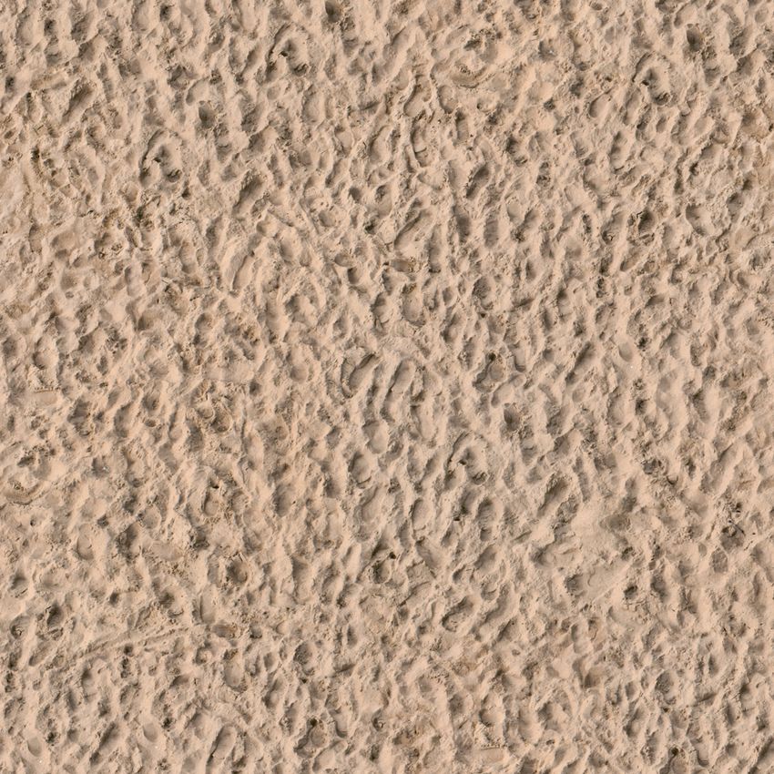
Dictionary Learning for Image Style Transfer

                         Hyeon-Jae Seo
              Supervised by Prof. Demba Ba

          Presented to the Department of Applied Mathematics
                 in partial fulfillment of the requirements
                for a Bachelor of Arts degree with Honors

                        Harvard University
                      Cambridge, Massachusetts

                            April 3, 2020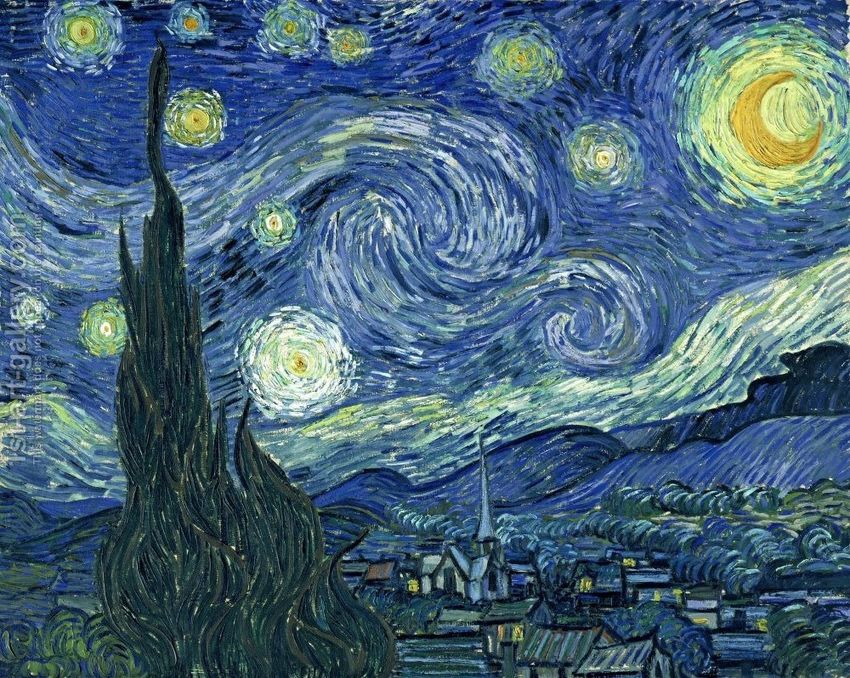
Abstract

    Deep image representations learned by CNNs have been shown to successfully separate image content
from style, but the generic feature representations learned by CNNs are far from interpretable. Drawing
upon recent developments in neural network inspired extensions of Dictionary Learning (DL) to multi-
layer models, I present a framework using dictionary learning and sparse code representations to separate
image content and style in natural images. This framework provides an interpretable decomposition
of images into high and low frequency representations that can be used to generate new images by
combining the style and content of any two arbitrary images. These decompositions and visualizations of
convolutional filters provide novel insights into the image representations learned by convolutional neural
networks and demonstrate the potential of DL and sparse code representations for image analysis and
transformation.

                                                    1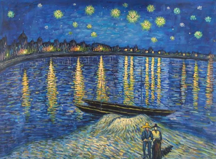
Contents

1 Introduction                                                                                                      3
  1.1   Related Work . . . . . . . . . . . . . . . . . . . . . . . . . . . . . . . . . . . . . . . . . . . . .      3
  1.2   Problem Specification . . . . . . . . . . . . . . . . . . . . . . . . . . . . . . . . . . . . . . . .       4
        1.2.1   Motivating Example . . . . . . . . . . . . . . . . . . . . . . . . . . . . . . . . . . . . .        4
  1.3   Overview of Thesis . . . . . . . . . . . . . . . . . . . . . . . . . . . . . . . . . . . . . . . . . .      4

2 Background                                                                                                        5
  2.1   A Generative Model of Images . . . . . . . . . . . . . . . . . . . . . . . . . . . . . . . . . . .          5
  2.2   Convolutional Sparse Coding . . . . . . . . . . . . . . . . . . . . . . . . . . . . . . . . . . . .         6
  2.3   Hierarchical CSC for Image Encodings . . . . . . . . . . . . . . . . . . . . . . . . . . . . . . .          6
  2.4   Proximal Algorithms . . . . . . . . . . . . . . . . . . . . . . . . . . . . . . . . . . . . . . . . .       6
        2.4.1   FISTA . . . . . . . . . . . . . . . . . . . . . . . . . . . . . . . . . . . . . . . . . . . . .     7
  2.5   Convolutional Dictionary Learning . . . . . . . . . . . . . . . . . . . . . . . . . . . . . . . . .         8

3 Model                                                                                                             9
  3.1   Notation . . . . . . . . . . . . . . . . . . . . . . . . . . . . . . . . . . . . . . . . . . . . . . . .    9
  3.2   Implementation . . . . . . . . . . . . . . . . . . . . . . . . . . . . . . . . . . . . . . . . . . . .      9

4 Simulations                                                                                                      10
  4.1   Image Data Generation . . . . . . . . . . . . . . . . . . . . . . . . . . . . . . . . . . . . . . .        10
  4.2   Dictionary Learning . . . . . . . . . . . . . . . . . . . . . . . . . . . . . . . . . . . . . . . . .      11

5 Experimental Results                                                                                             14
  5.1   Style Transfer . . . . . . . . . . . . . . . . . . . . . . . . . . . . . . . . . . . . . . . . . . . . .   15

6 Conclusion                                                                                                       17

7 Acknowledgements                                                                                                 18

                                                         2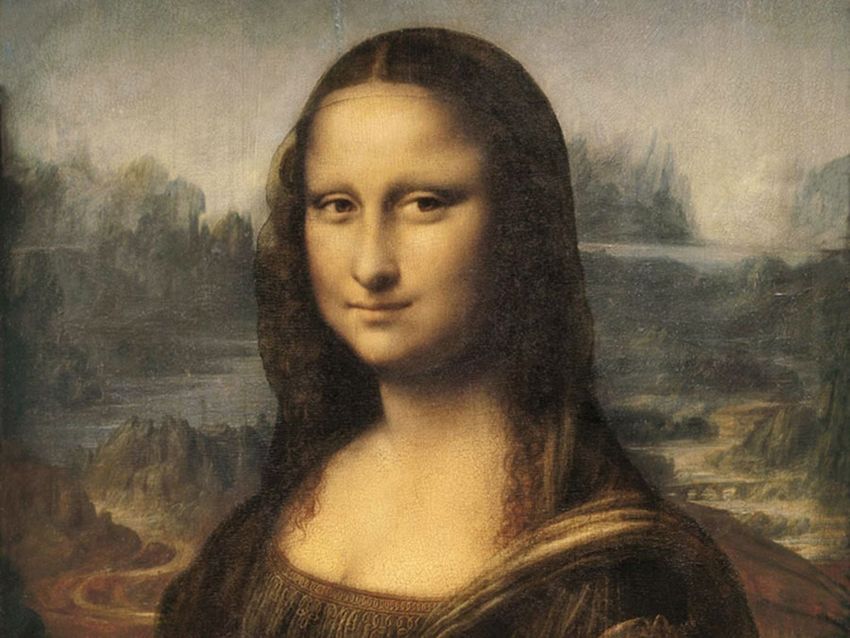
1     Introduction

Advancements in deep learning and convolutional neural networks (CNNs) present a significant paradigm
shift in the landscape of automated image style transfer, in which the semantic content of an image is
rendered in a different style. Deep CNNs have demonstrated the capability to perform neural style transfer
(NST) between arbitrary images [7], which entails training a deep neural network to generate artistic images
by combining the content and style of arbitrary images. Thus, deep learning provides the potential for
broad-ranging and flexible style transfers, but CNN-based approaches are computationally expensive due to
the heavy optimization involved in obtaining synthesized images close to the content image. Furthermore,
the challenge of interpreting the style representations learned by CNNs persists.
In this work, I present a novel framework to address both of these issues that draws upon the theory of wavelet
analysis and dictionary learning. Representation analysis with wavelets is a classical, interpretable, and well
understood theory that allows us to decompose images/signals into a linear combination of basis functions
at different scales to represent an image and recover it perfectly via convolution operations [13, 12], while
sparse coding (SC) [1] finds sparse representations of images, or signals more broadly. Thus, wavelet analysis
and sparse coding provide a way to decompose images into distinct style and content representations, while
dictionary learning provides a framework for learning the shared structure of images. I call this framework
a hierarchical generative model for image analysis and show that this model learns visually interpretable
convolutional filters and highly efficient representations of images that can very faithfully reconstruct even
complex colored images.
The challenges regarding the computational complexity and limited interpretability of CNNs are of great
importance due to the widespread use of CNNs. Reducing the dependence on exceptionally large compu-
tational resources would diminish the financial and environmental impact of training and developing CNN
based models [17], while obtaining more efficient and interpretable representations from CNNs would help
ease the adoption of such models in new application areas. While in this work we focus on a specific use
case in the artistic domain, a more detailed and nuanced understandings of the role of convolutions in image
style transfer would have great significance in the fields of computer graphics, vision, and image processing
more broadly.

1.1    Related Work

The diverse literature on image style transfer has its roots in the simpler task of texture synthesis, in which
the goal is to synthesize a new texture that appears to have been generated via the same process as a
given texture sample. Several techniques, including physical simulation of their generation process [3, 20,
21], Markov random fields with Gibbs sampling [5, 14, 15], and feature matching [2, 8, 16], have all been
successfully applied towards this task.
These developments were followed by demonstrations of texture transfer via techniques like image quilting
[10], image analogies [9], and extensions of texture synthesis algorithms to account for content similarities
[6]. On the machine learning front, several attempts have been made to develop a feedforward style transfer
network that is trained to go from a content image to a stylized image in one pass [19, 11]. Yet a significant
drawback of these style transfer networks is that they are tied to the single style on which they are trained,
which means separate networks need to be trained for each style modeled. Dumoulin et al. (2017) tackled this
issue by introducing conditional instance normalization, in which a single conditional style transfer network
is trained on multiple styles, and while each specific style uses specialized parameters, the convolutional
weights are share across all styles. This extension allows style transfer networks to learn multiple styles
while still maintaining both the qualitative and convergence properties of the single-style transfer networks.

                                                      3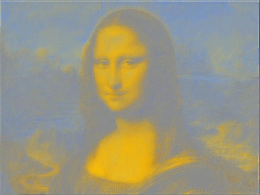
1.2 Problem Specification
Given two datasets Ds and Dt of images in styles s and t, respectively, our question is twofold. First, can
we separately capture style or texture and content information in images with representation analysis? I
show that the latent representations learned by the hierarchical generative model presented here does indeed
capture image specific texture and content details, while the convolutional filters capture common structural
information that is shared across images in a given dataset. Here, the term ”image texture” refers to the
spatial arrangement of colors or intensities in a given image. This is the first primary contribution of this
project – while previous work in this area has looked at the role of shared filters in convolutional neural
networks for style transfer, to my knowledge this is the first attempt to obtain interpretable decompositions
of an image into style and content representations.
Second, can we synthesize new images by arbitrarily combining the content of one image with the style of
another? Although measures of style are not quantitatively defined, we can assess the extent to which the
style and content aspects of the source images are transferred to the target image through visual inspection.
The second major contribution of this work is a demonstration of arbitrary style transfer using the set of
filters learned by the hierarchical generative model with no additional training.
1.2.1 Motivating Example
To illustrate the task at hand, consider the following setting. I have a photographic portrait of a woman, as
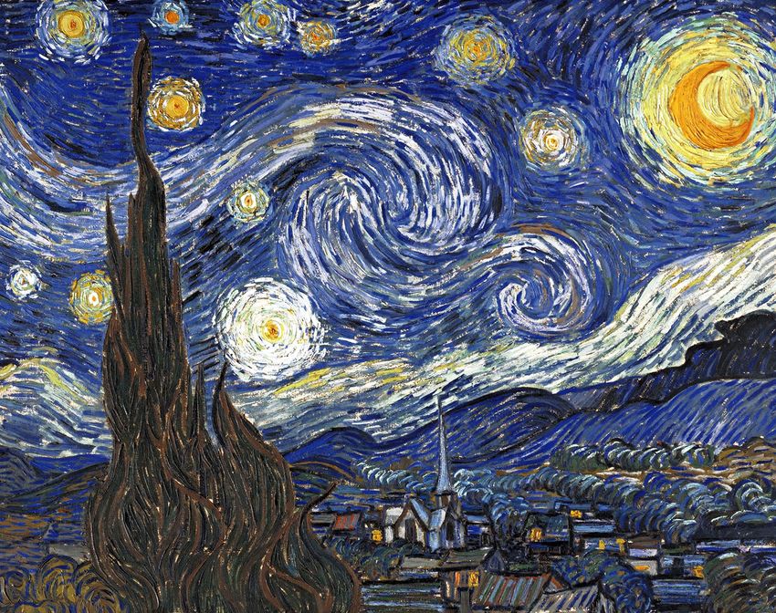
in Fig 1(a), and a copy of Vincent Van Gogh’s Starry Night, as in Fig 1(b). I would like to synthesize a new
image featuring the woman in the portrait but in the style of Van Gogh’s painting. One possible rendition
of such a transfer can be seen in Fig 1, which was generated by [4] using a deep neural network. My goal is
to attempt a similar task but with the proposed hierarchical generative model instead of a neural network,
while maintaining generality so that we can conduct such a style transfer between any two arbitrary images
of the selected styles.
(a) Photographic portrait of a (b) Vincent Van Gogh’s Starry (c) Newly generated image com-
woman (from Dumoulin et al. Night bining content from (a) with the
2017) style from (b) (also from Du-
moulin et al. 2017)
Figure 1: Motivating example of style transfer
1.3 Overview of Thesis
The remainder of this thesis is organized as follows. Section 2 provides the background on the technical
concepts that are drawn upon in this project and section 3 specifies the model used. Section 4 details
the simulations used to develop intuition for the application of the hierarchical generative model for image
analysis, while section 5 presents the results of experiments conducted on natural images. Section 5 concludes.
4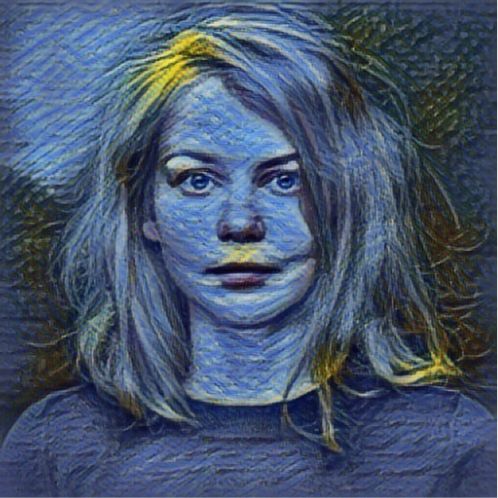
2     Background

2.1    A Generative Model of Images

Given a dense signal xL and the sparse signals u = [u1 , . . . , uL ], I can define the following recursive generative
model proposed by [22]

                                 x`−1 = A` ∗ x` + B` ∗ u` + ` ,           ` ∈ {1, . . . , L}                     (1)

Here ` indicates the layer the signals correspond to, where ` = 0 represents the input image and ` > 0
denotes deeper layers, with a total depth of L. Throughout this manuscript, I will interchangeably refer
to x` and u` as signals, encodings, and latent representations. A` and B` represent texture and content
filters, respectively. Filters are tensors of dimension C` × D` × H` × W` , denoting the number of output
channels, number of input channels, filter height, and filter width, respectively. The ∗ operation denotes a
full convolution between a filter and a signal, which is more explicitly defined by the following
                                                  D
                                                  X̀
                                (A` ∗ x` )(c) =         A` (c, d) ∗ x` (d), ∀c ∈ 1, . . . , C`                    (2)
                                                  d=1

where c indexes the output channels and d indexes the input channels. Throughout this manuscript, the
convolution between A and x, here denoted as A ∗ x, may be shortened to just Ax when it is clear that this
operation denotes a convolution.
Furthermore, we assume the following latent prior distributions:

                                                  u` ∼ Laplace(0, λ` )                                            (3)
                                                  x` ∼   N (0, σx2` )                                             (4)

The Laplacian prior on u` supports its sparsity and facilitates the capture of high frequency information in
u` , while the Gaussian prior on x` supports a non-sparse form and facilitates the encoding of low frequency
information in x` . As textural information primarily takes the form of color and patterns, it presents a source
of low frequency information, whereas content information primarily entails edge detection, and therefore
presents high frequency information. Thus, A` and x` are intended to capture texture information, while
B` and u` are intended to capture content information.
Figure 2 depicts a graphical representation of the generative model defined by Eq. 1 for three layers. As the
sparse signals u` are independent across layers, the sparsity requirement does not impose restrictions on the
depth of the model and any depth is attainable.

                                 Figure 2: Hierarchical model representation for L = 3

In the following sections, I further specify the assumptions of this model and methods for finding the
encodings x` and u` .

                                                              5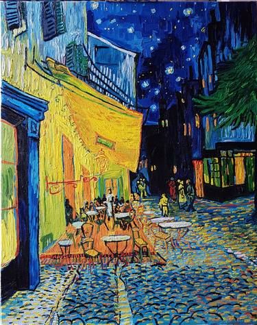
2.2     Convolutional Sparse Coding

While I can synthesize images given the signals xL and u = [u1 , . . . , uL ] following the generative model of
Eq 1, recovering these encodings from an input image x0 requires solving the inverse problem. This problem
has its roots in the theory of sparse coding, which refers to a class of algorithms for factoring input data
into a linear combination of over-complete basis vectors, B = [b1 , . . . , bK ]. A commonly used cost function
for this task is
                                                     N
                                                  1X
                                         min            kyn − Bun k22 + λkun k1
                                          B,u     2 n=1
                                   subject to kbk k22 ≤ 1 for k = 1, . . . K                                (5)

where λ controls the L1 regularizer and the constraints on bk ensure that the dictionary B doesn’t absorb all
magnitude-related information. This formulation is also commonly known as LASSO [18] and its usefulness
has been demonstrated in a variety of machine learning contexts.
One advantage of over-complete bases over complete bases is that the former are more conducive to capturing
structures and patterns in the data. However, traditional sparse coding assumes that the input vectors
{yn }N
     n=1 are independent, which leads to basis vectors that are translations of each other for natural images.
Convolutional sparse coding addresses this problem by incorporating shift invariance into the objective
function:
                                                          K                  K
                                                1      X                 X
                                      min         ky −   bk ∗ uk k22 + λ   kuk k1
                                      B,u       2
                                                         k=1                k=1
                                subject to kbk k22 ≤ 1 for k = 1, . . . K                                   (6)

Now, when bk ∗ uk is summed over all k, the result should approximate the full input signal y, rather than
independent sections, as would have resulted from the objective in Eq. 5.

2.3     Hierarchical CSC for Image Encodings

To recover the dense signals x` across layers in addition to the sparse codes, I need to solve a derivation
of the sparse coding coding problem developed by [22] and termed hierarchical convolutional sparse coding
(H-CSC). In this setting, an input image x0 is decomposed into both dense scale and sparse detail signal
components by solving the following problem

                            x̂` , û` = arg min f (x̂`−1 , x` , u` ) + λ` ku` k1 + γ` kx` k22               (7)
                                         x` ,u`

where
                                                        1
                               f (x̂`−1 , x` , u` ) =     kx̂`−1 − A` ∗ x` − B` ∗ u` k22                    (8)
                                                        2

for every ` ∈ {1, . . . , L}. Here, x̂0 = x0 is the given input image and subsequent estimates x̂` are obtained
by solving Eq. 7. The `1 -norm enforces sparsity on u` with the parameter λ controlling the level of sparsity.
Note that by setting A` = 0, we return to the traditional sparse coding setting of the previous section.

2.4     Proximal Algorithms

Because Eq. 7 is non-smooth and convex, it can be solved with a proximal gradient method, a common
framework for solving nonsmooth, constrained optimization problems of the form

                                                               6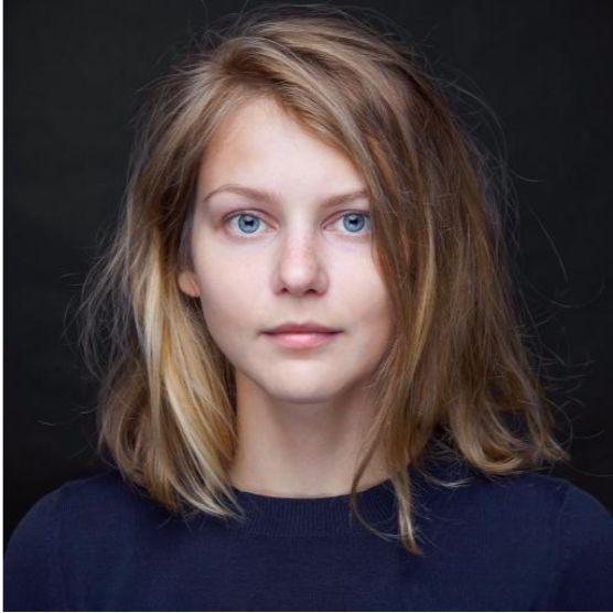
min f (x) + g(x)                                            (9)
                                                x

where both f and g are proper closed convex and f is differentiable. The non-smooth nature of g is handled
via a proximal operator, defined as


                                                            1
                                  proxg (y) = arg min g(x) + kx − yk22                                  (10)
                                                 x          2

where k · k2 is the Euclidean norm. This function is strongly convex and not everywhere infinite, so it has a
unique solution y ∈ RN . For a scaled function λg, where λ > 0, the corresponding proximal operator is


                                                             1
                                proxλg (y) = arg min g(x) +    kx − yk22                                (11)
                                                x           2λ

The proximal operator can be considered to be like a gradient step for g, as we have that

                                          proxλg (y) ≈ y − λ∆g(y)                                       (12)

Furthermore, proxλg (x∗ ) = x∗ if and only if x∗ minimizes g. I can therefore minimize g by finding a fixed
point of proxg . In particular, due to the firm nonexpansiveness property of proxg , the iterative proximal
method given by
                                             xk := proxλg (xk−1 )                                      (13)
converges to the set of minimizers of g, provided that g has a minimum. Here k denotes an iteration counter
and xk is the kth iteration of the algorithm. Returning to the motivating minimization problem, the basic
proximal gradient method to solve Eq. 9 is

                                     xk := proxλg xk−1 − λ∆f (xk−1 )

                                                                                                        (14)

By replacing the λ with λk , I can also handle
                                          P∞ parameter values that change in each iteration. Convergence
is still guaranteed as long as λk > 0 and k=1 λk = ∞.

2.4.1   FISTA

Adopting the idea behind the basic proximal gradient method presented in Eq. 14 to a nonsmooth regularized
problem of the form
                                             min f (x) + λkxk1                                        (15)
                                               x

the gradient iteration can be written as

                 k                 k−1            k−1         k−1      1        k−1 2
                x = arg min f (x       ) + hx − x     , ∆f (x     )i + k kx − x    k + λkxk1            (16)
                         x                                            2t

As I can drop constant terms and separate the l1 norm, this minimization reduces to solving

                                       xk = Tλtk (xk−1 − tk ∆f (xk−1 ))                                 (17)

where Tα : Rn → Rn is the shrinkage operator given by

                                         Tα (x) = (|x| − α)+ sgn(x)                                     (18)

                                                      7
The iterative scheme of Eq. 17 forms the basis of a popular proximal gradient method known as ISTA,
or Iterative Shrinkage-Thresholding Algorithm. This method has been extended to an accelerated version
known as FISTA, or the Fast Iterative Shrinkage-Thresholding Algorithm. This procedure is the one we use
and is outlined in Algorithm 1.
Algorithm 1 FISTA for H-CSC
1: Input: x` , α, λ` , γ`
2: Initialize: x1`+1 , u1`+1 , t1 = 1
3: for k ∈ {1, . . . , p
K} do
4: tk+1 ← 1 + 1 + 4(tk )2 /2
5: ū ← uk` + (tk − 1)(uk` − u`k−1 )/tk+1
6: x̄ ← xk` + (tk − 1)(xk` − x`k−1 )/tk+1
7: r ← A` ∗ x̄ + B` ∗ ū − x`
8: xk+1
` ← x̄ − α(r ? A` + γ` x̄)
k+1
9: u` ← Sλ` α (ū − α(r ? B` ))
10: end for
11: return xK ` , u`
K
2.5 Convolutional Dictionary Learning
I have now described how to recover the variables x` and u` across layers assuming the filters A` and B`
are fixed, so it remains to expound on the method for learning the filters A` and B` . To update the filters,
we fix x` and u` and minimize the following loss function:
N
X
min kx̂`−1,i − A` ∗ x̂`,i − B` ∗ û`,i k22 , s.t. A` ? A` = 1, B` ? B` = 1 (19)
A` ,B`
i=1
where x̂`,i , û`,i represents the estimates of the encodings at depth ` for the ith image in a dataset indexed
by {1, . . . , N }.
I can then update the filters by directly computing the first order gradient of Eq. 19. Since the filters are four
dimensional tensors (C` × D` × H` × W` ) whereas the images and intermediate signals are three dimensional
(D` × H` × W` ), we extend the dimension of the images by one and obtain the following gradients
∂
kx̂`−1,i − A` ∗ x̂`,i − B` ∗ û`,i k22 = (A` ∗ x̂`,i + B` ∗ u`,i − x̂`−1,i ) ∗ x̂`,i
∂A`
∂
kx̂`−1,i − A` ∗ x̂`,i − B` ∗ û`,i k22 = (A` ∗ x̂`,i + B` ∗ û`,i − x̂`−1,i ) ∗ u`,i (20)
∂B`
which are then used to update the filters A` and B` appropriately.
Given these methods for recovering both x̂` and û` assuming A` and B` are fixed, as well as for identifying
A` and B` assuming x̂` and û` are fixed, I can solve Eq. 1 by utilizing an optimization procedure that
alternates between these two methods. The following section specifies the framework used to combine these
methods.
83 Model
3.1 Notation
Notations and conventions used throughout this manuscript are summarized in Table 1.
Symbol Description
A Matrix (upper-case bold letter)
 Matrix learned by a model
x Vector (lower-case bold letter)
x̂ Estimation of vector x
x`,i Vector x corresponding to the `th layer of the ith data sample
xi Vector x corresponding to the ith data sample when the # of layers L = 1
xk Vector x at the k th iteration of an iterative algorithm
kxkp The `p -norm of vector x
∗ Linear convolution
2
N (µ, σ ) Gaussian distribution with mean µ and variance σ 2
Table 1: Notation and conventions
3.2 Implementation
To incorporate the methods described in the previous section into a cohesive method, I utilize an autoencoder
framework as follows:
1. The filters Â` and B̂` are initialized with values drawn from N (0, 1).
2. A batch of images, I, is drawn from the chosen dataset, D, and is fed into the network.
3. In the first half of the forward pass, the model uses FISTA to estimate the underlying signals x̂`,i and
û`,i for each image yi ∈ I and each layer ` ∈ {1, . . . , L}. This is commonly known as the encoding
step.
4. In the second half of the forward pass, the model reconstructs estimates of the input images, ŷi , from
the encodings x̂`,i and û`,i identified in the previous step following the recursive formula in Eq. 1.
This is commonly known as the decoding step.
5. In the backward pass, the loss function in Eq. 19 is used to measure the discrepancy between the original
images, yi , and the reconstructed images, ŷi , which is then used to update Â` and B̂` accordingly.
6. Steps 3 through 5 are repeated for the specified number of epochs, drawing a different batch from the
image dataset each time.
Note that the filters Â` and B̂` are shared across all images in the dataset, whereas the encodings x̂`,i and
û`,i are image specific.
The entire framework is created using PyTorch and relies heavily on the torchvision package for manipulating
images.
94 Simulations
To visually illustrate the hierarchical generative model framework, I generate some sample images and provide
intuition for the theory of style transfer in this context.
4.1 Image Data Generation
I focus on the 1 layer case with grayscale images (i.e. one input channel and one output channel), and thus to
simplify notation, I drop the subscripts on the filters and encodings that denote the layer of each component.
This means that the generation process for an image yi is defined as follows:
yi = Axi + Bui (21)
where A, B are the shared texture and content filters, respectively, and xi , ui are the image-specific texture
and content encodings, respectively. yi denotes the final image generated from a linear combination of these
components. Note that in this generation process, I am initializing the latent representations to synthesize
an image, whereas later I will be solving the reverse problem, i.e. decomposing a given image into its latent
representations.
To obtain A, I start with an arbitrarily selected colored texture image T (see Figure 3). I crop T to the
desired dimensions, which is 25 × 25 pixels in this case. I then convert the cropped image to grayscale, recast
it as a tensor, and normalize the values in the tensor.
(a) Marble (b) Sand
Figure 3: Sample close-up images of textures taken from an opensource database. (a) Marble (b) Sand
For B, I use an edge filter from the Leung-Malik (LM) filter bank, which consists of 48 derivatives of
Gaussians, providing a mix of edge, bar, and spot filters at multiple scales and orientations. For this
simulation I focus on a simple horizontal edge filter for visual clarity.
Next, I initialize ui and xi to two randomly generated sparse vectors. Figure 4 illustrates how A convolved
with the randomly generated x generates an image where A is precisely replicated at each non-zero location
in xi . Figure 5 illustrates the analogous process for the convolution of B and u.
(a) A (b) xi (c) A ∗ xi
Figure 4: Generative process for Axi . (a) Texture filter, A (b) Texture encoding, xi , where the white pixels represent the 5
non-zero values (c) The final product of a linear convolution, A ∗ xi
10(a) B (b) ui (c) B ∗ ui
Figure 5: Generative process for Bu. (a) Edge filter, B (b) Content signal, u, where the white pixels represent the three
non-zero values (c) The final product of a linear convolution, B ∗ ui
While xi is intended to be a relatively dense signal, for illustration purposes I keep xi sparse in this simulation
so its visual effect is more readily observed. As is seen in Figure 6, increasing the number of non-zero values
in xi leads to a visually incomprehensible overlapping of the texture filter. Here, n-sparse refers to a tensor
with n non-zero values. It appears that the effect of xi appears to be increasingly dominant in the convolution
as xi becomes less sparse. Thus initializing xi to a dense signal would lead to an image in which the values
of xi completely dominate the generated image.
(a) 5-sparse (b) 15-sparse (c) 50-sparse
Figure 6: Visualization of Axi for different sparsity levels of xi , using the same filter A. (a) 5-sparse (b) 15-sparse (c) 50-sparse
Once I have generated Axi and Bui , I perform a linear convolution to generate yi , presented in Figure 7.
As expected, yi looks like a superposition of the visualizations of Axi and Bui from Figures 4 and 5.
(a) Axi (b) Bui (c) yi = Axi + Bui
Figure 7: Generation of the image y through a linear combination of Ax and Bu.
Finally, I demonstrate a very rudimentary example of style transfer using this hierarchical generative frame-
work by taking advantage of the modularity of the model. Figure 8 shows that I can easily exchange A for
a different filter, A∗ , to change the appearance of the texture filter replicated at the locations determined
by xi , while the locations and appearance of the edge filter, B, remain exactly the same.
4.2 Dictionary Learning
Having illustrated the data generation process, I now demonstrate the applicability of FISTA and dictionary
learning on the simulated images. Again I stick to the one layer case and start by looking at the texture and
11(a) yi = Axi + Bui (b) A∗ (c) yi∗ = A∗ xi + Bui
Figure 8: Demonstration of style transfer, where only the texture filter, A, is changed to A∗ and B, ui , and xi are kept the
same
content components separately. First, I generate images using the yi = Axi framework with a 1 channel
texture filter of size 5 × 5 for A and a randomly generated vector for xi , resulting in an image of size
100 × 100. I generate a total of 1000 such sample images and pass these images through the autoencoder
framework in batches of 64 to learn both the filter and the signal. Here, I denote  as the filter estimated
through dictionary learning and x̂ as the signal estimated through FISTA. Further details regarding the
hyperparameters used for FISTA and dictionary learning are specified in Table 2. I verify that the model is
capable of recovering both of these components with reasonable accuracy, as can be seen in Figure 9.
(a) Original (b) Reconstruction
Figure 9: Comparison of the original Axi to its reconstruction, Âx̂i
(a) Original A (b) Random initialization of  (c)  after training
Figure 10: Comparison of the original texture filter, A, to the filter learned by the model, Â. (a) Original A (b) Random
Gaussian initialization of  (c)  after training for 150 epochs with a learning rate of 0.02
I repeat this process with the framework yi = Bui . I begin by generating images using a 5 × 5 edge filter
from the LM filter bank for B and a randomly generated vector for ui and pass the resulting images through
the model. As before, I generate a total of 1000 images of size 100 × 100, split into batches of size 64, and
use the same hyperparameters listed in Table 2. Again, I verify that the model recovers both the filter B
and the signal ui with high accuracy, as is seen in Figure 11.
Of particular significance is the extent to which the learned convolutional filters visually resemble the original
filters. While Figures 12(a) and 12(c) appear to be mirror images of one another, this merely demonstrates
the fact that the model is only concerned with reproducing the edges present in the input image, which may
lead to some variation in the learned filters.
12(a) Original (b) Reconstruction
Figure 11: Comparison of the original Bui to its reconstruction, B̂ûi
(a) Original (b) Randomly initialization of B̂ (c) B̂ after training
Figure 12: Comparison of the original edge filter, B, to the filter learned by the model, B̂. (a) Original B (b) Random Gaussian
initialization of B̂ (c) B̂ after training for 40 epochs with a learning rate of 0.02
Sparseness of code (kxi k0 and kui k0 ) 3
# layers L 1
# filter input channels Cin 1
# filter output channels Cout 1
Filter kernel size K 5
Dimensions of each sample D 100 × 100
# samples N 1000
Batch size B 64
# epochs 40
FISTA iterations T 200
FISTA learning rate α 2 × 10⁻³
FISTA regularizer λ 0.03
FISTA regularizer γ 0
Dictionary learning rate 0.02
Table 2: Details of datasets and training parameters for experiments on simulated data.
Thus, I have demonstrated that both the filters learned by the model and the encodings obtained through
FISTA are visually meaningful and interpretable, and also that the hiearchical image generation process
used in this section is highly intuitive.
135 Experimental Results
Having demonstrated the viability of the hierarchical generative framework and developed intuition for style
transfer using simulated images, I move to experimenting on natural images. Returning to our original
motivating application in the artistic domain, I train the hierarchical model on datasets of images generated
using paintings by historically prominent artists. To generate the first dataset, DV G , each of the three Van
Gogh paintings shown in Figure 13 are randomly cropped to 100 × 100 sized images 100 times, to generate
a dataset with a total of 300 image croppings (100 per painting). The filters learned from this dataset will
be referred to as ÂV G and B̂V G . To generate the second dataset, DM L , the Mona Lisa painting shown in
Figure 14 is similarly randomly cropped to 100 × 100 pixel sized images 100 times, to generate a dataset
with a total of 100 image croppings. The corresponding filters learned from this dataset will be referred to
as ÂM L and B̂M L .
(a) Starry Night (b) Cafe Terrace At Night (c) Starry Night Over The Rhone
Figure 13: Set of Vincent Van Gogh paintings used to generate samples in DV G .
Figure 14: Leonardo da Vinci’s Mona Lisa
As before, to solve the inverse problem of obtaining the image encodings outlined in Eq. 7, I use the FISTA
algorithm, and to learn the filters, I use the stochastic gradient descent method from Section 2.5. The
number of layers in the model is kept to L = 1, as I found that increasing the number of layers did not
significantly change the results but significantly increased training time. The texture filters ÂV G and ÂM L
have 32 channels, while the content filters B̂V G and B̂M L have just 1 channel. All filters are of size 5 × 5.
The filter training procedure is unsupervised and minimizes the reconstruction error of the input images,
detailed in Eq. 19. Further details of the dataset and hyperparameters used in training are summarized in
Table 3.
Figures 15 and 17 confirm that we can successfully reconstruct images using the filters and encodings learned
from both the DV G and DM L datasets. More importantly, Figures 16 and 18 illustrate the type of visual
information learned by the filters ÂV G and ÂM L . Figure 16(b) clearly captures the distinctive shades of
blue, yellow, brown, and black present in the Van Gogh paintings while Figure 18(b) represents the more
subdued shades of brown and green present in the Mona Lisa painting. Combined with the intuition for
linear convolutions and combinations developed in the previous section with simulated images, these two
figures also provide some indication as to how a series of such operations can generate an image as varied
and complex as Van Gogh’s Starry Night or Da Vinci’s Mona Lisa.
14(a) Original Samples (b) Reconstructed Samples
Figure 15: Reconstruction of sample images in DV G
(a) Filters ÂV G before training (b) Filters ÂV G after training
Figure 16: Texture filters ÂV G learned from DV G ; 32 channels. (a) Random initialization, before training (b) After training
(a) Original samples (b) Reconstructed samples
Figure 17: Reconstruction of sample images in DM L
(a) Filters ÂM L before training (b) Filters ÂM L after training
Figure 18: Texture filters ÂM L learned from DM L ; 32 channels. (a) Random initialization, before training (b) After training
5.1 Style Transfer
Once we have learned the filters ÂV G , B̂V G , ÂM L , and B̂M L , I can conduct a style transfer operation much
like in Section 4. Let yM L represent the original Mona Lisa painting and let yt represent the output of the
style transfer operation. I start by obtaining the encodings x̂M L and ûM L such that the error between the
reconstructed image ŷM L = ÂM L ∗ x̂M L + B̂M L ∗ ûM L and the original image yM L is minimized. I do this
via a single pass through the FISTA algorithm using the filters ÂM L and B̂M L . Then, I exchange ÂM L for
ÂV G and generate yt as follows: yt = ÂV G ∗ x̂M L + B̂M L ∗ û.
15Van Gogh Mona Lisa
# layers L 1 1
# filter input channels for A Cin 3 3
# filter input channels for B Cin 3 3
# filter output channels for A Cout 32 32
# filter output channels for B Cout 1 1
Filter kernel size K 5×5 5×5
Dimensions of each sample D 100 × 100 100 × 100
# samples N 300 100
Batch size B 64 64
# epochs 75 75
Optimizer Adam Adam
FISTA iterations T 1000 1000
−4
FISTA learning rate α 2 × 10 2 × 10⁻⁴
FISTA regularizer λ 1 × 10⁻³ 1 × 10⁻³
FISTA regularizer γ 0 0
Dictionary learning rate 0.05 0.05
Table 3: Details of datasets and training parameters for experiments on natural images.
The results of this operation are shown in Figure 19. As expected, Figure 19(b) retains most of the content
in the original painting but displays a color palette more in line with the Van Gogh paintings in Figure 13.
(a) yM L (b) yt
Figure 19: Visualization of the Mona Lisa before and after conducting a style transfer. (a) Original Mona Lisa painting (b)
Mona Lisa rendered using the filters ÂV G
166 Conclusion
The primary contribution of this manuscript is a visual illustration and interpretation of the convolutional
filters in the context of dictionary learning. These visualizations were obtained by training an autoencoder
framework based on convolutional sparse coding and dictionary learning first on simplified, grays-scale,
simulated images, and then on more complex, colored, natural images. In both contexts, I also demonstrated
the application of a hierarchical generative model to decompose images into shared filters and image-specific
encodings that can be used both to faithfully reconstruct images and to conduct arbitrary style transfer.
Future work will investigate the extent to which the learned filters can capture diversity in images, i.e.
determining the relationship between the variance in the images of a dataset and the number of filters required
to fully capture relevant information in that dataset. However, style transfer is only one of several potential
applications of the convolutional sparse coding and dictionary learning based autoencoder framework used
in this project. In particular, image segmentation tasks would be a high potential continuation of this work,
as I have already illustrated that the convolutional filters in the model learn recognizable segments of the
input image. Filters with larger sizes may visually align more closely with specific components of an input
image. Image classification is another high potential area, one that [22] has already examined in the context
of the MNIST database but could be extended to more varied and complex datasets, particular ones with
colored images.
177 Acknowledgements
I am incredibly grateful towards a number of people without whom this project would not have been possible.
First and foremost, I would like to thank Bahareh Tolooshams and Javier Zazo for their invaluable guidance,
numerous discussions, and mentorship throughout this project. I would also like to thank my advisor,
Demba Ba, for providing further direction and suggestions, as well as taking the time to read and evaluate
this work along with my second reader, Hanspeter Pfister. Additionally, I must thank the associate directors
of undergraduate studies in the Applied Mathematics Department, Margo Levine and Sarah Iams, for their
assistance in identifying a thesis topic I was truly excited and navigating a very late course switch.
Last but not least, I would like to thank my friends and family, who have been with me from conception to
completion of this work. In particular, thank you to my mother for always believing in me, even when I was
plagued with self-doubt, and Adriano Borsa for his unwavering support and companionship.
18References
[1] Hilton Bristow, Anders Eriksson, and Simon Lucey. “Fast Convolutional Sparse Coding”. In: 2013
IEEE Conference on Computer Vision and Pattern Recognition. 2013 IEEE Conference on Computer
Vision and Pattern Recognition (CVPR). Portland, OR, USA: IEEE, June 2013, pp. 391–398. isbn:
978-0-7695-4989-7. doi: 10.1109/CVPR.2013.57. url: http://ieeexplore.ieee.org/document/
6618901/ (visited on 01/25/2020).
[2] Jeremy S. De Bonet. “Multiresolution Sampling Procedure for Analysis and Synthesis of Texture
Images”. In: Proceedings of the 24th Annual Conference on Computer Graphics and Interactive Tech-
niques. SIGGRAPH ’97. USA: ACM Press/Addison-Wesley Publishing Co., Aug. 3, 1997, pp. 361–368.
isbn: 978-0-89791-896-1. doi: 10.1145/258734.258882. url: https://doi.org/10.1145/258734.
258882 (visited on 03/02/2020).
[3] Julie Dorsey et al. “Modeling and Rendering of Weathered Stone”. In: ACM SIGGRAPH 2005 Courses.
SIGGRAPH ’05. Los Angeles, California: Association for Computing Machinery, July 31, 2005, 4–es.
isbn: 978-1-4503-7833-8. doi: 10.1145/1198555.1198697. url: http://doi.org/10.1145/1198555.
1198697 (visited on 03/02/2020).
[4] Vincent Dumoulin, Jonathon Shlens, and Manjunath Kudlur. “A Learned Representation For Artistic
Style”. In: (Feb. 9, 2017). arXiv: 1610.07629 [cs]. url: http://arxiv.org/abs/1610.07629 (visited
on 11/30/2019).
[5] A.A. Efros and T.K. Leung. “Texture Synthesis by Non-Parametric Sampling”. In: Proceedings of
the Seventh IEEE International Conference on Computer Vision. Proceedings of the Seventh IEEE
International Conference on Computer Vision. Vol. 2. Sept. 1999, 1033–1038 vol.2. doi: 10 . 1109 /
ICCV.1999.790383.
[6] Michael Elad and Peyman Milanfar. “Style-Transfer via Texture-Synthesis”. In: IEEE Transactions
on Image Processing 26.5 (May 2017), pp. 2338–2351. issn: 1057-7149, 1941-0042. doi: 10 . 1109 /
TIP . 2017 . 2678168. arXiv: 1609 . 03057. url: http : / / arxiv . org / abs / 1609 . 03057 (visited on
03/02/2020).
[7] Leon A. Gatys, Alexander S. Ecker, and Matthias Bethge. “A Neural Algorithm of Artistic Style”. In:
(Sept. 2, 2015). arXiv: 1508.06576 [cs, q-bio]. url: http://arxiv.org/abs/1508.06576 (visited
on 11/01/2019).
[8] David J. Heeger and James R. Bergen. “Pyramid-Based Texture Analysis/Synthesis”. In: Proceedings
of the 22nd Annual Conference on Computer Graphics and Interactive Techniques. SIGGRAPH ’95.
New York, NY, USA: Association for Computing Machinery, Sept. 15, 1995, pp. 229–238. isbn: 978-
0-89791-701-8. doi: 10.1145/218380.218446. url: https://doi.org/10.1145/218380.218446
(visited on 03/02/2020).
[9] Image Analogies — Proceedings of the 28th Annual Conference on Computer Graphics and Interactive
Techniques. Library Catalog: dl-acm-org.ezp-prod1.hul.harvard.edu. url: http://dl.acm.org/doi/
abs/10.1145/383259.383295 (visited on 03/02/2020).
[10] Image Quilting for Texture Synthesis and Transfer — Proceedings of the 28th Annual Conference on
Computer Graphics and Interactive Techniques. Library Catalog: dl-acm-org.ezp-prod1.hul.harvard.edu.
url: http://dl.acm.org/doi/abs/10.1145/383259.383296 (visited on 03/02/2020).
[11] Justin Johnson, Alexandre Alahi, and Li Fei-Fei. “Perceptual Losses for Real-Time Style Transfer and
Super-Resolution”. In: Computer Vision – ECCV 2016. Ed. by Bastian Leibe et al. Lecture Notes
in Computer Science. Cham: Springer International Publishing, 2016, pp. 694–711. isbn: 978-3-319-
46475-6. doi: 10.1007/978-3-319-46475-6_43.
[12] Stéphane Mallat. A wavelet tour of signal processing. Elsevier, 1999.
[13] Stephane G Mallat. “A theory for multiresolution signal decomposition: the wavelet representation”.
In: IEEE transactions on pattern analysis and machine intelligence 11.7 (1989), pp. 674–693.
[14] R. Paget and I.D. Longstaff. “Texture Synthesis via a Noncausal Nonparametric Multiscale Markov
Random Field”. In: IEEE Transactions on Image Processing 7.6 (June 1998), pp. 925–931. issn: 1941-
0042. doi: 10.1109/83.679446.
19[15] Kris Popat and Rosalind W. Picard. “Novel Cluster-Based Probability Model for Texture Synthe-
sis, Classification, and Compression”. In: Visual Communications and Image Processing ’93. Visual
Communications and Image Processing ’93. Vol. 2094. International Society for Optics and Photonics,
Oct. 22, 1993, pp. 756–768. doi: 10.1117/12.157992. url: https://www.spiedigitallibrary.org/
conference-proceedings-of-spie/2094/0000/Novel-cluster-based-probability-model-for-
texture-synthesis-classification-and/10.1117/12.157992.short (visited on 03/02/2020).
[16] E.P. Simoncelli and J. Portilla. “Texture Characterization via Joint Statistics of Wavelet Coeffi-
cient Magnitudes”. In: Proceedings 1998 International Conference on Image Processing. ICIP98 (Cat.
No.98CB36269). Proceedings 1998 International Conference on Image Processing. ICIP98 (Cat. No.98CB36269).
Vol. 1. Oct. 1998, 62–66 vol.1. doi: 10.1109/ICIP.1998.723417.
[17] Emma Strubell, Ananya Ganesh, and Andrew McCallum. “Energy and policy considerations for deep
learning in NLP”. In: arXiv preprint arXiv:1906.02243 (2019).
[18] Robert Tibshirani. “Regression Shrinkage and Selection Via the Lasso”. In: Journal of the Royal
Statistical Society: Series B (Methodological) 58.1 (1996), pp. 267–288. issn: 2517-6161. doi: 10.1111/
j.2517-6161.1996.tb02080.x. url: https://rss.onlinelibrary.wiley.com/doi/abs/10.1111/
j.2517-6161.1996.tb02080.x (visited on 01/25/2020).
[19] Dmitry Ulyanov et al. “Texture Networks: Feed-Forward Synthesis of Textures and Stylized Images”.
In: (), p. 9.
[20] Andrew Witkin and Michael Kass. “Reaction-Diffusion Textures”. In: Proceedings of the 18th Annual
Conference on Computer Graphics and Interactive Techniques. SIGGRAPH ’91. New York, NY, USA:
Association for Computing Machinery, July 1, 1991, pp. 299–308. isbn: 978-0-89791-436-9. doi: 10.
1145/122718.122750. url: http://doi.org/10.1145/122718.122750 (visited on 03/02/2020).
[21] Steven Worley. “A Cellular Texture Basis Function”. In: Proceedings of the 23rd Annual Conference
on Computer Graphics and Interactive Techniques. SIGGRAPH ’96. New York, NY, USA: Association
for Computing Machinery, Aug. 1, 1996, pp. 291–294. isbn: 978-0-89791-746-9. doi: 10.1145/237170.
237267. url: https://doi.org/10.1145/237170.237267 (visited on 03/02/2020).
[22] Javier Zazo, Bahareh Tolooshams, and Demba Ba. “Convolutional Dictionary Learning in Hierarchical
Networks”. In: (July 23, 2019). arXiv: 1907.09881 [cs, stat]. url: http://arxiv.org/abs/1907.
09881 (visited on 10/07/2019).
20You can also read