Designing experiments informed by observational studies - De ...
←
→
Page content transcription
If your browser does not render page correctly, please read the page content below
Journal of Causal Inference 2021; 9: 147–171
Research Article
Evan T. R. Rosenman* and Art B. Owen
Designing experiments informed by
observational studies
https://doi.org/10.1515/jci-2021-0010
received March 09, 2021; accepted June 16, 2021
Abstract: The increasing availability of passively observed data has yielded a growing interest in “data
fusion” methods, which involve merging data from observational and experimental sources to draw causal
conclusions. Such methods often require a precarious tradeoff between the unknown bias in the observa-
tional dataset and the often-large variance in the experimental dataset. We propose an alternative
approach, which avoids this tradeoff: rather than using observational data for inference, we use it to design
a more efficient experiment. We consider the case of a stratified experiment with a binary outcome and
suppose pilot estimates for the stratum potential outcome variances can be obtained from the observational
study. We extend existing results to generate confidence sets for these variances, while accounting for the
possibility of unmeasured confounding. Then, we pose the experimental design problem as a regret mini-
mization problem subject to the constraints imposed by our confidence sets. We show that this problem can
be converted into a concave maximization and solved using conventional methods. Finally, we demon-
strate the practical utility of our methods using data from the Women’s Health Initiative.
Keywords: causal inference, experimental design, sensitivity analysis, observational studies, optimization
MSC 2020: 62K05, 90C25
1 Introduction
The past half-century of causal inference research has engendered a healthy skepticism toward observa-
tional data [1]. In observational datasets, researchers do not control whether each individual receives a
treatment of interest. Hence, they cannot be certain that treated individuals and untreated individuals are
otherwise comparable.
This challenge can be overcome only if the covariates measured in the observational data are suffi-
ciently rich to fully explain who receives the treatment and who does not. This is a fundamentally untest-
able assumption – and even if it holds, careful modeling is necessary to remove the selection effect. The
applied literature includes myriad examples of treatments that showed promise in observational studies
only to be overturned by later randomized trials [2]. One prominent case, the effect of hormone therapy on
the health of postmenopausal women, will be discussed in this manuscript [3].
The “virtuous” counterpart to observational data is the well-designed experiment. Data from a rando-
mized trial can yield unbiased estimates of a causal effect without the need for problematic statistical
assumptions. However, experiments are not without their own significant drawbacks. Experiments are
frequently expensive, and, as a consequence, often involve fewer units than observational studies.
Particularly if one is interested in subgroup causal effects, this means experimental estimates can be
* Corresponding author: Evan T. R. Rosenman, Harvard Data Science Initiative, Harvard University, Cambridge, MA 02138, USA,
e-mail: erosenm@fas.harvard.edu
Art B. Owen: Department of Statistics, Stanford University, Stanford, CA 94305, USA, e-mail: owen@stanford.edu
Open Access. © 2021 Evan T. R. Rosenman and Art B. Owen, published by De Gruyter. This work is licensed under the Creative
Commons Attribution 4.0 International License.148 Evan T. R. Rosenman and Art B. Owen
imprecise. Moreover, experiments sometimes involve inclusion criteria that can make them dissimilar from
target populations of interest. In this way, experiments are often said to have poor “external validity” [4].
In this article, we use the observational data not for inference, but rather to influence the design of an
experiment. Our method seeks to retain the possibility of unbiased estimation from the experiment, while
also leveraging the ready availability of observational databases to improve the experiment’s efficiency.
Because the observational data are not used to estimate causal effects, we need not make onerous assump-
tions about the treatment assignment mechanism. However, we do need to make some assumptions to
establish comparability between the observational and experimental data – assumptions that will be less
likely to hold if the experiment incorporates inclusion criteria. Furthermore, our discussion will be limited
to settings with binary outcomes, in which computations are tractable. We suppose the experiment has a
stratified design, and seek to determine allocations of units to strata and treatment assignments.
Suppose pilot estimates of the stratum potential outcome variances are obtained from the observational
study. If the outcomes are binary, we show that recent advances in sensitivity analysis from Zhao, Small,
and Bhattacharya [5] can be extended to generate confidence sets for these variances, while incorporating
the possibility of unmeasured confounding. Next, we pose the experimental design problem as a regret
minimization problem subject to the potential outcome variances lying within their confidence sets. We use
a trick from von Neumann to convert the problem into a concave maximization. The problem is not
compliant with disciplined convex programming (DCP) [6], but it can be solved using projected gradient
descent. This approach can yield modest efficiency gains in the experiment, especially if there is hetero-
geneity in treatment effects and baseline incidence rates across strata.
The remainder of the article proceeds as follows. Section 2 briefly reviews related literature, while
Section 3 defines our notation, assumptions, and loss function. Section 4 gives our main results. These
include the derivation of bias-aware confidence sets for the pilot variance estimates; the formulation of the
design problem as a regret minimization; and the strategy to convert that problem into a computationally
tractable one. We demonstrate the practical utility of our methods on data from the Women’s Health
Initiative in Section 5. Section 6 discusses future work and concludes.
2 Related work
Our focus is on using observational data for experimental design, rather than for inference. We briefly
review challenges in using so-called “data fusion” methods [7] that seek to merge observational and
experimental data directly.
A key question is whether researchers can assume unconfoundedness – roughly, that all variables
simultaneously affecting treatment probabilities and outcomes are measured – in the observational study.
Under unconfoundedness, bias can be finely controlled using statistical adjustments (see e.g. ref. [1]).
Hence, observational and experimental data can be merged without the risk of inducing large biases.
This is the approach used in our previous work [8]; similar assumptions are made in ref. [9]. Yet uncon-
foundedness is a strong and fundamentally untestable assumption, and it is unrealistic to assume in many
practical settings.
Some previous studies have attempted to weaken the unconfoundedness assumption, but they fre-
quently introduce alternative assumptions in order to proceed with merged estimation. In ref. [10], the
authors assume that the hidden confounding has a parametric structure, and they suggest fitting a model to
correct for the hidden confounding. In ref. [11], it is assumed the bias preserves unit-level relative rank
ordering (as the authors say, “bigger causal effects imply bigger bias”). The authors consider time series
data with multiple observations per unit, and they argue that their assumptions are reasonable in this
setting. Yet this approach does not easily extend to the case where each unit’s outcome is observed
only once.
Observational studies are also frequently included in meta-analyses, which seek to synthesize evidence
across multiple studies [12]. In a recent summary of methods, Mueller et al. [13] found that recommenda-
tions for the inclusion of observational studies in systematic reviews were largely unchanged from thoseExperiments informed by observational 149
used for experiments. They also found little consensus on best practices for combining data. Mueller and
coauthors highlight a few exceptions. Thompson et al. [14] propose estimating bias reduction based on the
subjective judgment of a panel of assessors, and adjusting the observational study results accordingly.
Their method requires a high degree of subject matter expertise. Prevost et al. [15] suggest a hierarchical
Bayes approach in which the difference between observational and experimental results is modeled expli-
citly. Their results are sensitive to the choice of prior.
A number of other approaches have been suggested, such as methods that make use of Bayesian
networks [16] or structural causal models [17]. Broadly, this remains an area of active research, and there
is no consensus best practice for merging observational and experimental causal estimates, especially when
unconfoundedness is not a tenable assumption.
We instead focus on the question of experimental design, influenced by the observational data. Many
recent papers have considered a closely related problem: adaptive randomization in multi-stage trials (see
e.g. [18,19]). In multi-stage trials, the pilot data (or “first-stage data”) emerges not from an observational
study, but instead from a randomized controlled trial (RCT). The comparative trustworthiness of these data
allows for considerable flexibility in using the data to improve the design of a subsequent experiment.
In ref. [20], Tabord-Meehan considers the problem of a two-stage RCT. Unlike the setting of this study,
Tabord-Meehan does not suppose that the strata are defined ahead of time. He seeks to minimize variance
in estimation of the average treatment effect (ATE), rather than an L2 loss across strata. Leveraging the
reliability of the first-stage data, he proposes estimating a stratification tree using these data. Then, the
choice of stratification variables, stratum delimiters for those variables, and assignment probabilities for
each individual stratum in the second stage are all determined using the first-stage data. This procedure
achieves a notion of asymptotic optimality among estimators utilizing stratification trees.
Bai [21] also considers randomization procedures that are informed by pilot data. He proposes a
procedure in which units are first ranked according to the sum of the expectations of their treated and
untreated potential outcomes (conditional on covariates), then matched into pairs with their adjacent units,
with treatment randomized to exactly one member of each matched pair. Because the ranking depends on
an unknown quantity, a large pilot study is required to implement this method. Bai also discusses the case
in which pilot data are unavailable, in which case he proposes using the minimax framework to choose the
matched-pair design that is optimal under the most adversarial data-generating process, subject to mild
shape constraints on the conditional expectations of potential outcomes given covariates.
These papers share many similar goals and analytic techniques to this manuscript. Crucially, we
consider the case of an L2 loss over a fixed stratification, rather than an estimation of the ATE.
Moreover, our pilot data are assumed to come from an observational study, rather than an experiment.
The data are potentially informative, but significantly less reliable than a pilot RCT.
3 Problem set-up
3.1 Sources of randomness
We assume we have access to an observational study with units i in indexing set such that ∣ ∣ = no .
We associate with each unit i ∈ a pair of unseen potential outcomes (Yi (0) , Yi (1)); an observed covariate
vector Xi , where Xi ∈ p; and a propensity score pi ∈ (0, 1) denoting that probability of receiving treatment.
We also associate with each i a treatment indicator Zi and an observed outcome defined by Yi = ZiYi (1) +
(1 − Zi )Yi (0).
There are multiple perspectives on randomness in causal inference. In the setting of ref. [22] – as in
much of the early potential outcome literature – all quantities are treated as fixed except the treatment
assignment Zi . More modern approaches sometimes treat the potential outcomes Yi (0) and Yi (1) and cov-
ariates Xi as random variables (see e.g. ref. [23]). Similarly, some authors treat all of the data elements
(including the treatment assignment Zi ) as random draws from a super-population (see e.g. ref. [1]). Per the
discussion in ref. [24], these subtleties often have little effect on the choice of estimators, but they do affect
the population to which results can be generalized.150 Evan T. R. Rosenman and Art B. Owen
In our setting, we assume that the experimental data have not yet been collected, so it does not make
sense to talk about fixed potential outcomes. More naturally, we treat the potential outcomes and covariates
as random for both the observational and experimental datasets. Thus, for units i ∈ , we view (Yi (0) , Yi (1) , Xi )
as drawn from a joint distribution FO . Similarly, the experimental data will be denoted (Yi (0) , Yi (1) , Xi ) for i ∈ ,
sampled from a joint distribution FR . Because we are treating the potential outcomes as random variables, we
can reason about their means and variances under the distribution FR .
3.2 Stratification and assumptions
We suppose we have a fixed stratification scheme based on the covariates Xi . This can be derived from
substantive knowledge or from applying a modern machine learning algorithm on the observational study
to uncover treatment effect heterogeneity (see e.g. ref. [25,26]). The stratification is such that there are
k = 1, … , K strata and each has an associated weight w1, … , wK , where wk > 0 for all k and ∑k wk = 1. The wk
define the relative importance of the strata and thus ordinarily reflect their prevalence in a population of
interest.
Using the stratification on the observational study, we define indexing subsets k (with cardinalities nok )
to identify units in each stratum. For each stratum, define k as the set of covariate values defining the
stratum, such that Xi ∈ k ⇔ i ∈ k .
Suppose we have a budget constraint such that we can recruit only nr total units for the experiment,
which we will also refer to as an RCT. One goal of our procedure is to decide the number of units nrk recruited
for each stratum, subject to the constraint ∑k nrk = nr . Once the experimental units are recruited, we will
identically define indexing subsets k such that Xi ∈ k ⇔ i ∈ k . Within each stratum k , a second goal of
our procedure will be to decide the count of units we will assign to the treatment vs. control conditions, such
that the associated counts nrkt and nrkc sum to nrk . Hence, our variables of interest will be {(nrkt , nrkc )}1K .
We will make the following assumption about allocation to treatment.
Assumption 1
(Allocations to treatment) For each observational unit i ∈ , treatment is allocated via an independent
Bernoulli trial with success probability pi ∈ (0, 1). For the experimental units, treatment is allocated
stratum-wise by drawing a simple random sample of size nrkt treated units from the nrk total units within
stratum k .
Under Assumption 1, the experiment is a stratified randomized experiment [1], and the number of
treated units in each stratum is fixed ahead of time.
Define R, VarR, O, and VarO as expectations and variances under the distributions FR and FO , respec-
tively. We will need two further assumptions for our derivations.
Assumption 2
(Common potential outcome means) Conditional on the stratum, the potential outcome averages for the two
populations are equal. In other words,
R(Yi (0)∣Xi ∈ k) = O(Yi (0)∣Xi ∈ k) and
R(Yi (1)∣Xi ∈ k) = O(Yi (1)∣Xi ∈ k)
for all k ∈ 1, … , K . We denote these shared quantities as μk (0) and μk (1), respectively.
Assumption 3
(Common potential outcome variances) Conditional on the stratum, the potential outcome variances for the
two populations are equal. In other words,
VarR(Yi (0)∣Xi ∈ k) = VarO(Yi (0)∣Xi ∈ k) and
VarR(Yi (1)∣Xi ∈ k) = VarO(Yi (1)∣Xi ∈ k)
for all k ∈ 1, … , K . We denote these shared quantities as σk2 (0) and σk2 (1), respectively.Experiments informed by observational 151
Assumptions 2 and 3 establish commonality between the observational and experimental datasets.
Assumption 3 is needed explicitly to relate the optimal experimental design to quantities estimated from
the observational study. These assumptions are not testable, though they need not hold exactly for the
proposed methods to generate improved experimental designs. Researchers must apply subject matter
knowledge to assess their approximate viability. For example, in cases in which the RCT units are sampled
from the same underlying population as the observational units, these assumptions are likelier to hold.
However, if the experiment incorporates onerous inclusion criteria such that the covariate distributions
within stratum differ significantly between experimental and observational datasets, Assumptions 2 and 3
may be less plausible.
3.3 Loss and problem statement
Given Assumption 2, we can define a mean effect,
τk = R(Yi (1) − Yi (0)∣Xi ∈ k) = O(Yi (1) − Yi (0)∣Xi ∈ k) = μk (1) − μk (0)
for each k ∈ 1, … , K . We can collect these values into a vector τ .
Denote the associated causal estimates derived from the RCT as τ̂rk for k = 1, … , K . We can collect these
estimates into a vector τ̂r . We use a weighted L2 loss when estimating the causal effects across strata,
(τ , τˆr ) = ∑wk (τˆrk − τk )2 .
k
Our goal will be to minimize the risk, defined as an expectation of the loss over both the treatment
assignments and the potential outcomes. For simplicity, we suppress the subscript and write
⎛ ⎞ ⎛ σk2 (1) σk2 (0) ⎞
(τ , τˆr ) = R⎜⎜∑wk (τˆrk − τk )2 ⎟⎟ = ∑wk ⎜ + ⎟. (1)
⎝k ⎠ k ⎝ nrkt nrkc ⎠
4 Converting to an optimization problem
4.1 Decision framework
Were (σk2 (1) , σk2 (0))kK= 1 known exactly, it would be straightforward to compute optimal allocations in the RCT.
The optimal choice from minimizing (1) is simply:
wk σk (1) wk σk (0)
nrkt = nr , nrkc = nr , (2)
∑j wj (σj (1) + σj (0)) ∑j wj (σj (1) + σj (0))
which yields a risk of
1⎛ ⎞2
⎜⎜∑ wk (σk (1) + σk (0))⎟⎟ .
nr ⎝ k ⎠
Note that the expressions in (2) are closely related to the well-known Neyman allocation formulas for
stratified sampling [27]. In our setting, we are allowing for arbitrary stratum weights, but we are imposing
a sample size constraint rather than a cost constraint, as is frequently used in the Neyman allocations.
We will continue using a sample size constraint for the remainder of the article. It is straightforward to
extend this work to the setting in which the treated and control arms have different costs, and the constraint
is imposed in terms of cost rather than sample size. These formulas are computed explicitly in Appendix D.152 Evan T. R. Rosenman and Art B. Owen
Assumption 3 guarantees shared potential outcome variances across the observational and RCT data-
sets. One approach would be to obtain pilot estimates of σk2 (1) and σk2 (0) from the observational study and
then plug them into the expressions in (2) to determine the allocation of units in the RCT. We refer to this
approach as the “naïve allocation.” However, any estimate of the variances derived from the observational
study should be treated with caution. Our assumptions do not preclude the possibility of unmeasured
confounding, which can introduce substantial bias into the pilot estimation step. Hence, we would be
better served by a framework that explicitly accounts for uncertainty in the pilot estimates.
A number of heuristic approaches are appealing. The experimenter might, for example, take a weighted
average between the naïve allocation and a design that allocates units equally across strata and treatment
arms. Such an approach would rely on a subjective weighting to account for the possibility of unmeasured
confounding, but would be difficult to calibrate in practice. Alternatively, the experimenter might seek to
develop confidence regions for the pilot estimates of σk2 (1) and σk2 (0) and solve for the best possible alloca-
tion consistent with these regions. But such an approach would be fundamentally optimistic and would
ignore the possibility that σk2 (1) and σk2 (0) could take on more adversarial values.
We argue that the problem is somewhat asymmetric. Were the experimenter to ignore the observational
data and use a sensible default allocation – e.g., equal allocation – they might lose some efficiency, but they
would likely obtain a fairly good estimate of τ . Hence, we argue that one should incorporate the observa-
tional data somewhat cautiously and seek a strong guarantee that doing so will not make the estimate
worse. Decision theory provides an attractive framework in the form of regret minimization [28,29]. In this
framework, a decision-maker chooses between multiple prospects and cares about not only the received
payoff but also the foregone choice. If the foregone choice would have yielded higher payoff than the
chosen one, the decision-maker experiences regret [30]. Decisions are made to minimize the maximum
possible regret.
In our case, the decision is on how to allocate units in our RCT. One choice is an allocation informed by
the observational study. The other is a “default” allocation against which we seek to compare. Denote the
default values as ñrkt and ñrkc , where a common choice would be equal allocation, n˜rkt = n˜rkc = nr/2K for all
k ; or weighted allocation n˜rkt = n˜rkc = wknr / 2 for all k . Regret is defined as the difference between the risk of
our chosen allocation and the default allocation,
⎛ ⎛ 1 1 ⎞ ⎛ 1 1 ⎞⎞
Regret ({nrkt , nrkc }kK= 1) = ∑wk ⎜σk2(1)⎜⎝ − ⎟ + σk2 (0)⎜ − ⎟⎟ .
k ⎝ nrkt n˜rkt ⎠ ⎝ nrkc n˜rkc ⎠⎠
Choosing this as our objective, we can now begin to formulate an optimization problem.
Suppose we can capture our uncertainty about (σk2 (1) , σk2 (0)) via a convex constraint, indexed by a user-
defined parameter Γ ,
(σk2 (1) , σk2 (0)) ∈ (kΓ), k = 1, … , K ,
where (kΓ) ⊂ 2 . We could then obtain the regret-minimizing unit allocations as the solution to
⎛ ⎛ 1 1 ⎞ ⎛ 1 1 ⎞⎞
min max ∑wk ⎜σk2(1)⎜⎝ − ⎟ + σk2 (0)⎜ − ⎟⎟
nrkt , nrkcσk2 (1), σk2 (0)
k ⎝ nrkt n˜rkt ⎠ ⎝ nrkc n˜rkc ⎠⎠
subject to (σk2 (1) , σk2 (0)) ∈ (kΓ), k = 1, … , K (3)
∑nrkt + nrkc = nr .
k
Crucially, observe that the objective in Problem (3) can be set to zero by choosing nrkt = ñrkt and nrkc = ñrkc
for k = 1, … , K , and this allocation must satisfy the sample size constraint by definition. Hence, the problem
will only return an allocation other than the default in the case that such an allocation outperforms the
default under all constraint-satisfying possible values of the variances σk2 (1), σk2 (0), k = 1, … , K . This cap-
tures our intuition about the asymmetry of the problem.
Defining and solving Optimization Problem (3) will be the goal of the remainder of this article.Experiments informed by observational 153
4.2 Tractable case: binary outcomes
To construct our confidence regions k , k = 1, … , K , we will extend recent sensitivity analysis results from
Zhao et al. [5].
The authors consider the case of causal estimation via inverse probability of treatment weighting (IPW).
They focus on observational studies and consider the case where unmeasured confounding is present.
To quantify this confounding, they rely on the marginal sensitivity model of Tan [31]. In this model, the
degree of confounding is summarized by a single researcher-chosen value, Γ ≥ 1, which bounds the odds
ratio of the treatment probability conditional on the potential outcomes and covariates and the treatment
probability conditional only on covariates. The Tan model extends the widely used Rosenbaum sensitivity
model [32] to the setting of IPW.
Zhao and co-authors focus on developing valid confidence intervals for the ATE even when Γ -level
confounding may be present. They offer two key insights. First, they demonstrate that for any choice of Γ ,
one can efficiently compute upper and lower bounds on the true potential outcome means via linear
fractional programming. These bounds, referred to as the “partially identified region,” quantify the possible
bias in the point estimate of the ATE. Second, the authors show that the bootstrap is valid in this setting.
Hence, they propose drawing repeated bootstrap replicates; computing extrema within each replicate using
their linear fractional programming approach; and then taking the relevant α -level quantiles of these
extrema. This procedure yields a valid α -level confidence region for the ATE.
Practically speaking, the choice of Γ is crucial in establishing the appropriate width of the confidence
intervals. A common approach is to calibrate the choice of Γ against the disparities in treatment probability
caused by omitting any of the observed variables [33,34]. The central logic to this approach is that un-
observed covariates are unlikely to have affected the treatment probability more than any of the relevant
measured covariates that are available in the dataset. A broader treatment on how to choose sensitivity
parameters can be found in the study by Hsu and Small [35].
We adapt this approach to our setting in the case of binary outcomes. Note that if Yi ∈ {0, 1} , then
potential outcome variances can be expressed directly as a function of potential outcome means, via
σk2 (1) = μk (1)⋅(1 − μk (1)) and σk2 (0) = μk (0)⋅(1 − μk (0)) .
In this setting, note also that Assumption 2 implies Assumption 3.
As the work of Zhao et al. provides the necessary machinery to bound mean estimates, we can exploit
this relationship between the means and variances to bound variance estimates. In particular, we can show
that the bootstrap is also valid if our estimand is μk (e )⋅(1 − μk (e )), rather than μk (e ), for e ∈ {0, 1} and
k = 1, … , K . Computing the extrema is also straightforward. Note that the function f (x ) = x ⋅(1 − x ) is
monotonically increasing in x if 0 < x < 0.5 and monotonically decreasing in x if 0.5 < x < 1. Hence, if
we use the method used in ref. [5] to solve for a partially identified region for μk (1) and μk (0), we can
equivalently compute such intervals for σk2 (1) and σk2 (0).
Denote as μˆkU (e ) the upper bound and μˆkL (e ) the lower bound computed for a mean for e ∈ {0, 1} . Denote
(σˆk2 (e ))U and (σˆk2 (e )) L as the analogous quantities for variance. We apply the following logic:
• If μˆkU (e ) ≤ 0.5, set
(σˆk2 (e )) L = μˆkL (e )(1 − μˆkL (e )) and (σˆk2 (e ))U = μˆkU (e )(1 − μˆkU (e )) . (4)
• If μˆkL (e ) ≥ 0.5, set
(σˆk2 (e )) L = μˆkU (e )(1 − μˆkU (e )) and (σˆk2 (e ))U = μˆkL (e )(1 − μˆkL (e )) . (5)
• If μˆkL (e ) < 0.5 < μˆkU (e ), set
(σˆk2 (e )) L = min (μˆkL (e )(1 − μˆkL (e )) , μˆkU (e )(1 − μˆkU (e ))) and (σˆk2 (e ))U = 0.25. (6)154 Evan T. R. Rosenman and Art B. Owen
Hence, we propose the following procedure for deriving valid confidence regions for (σk2 (0) , σk2 (1)) for
each choice of k :
1. Draw B bootstrap replicates from the units i ∈ k .
2. For each replicate:
– Compute μˆkU (e ) , μˆkL (e ) for e ∈ {0, 1} using Zhao and co-authors’ linear fractional programming approach.
– Determine (σˆk2 (e ))U and (σˆk2 (e )) L for e ∈ {0, 1} using the approach described in (4), (5), and (6).
3. Each replicate can now be represented as a rectangle in [0, 1] × [0, 1], where one axis represents the
value of (σ̂k2 (1)), and the other the value of (σ̂k2 (0)), and the vertices correspond to the extrema. Any set
such that a 1 − α proportion of the rectangles have all four corners included in the set will asymptotically
form a valid α -level confidence interval.
A full proof of the validity of this method can be found in Appendix B.
Note that the final step does not specify the shape of the confidence set (it need not even be convex). For
simplicity, we compute the minimum volume ellipsoid containing all vertices, then shrink the ellipsoid
toward its center until only B ⋅(1 − α) of the rectangles have all four of their vertices included. For details on
constructing the ellipsoids (sometimes known as Löwner–John ellipsoids), see ref. [36]. Observe that this is
by no means the smallest valid confidence set, but it is convex and easy to work with numerically.
In Appendix E, we briefly discuss the use of rectangular confidence regions, finding that results are sub-
stantively similar.
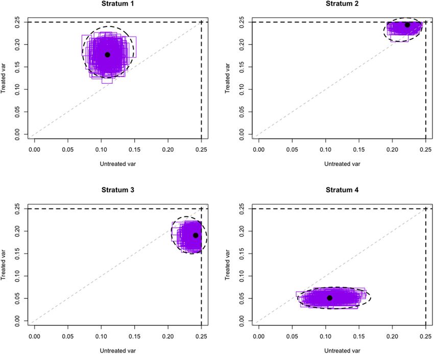
In Figure 1, we demonstrate this procedure on simulated data using Γ = 1.2 . We suppose there are four
strata, each containing 1,000 observational units. The strata differ in their treatment probabilities with 263,
421, 564, and 739 treated units in each stratum, respectively. The large black dot at the center of each cluster
represents the point estimate (σˆk2 (0) , σˆk2 (1)). In purple, we plot the rectangles corresponding to the extrema
computed in each of 200 bootstrap replicates drawn from the data. The dashed ellipsoids represent 90%
confidence sets. In the cases of strata 2 and 3, the ellipsoids extend beyond the upper bound of 0.25 in at
least one direction, so we intersect the ellipsoids with the hard boundary at 0.25. The resulting final
confidence sets, 1, 2 , 3, and 4 , are all convex.
The objective is convex in nrkt , nrkc and affine (and thus concave) in σk2 (1) , σk2 (0). Now, having obtained
convex constraints, we can invoke von Neumann’s minimax theorem [37] to switch the order of the mini-
mization and maximization. Hence, the solution to Problem (3) is equivalent to the solution of
⎛ ⎛ 1 1 ⎞ ⎛ 1 1 ⎞⎞
max2 min ∑wk ⎜σk2(1)⎜⎝ − ⎟ + σk2 (0)⎜ − ⎟⎟
2
σk (1), σk (0)nrkt , nrkc
k ⎝ nrkt n˜rkt ⎠ ⎝ nrkc n˜rkc ⎠⎠
subject to (σk2 (1) , σk2 (0)) ∈ (kΓ), k = 1, … , K
∑nrkt + nrkc = nr .
k
But the inner problem has an explicit solution, given by the expressions in (2). Plugging in these expres-
sions, we arrive at the simplified problem:
1⎛ ⎞2 ⎛ ⎛ σ 2 (1) σ 2 (0) ⎞⎞
max ⎜⎜∑ wk (σk (1) + σk (0))⎟⎟ − ⎜⎜∑wk ⎜ k + k ⎟⎟⎟
σk2 (1), σk2 (0) nr ⎝ k ⎠ ⎝ k ⎝ n˜rkt n˜rkc ⎠⎠ (7)
subject to (σk2 (1) , σk2 (0)) ∈ (kΓ), k = 1, … , K .
Problem (7) is concave. See Appendix C for a detailed proof. The solution is non-trivial, owing to the fact
that the problem is not DCP-compliant. Nonetheless, a simple projected gradient descent algorithm is
guaranteed to converge under very mild conditions given the curvature [38]. Similarly, under mild condi-
tions, the convergence rate can be shown to be linear (see e.g. ref. [39]), meaning that distance to the
optimum declines at a rate of O(1/m), where m is the number of steps taken by the algorithm. Hence, we can
efficiently solve this problem.Experiments informed by observational 155
Figure 1: Simulated example of confidence regions in four strata under Γ = 1.2.
5 Application to the data from the Women’s Health Initiative
5.1 Setting
To evaluate our methods in practice, we make use of data from the Women’s Health Initiative (WHI), a 1991
study of the effects of hormone therapy on postmenopausal women. The study included both an RCT and an
observational study. A total of 16,608 women were included in the trial, with half randomly selected to take
625 mg of estrogen and 2.5 mg of progestin, and the remainder receiving a placebo. A corresponding 53,054
women in the observational component of the WHI were deemed clinically comparable to women in the
trial. About a third of these women were using estrogen plus progestin, while the remaining women in the
observational study were not using hormone therapy [40].
We investigate the effect of the treatment on incidence of coronary heart disease. We split the data into
two non-overlapping subsets, which we term the “gold” and “silver” datasets. We estimate the probability
of treatment for observational units via fitted propensity scores. The data split is the same as the one used in
ref. [8]. Details on the construction of these data elements can be found in Section A.2, while further details
about the WHI can be found in Section A.1.
To choose our subgroups for stratification, we utilize the clinical expertise of researchers in the study’s
writing group. The trial protocol highlights age as an important subgroup variable to consider [41], while
subsequent work considered a patient’s history of cardiovascular disease [42]. To evaluate the impact of a156 Evan T. R. Rosenman and Art B. Owen
clinically irrelevant variable, we also consider langley scatter, a measure of solar irradiance at each
woman’s enrollment center, which is not plausibly related to baseline incidence or treatment effect. Langley
scatter exhibits no association with the outcome in the observational control population: a Pearson’s Chi-
squared test yields a p-value of 0.89. The analogous tests for age and history of cardiovascular disease have
p-values below 10−5.
The age variable has three levels, corresponding to whether a woman was in her 50s, 60s, or 70s. The
cardiovascular disease history variable is binary. The langley scatter variable has five levels, corresponding
to strata between 300 and 500 langleys of irradiance. We provide brief summaries of these variables in
Tables A.7–A.9 in Section A.3.
The RCT gold dataset is used to estimate “gold standard” stratum causal effects. We suppose that the
observational study is being used to assist the design of an experiment of size nr = 1,000 units. In all cases,
the default allocation is an equal allocation across strata and treatment statuses.
We face the additional challenge of choosing the appropriate value of Γ . The WHI provides a very rich
set of covariates, and our propensity model incorporates more than 50 variables spanning the demographic
and clinical domains (see details in Section A.2). Hence, we will run our algorithm at values of Γ = 1.0
(reflecting no residual confounding) as well as Γ = 1.1, 1.5, and 2.0 (reflecting a modest amount).
5.2 Detailed example: Γ = 1.5, fine stratification
We show one example in detail, in which we choose Γ = 1.5 and stratify on all three subgroup variables:
age, history of cardiovascular disease, and langley scatter. The cross-product of these variables yields 30
strata, which we suppose are weighted equally. We number these groups from 1 through 30.
In the top panel of Figure 2, we show a naïve RCT allocation based purely on the pilot estimates of the
stratum potential outcome variances from the observational study. In the bottom panel, we show the regret
minimizing allocations. Visually, it is clear that we have heavily shrunk the allocations toward an equally
allocated RCT, but there remain some strata where we recommend over- or under-sampling. Note, too, that
the shrinkage is not purely reflective of the magnitude of the pilot estimate, since the number of observa-
tional units from each stratum and treatment status also influences the width of our confidence region for
each of the pilot estimates.
To investigate the utility of our regret-minimizing allocations, we sample pseudo-experiments of 1,000
units from the RCT silver dataset 1,000 times with replacement. We do so under three designs: equal
allocation by strata; naïve allocation based on the pilot estimates; and the regret-minimizing allocations
under Γ = 1.5. We compute the average L2 loss when compared against the gold standard estimates derived
from the RCT gold dataset. Results are shown in Figure 3. Our method yields a modest reduction in average
loss (3.6%) relative to the naïve design. It also outperforms the equal design, though by a slimmer
margin (1.6%).
5.3 Performance over multiple conditions
We now simulate with all possible combinations of the stratification variables. For each choice of a stra-
tification, we sample 1,000 units from the RCT silver dataset with replacement, under equal allocation,
naïve allocation, and regret-minimizing allocation with Γ = 1.0, 1.1, 1.5, and 2.0. We then compute the L2
loss versus the “gold standard” estimates derived from the RCT gold dataset.
In Table 1, we summarize the loss of the regret-minimizing allocations relative to equal allocation. We
see immediately that the entries are all non-positive. This makes some intuitive sense: the objective in
Problem (3) can always be set to 0 by choosing nrkt = ñrkt and nrkc = ñrkc for all k ; hence, the algorithm is
designed to guarantee that we cannot do worse than allocating equally. By the same token, many of the
gains we see are modest, owing to the conservatism of the regret-minimizing approach. Notably, we seem toExperiments informed by observational 157 Figure 2: Allocation of units to strata under naïve allocation and regret-minimizing allocation. Figure 3: Average loss over 1,000 resamples of 1,000-unit experiments under equal allocation, naïve allocation, and regret- minimizing allocation designs.
158 Evan T. R. Rosenman and Art B. Owen
Table 1: L2 loss comparisons for regret-minimizing allocations relative to equal allocation
Subgroup Var(s) Equal alloc loss Loss relative to equal allocation
Γ = 1 (%) Γ = 1.1 (%) Γ = 1.5 (%) Γ = 2 (%)
Age 0.000517 −2.0 −1.9 −2.0 0.0
CVD 0.000498 −2.3 −2.0 −1.5 0.0
Langley 0.000841 0.0 0.0∗ 0.0∗ 0.0∗
Age, CVD 0.001541 −5.5 −5.6 −3.8 −2.3
Age, langley 0.003417 −1.6 −1.6 −0.7 −0.1
CVD, langley 0.002495 −1.7 −1.2 −0.8 −0.2
Age, CVD, langley 0.008395 −1.9 −2.1 −1.6 −0.7
∗For starred entries, the regret-minimizing allocation defaults to equal allocation.
achieve the greatest gains when we are stratifying only on clinically relevant variables and using a rela-
tively low value of Γ . We achieve a 5–6% risk reduction at low values of Γ in the fourth row of the table, in
which we stratify on the clinically relevant age and cardiovascular disease variables. On the other hand, the
algorithm quickly defaults to recommending equal allocation when variables are not clinically relevant. In
the third row, in which we stratify only on the irrelevant langley scatter variable, the starred entries
correspond to cases in which the regret-minimizing allocation is equal allocation.
In Table 2, we summarize the loss relative to naïve allocation. our method can underperform a naïve
allocation derived from the observational study pilot variance estimates. This can be seen most clearly in
the first row of the table, in which we stratify only on the age variable. However, there are two clear trends
in the results. First, when we stratify on a variable that turns out not to be clinically relevant, like langley
scatter, the naïve allocation is essentially recommending an allocation based on noise from the data; as a
result, our regret-minimizing allocations uniformly outperform naïve allocations. Second, the regret-mini-
mizing allocations tend to outperform the naïve allocations as the number of strata grows. We significantly
outperform naïve allocation in the final row, which corresponds to stratification on all three variables and a
total of 30 strata.
Recall that as Γ rises, the feasible set of Optimization Problem (3) grows larger. Hence, we expect the
allocation to be closer to the naïve allocation for smaller values of Γ , but to be regularized more toward the
default allocation for larger values of Γ . For large Γ , we would thus expect the loss to converge to the equal
allocation loss. This is precisely what we see in Table 1: for each possible stratification, the performance is
closest to that of the default allocation when Γ = 2 . However, in Table 2, we do not see the inverse pattern –
that is, performance is not uniformly closest to that of the naïve allocation when Γ = 1. This is because the
confidence set does not collapse to a single point at Γ = 1; rather, it incorporates the possibility of variance
but not bias in the pilot estimation. More broadly, we do not expect a monotone relationship between Γ and
the average loss. In many cases, the pilot estimates will be somewhat informative, but incorporate some
Table 2: L2 loss comparisons for regret-minimizing allocations relative to naïve allocation
Subgroup Var(s) Naïve alloc loss Loss relative to naïve allocation
Γ = 1 (%) Γ = 1.1 (%) Γ = 1.5 (%) Γ = 2 (%)
Age 0.000501 1.2 1.2 1.1 3.2
CVD 0.000488 −0.3 0.0 0.6 2.1
Langley 0.000852 −1.1 −1.3 −1.3 −1.3
Age, CVD 0.001484 −1.8 −1.9 −0.1 1.5
Age, langley 0.003393 −0.9 −0.9 0.0 0.6
CVD, langley 0.002481 −1.1 −0.7 −0.3 0.3
Age, CVD, langley 0.008574 −3.9 −4.1 −3.6 −2.8Experiments informed by observational 159
bias. Hence, we may see the lowest average loss at intermediate values of Γ , which encourage the algorithm
to extract some relevant information from the pilot data without relying too heavily on these estimates.
While these simulation results show modest performance gains, they are encouraging. A wise analyst
would be cautious about designing an RCT exclusively using observational study pilot estimates of poten-
tial outcome variances. Because such pilot estimates can have both bias and variance, relying too heavily
upon them might waste resources. Our framework allows data from the observational study to be incorpo-
rated into the RCT design while guarding against the possibility of underperforming a default allocation.
6 Extensions
We briefly discuss potential extensions of this work.
One natural consideration is the case of multiple treatment levels, rather than the binary setting of
treatment versus control. The machinery discussed in this manuscript naturally extends to the multilevel
case. If we suppose there are L treatment levels, then we instead optimize over sample sizes nrkℓ and stratum
potential outcome variances σk2 (ℓ) for ℓ ∈ {1, … , L} . The optimization problem becomes:
K L ⎛ 1 1 ⎞
min max ∑ wk ∑ σk2 (ℓ)⎜ − ⎟
{nrk ℓ}ℓ, k {σk2 (ℓ)}ℓ, k
k =1 ℓ=1
⎝ nrk ℓ n˜rk ℓ ⎠
subject to (σk2(1),…, σk2 (L)) ∈ (kΓ ), k = 1, …, K (8)
K L
∑∑nrk ℓ = nr .
k =1 ℓ=1
The curvature of Problem (8) is unchanged from that of Problem (3), so we can use the same von Neumann
trick to obtain a readily solvable concave maximization problem. The only remaining complexity is the
construction of the confidence sets (kΓ). The procedure described in Section 4.2 can be easily generalized to
the multilevel case, with the bounds derived from each bootstrap replicate now represented as an L-dimen-
sional box rather than a rectangle. The proof in Appendix B does not depend on the problem’s dimension-
ality, so we can again obtain asymptotic α -level validity for any confidence set drawn to include a 1 − α
proportion of the boxes. The method of drawing Löwner–John ellipsoids also generalizes to dimensions
greater than two, so we can use this exact procedure to obtain our confidence sets.
Another obvious extension is to the more general case of Yi ∈ . In keeping with the theme of IPW
estimation, we consider estimators of the form
⎛Z ⎞ ⎛ ⎛ Z i ⎞⎞
2
⎛ Z ⎞ ⎛Z ⎞
σˆk2 (1) = ∑ Yi2⎜ i ⎟ ∑⎜ i ⎟ − ⎜⎜ ∑Yi⎜ i ⎟ ∑ ⎜ ⎟⎟ ⎟
i∈ k
⎝ pi ⎠ ⎝ pi ⎠ ⎝ i ∈ k ⎝ pi ⎠
i∈ k
⎝ pi ⎠⎠
i∈ k
(9)
⎛ 1 − Zi ⎞ ⎛ ⎛ 1 − Z i ⎞⎞
2
⎛ 1 − Zi ⎞ ⎛ 1 − Zi ⎞
σˆk2 (0) = ∑Yi2⎜ ⎟ ∑⎜ ⎟ − ⎜⎜ ∑Yi ⎜ ⎟ ∑⎜ ⎟
⎟ ,
i∈ k
⎝ 1 − pi ⎠ ⎝ 1 − pi ⎠ ⎝ i ∈ k ⎝ 1 − pi ⎠
i∈ k
⎝ 1 − pi ⎠⎟⎠
i∈ k
where pi are the true treatment probabilities. Such estimators are asymptotically unbiased.
We suppose we estimate pi with fitted propensity scores, π̂i , defined as
1
πˆi = .
1 + e−gˆ (Xi)
T
We typically use logistic regression to estimate the propensity scores, such that gˆ (Xi ) = βˆ Xi .
We account for the possibility of Γ -level unmeasured confounding by allowing the true probability pi to
satisfy
⎧ 1 1 ⎫
pi ∈ ⎨ ≤ z i ≤ Γ⎬ .
⎩ 1 + zie−gˆ (Xi) Γ ⎭160 Evan T. R. Rosenman and Art B. Owen
We redefine the problem in terms of the vi = pi−1, an affine function of the zi . We define two vectors
vt = (vi )i : Zi = 1 and vc = (vi )i : Zi = 0, and analogously define vectors Yt = (Yi ) Zi = 1 and Yc = (Yi ) Zi = 0. Now, we can
express the equations in (9) as quadratic fractional programs, e.g.,
vtT Θt vt vcT Θc vc
σˆk2 (1) = , σˆk2 (0) = ,
vtT T vt vcT T vc
where
Θt = Yt2 T − YtYtT and Yc2 T − YcYcT .
We have few guarantees on the curvature of the problem: the numerators will be neither convex nor
concave in the ve terms, e ∈ {0, 1} , as long as the vectors , Yt , and Yt2 are linearly independent. The
denominators will be convex in the ve terms. This poses a major challenge. Quadratic fractional program-
ming problems can be solved efficiently in some special cases, but are, in general, NP-hard [43].
One avenue is to apply Dinkelbach’s method to transform the quadratic fractional problem to a series of
quadratic programming problems [44]. This would not immediately yield a solution because of the inde-
finite numerator, but it would potentially allow one to make use of considerable recent work on solution
methods in quadratic programming (see e.g. ref. [45]). This path represents a possible future extension of
this work.
Acknowledgments: We thank Mike Baiocchi, Guillaume Basse, and Luke Miratrix for their useful comments
and discussion.
Funding information: Evan Rosenman was supported by Google, and by the Department of Defense (DoD)
through the National Defense Science & Engineering Graduate Fellowship (NDSEG) Program. This work was
also supported by the NSF under grants DMS-1521145, DMS-1407397, and IIS-1837931.
Conflict of interest: The authors have no conflicts of interest to declare.
References
[1] Imbens GW, Rubin DB. Causal inference for statistics, social, and biomedical sciences: an introduction. New York:
Cambridge University Press; 2015.
[2] Hartman E, Grieve R, Ramsahai R, Sekhon JS. From SATE to PATT: Combining experimental with observational studies to
estimate population treatment effects. J R Stat Soc Ser A (Statistics in Society). 2015;10:1111.
[3] Writing Group for the Women’s Health Initiative Investigators. Risks and benefits of estrogen plus progestin in healthy
postmenopausal women: Principal results from the Women’s Health Initiative randomized controlled trial. J Am Med
Assoc. 2002;288(3):321–33.
[4] Campbell DT. Factors relevant to the validity of experiments in social settings. Psychol Bull. 1957;54(4):297.
[5] Zhao Q, Small DS, Bhattacharya BB. Sensitivity analysis for inverse probability weighting estimators via the percentile
bootstrap. J R Stat Soc Ser B (Statistical Methodology). 2019;81(4):735–61.
[6] Grant M, Boyd S, Ye Y. Disciplined convex programming. In: Global optimization. Boston, MA: Springer; 2006, p. 155–210.
[7] Bareinboim E, Pearl J. Causal inference and the data-fusion problem. Proc Natl Acad Sci. 2016;113(27):7345–52.
[8] Rosenman E, Owen AB, Baiocchi M, Banack H. Propensity score methods for merging observational and experimental
datasets. Technical report, 2018; arXiv:1804.07863.
[9] Athey S, Chetty R, Imbens GW, Kang H, The surrogate index: Combining short-term proxies to estimate long-term treat-
ment effects more rapidly and precisely. Technical report, National Bureau of Economic Research. 2019.
[10] Kallus N, Puli AM, Shalit U. Removing hidden confounding by experimental grounding. In: Advances in neural information
processing systems; 2018. p. 10888–97.
[11] Peysakhovich A, Lada A. Combining observational and experimental data to find heterogeneous treatment effects.
Technical report, 2016; arXiv:1611.02385.
[12] Page MJ, Shamseer L, Altman DG, Tetzlaff J, Sampson M, Tricco AC, et al. Epidemiology and reporting characteristics of
systematic reviews of biomedical research: a cross-sectional study. PLoS Medicine. 2016;13(5):e1002028.Experiments informed by observational 161
[13] Mueller M, D’Addario M, Egger M, Cevallos M, Dekkers O, Mugglin C, et al. Methods to systematically review and meta-
analyse observational studies: a systematic scoping review of recommendations. BMC Med Res Methodol. 2018;18(1):44.
[14] Thompson S, Ekelund U, Jebb S, Lindroos AK, Mander A, Sharp S, et al. A proposed method of bias adjustment for meta-
analyses of published observational studies. Int J Epidemiol. 2011;40(3):765–77.
[15] Prevost TC, Abrams KR, Jones DR. Hierarchical models in generalized synthesis of evidence: An example based on studies
of breast cancer screening. Stat Med. 2000;19(24):3359–76.
[16] Cooper GF, Yoo C. Causal discovery from a mixture of experimental and observational data. In: Proceedings of the
Fifteenth Conference on Uncertainty in Artificial Intelligence, UAI’99. San Francisco, CA, USA: Morgan Kaufmann
Publishers Inc; 1999. p. 116–25.
[17] Mooij JM, Magliacane S, Claassen T. Joint causal inference from multiple contexts. 2016; arXiv:http://arXiv.org/abs/
arXiv:1611.10351.
[18] Chambaz A, van der Laan MJ, Zheng W. Targeted covariate-adjusted response-adaptive lasso-based randomized con-
trolled trials. Modern adaptive randomized clinical trials: statistical, operational, and regulatory aspects; 2014.
p. 345–68.
[19] Hahn J, Hirano K, Karlan D. Adaptive experimental design using the propensity score. J Bus Econ Stat. 2011;29(1):96–108.
[20] Tabord-Meehan M. Stratification trees for adaptive randomization in randomized controlled trials. 2018; arXiv: http://
arXiv.org/abs/arXiv:1806.05127.
[21] Bai Y, Optimality of matched-pair designs in randomized controlled trials. 2019. Available at SSRN 3483834.
[22] Rubin DB. Estimating causal effects of treatments in randomized and nonrandomized studies. J Edu Psychol.
1974;66(5):688.
[23] Vander Weele TJ, Robins JM. Stochastic counterfactuals and stochastic sufficient causes. Statistica Sinica. 2012;22(1):379.
[24] A, Chin. Modern statistical approaches for randomized experiments under interference. PhD thesis. Stanford
University; 2019.
[25] Hill JL. Bayesian nonparametric modeling for causal inference. J Comput Graph Stat. 2011;20(1):217–40.
[26] Wager S, Athey S. Estimation and inference of heterogeneous treatment effects using random forests. J Am Stat Assoc.
2018;113(523):1228–42.
[27] Neyman J. On the two different aspects of the representative method: the method of stratified sampling and the method of
purposive selection. In: Breakthroughs in statistics. New York, NY: Springer; 1992. p. 123–50.
[28] Bell DE. Regret in decision making under uncertainty. Operations Research. 1982;30(5):961–81.
[29] Loomes G, Sugden R. Regret theory: An alternative theory of rational choice under uncertainty. Econom J.
1982;92(368):805–24.
[30] Diecidue E, Somasundaram J. Regret theory: A new foundation. J Econom Theory. 2017;172:88–119.
[31] Tan Z. A distributional approach for causal inference using propensity scores. J Am Stat Assoc. 2006;101(476):1619–37.
[32] Rosenbaum PR. Sensitivity analysis for certain permutation inferences in matched observational studies. Biometrika.
1987;74(1):13–26.
[33] Dorn J, Guo K. Sharp sensitivity analysis for inverse propensity weighting via quantile balancing. 2021; arXiv:http://arXiv.
org/abs/arXiv:2102.04543.
[34] Kallus N, Zhou A. Minimax-optimal policy learning under unobserved confounding. Manag Sci. 2021;67(5):2870–90.
[35] Hsu JY, Small DS. Calibrating sensitivity analyses to observed covariates in observational studies. Biometrics.
2013;69(4):803–11.
[36] Boyd S, Vandenberghe L. Convex Optimization. Cambridge, UK: Cambridge University Press; 2004.
[37] von Neumann J. On game theory. Proc Acad Sci. 1928;100(1):295–320.
[38] Iusem AN. On the convergence properties of the projected gradient method for convex optimization. Comput Appl Math.
2003;22(1):37–52.
[39] Saunders M. Notes on first-order methods for minimizing smooth functions. MS & E 318/CME 338: Large-Scale Numerical
Optimization Course Notes. 2018.
[40] Prentice RL, Langer R, Stefanick ML, Howard BV, Pettinger M, G, Anderson, et al. Combined postmenopausal hormone
therapy and cardiovascular disease: Toward resolving the discrepancy between observational studies and the Women’s
Health Initiative clinical trial. Am J Epidemiol. 2005;162(5):404–14.
[41] Writing Group for the Women’s Health Initiative Investigators. Design of the Women’s Health Initiative clinical trial and
observational study. Controlled Clinical Trials. 1998;19(1):61–109.
[42] Roehm E. A reappraisal of Women’s Health Initiative estrogen-alone trial: long-term outcomes in women 50–59 years of
age. Obstetrics and Gynecology International. 2015; 2015.
[43] Phillips AT. Quadratic fractional programming: Dinkelbach’s method. In: Encyclopedia of optimization. 2001; vol. 4.
[44] Dinkelbach W. On nonlinear fractional programming. Manag Sci. 1967;13(7):492–8.
[45] Park J, Boyd S. General heuristics for nonconvex quadratically constrained quadratic programming. Technical Report,
2017; arXiv:1703.07870.
[46] Hays J, Hunt JR, Hubbell FA, Anderson GL, Limacher M, Allen C, et al. The Women’s Health Initiative recruitment methods
and results. Ann Epidemiol. 2003;13(9):S18–S77.
[47] Rosenbaum P. Design of observational studies. Springer series in statistics. New York: Springer; 2009.162 Evan T. R. Rosenman and Art B. Owen
[48] Graziano AM, Raulin ML. Research methods: A process of inquiry. New York: HarperCollins College Publishers; 1993.
[49] Van der Vaart AW. Asymptotic statistics. Cambridge, UK: Cambridge University Press; vol. 3. 2000.
[50] Weyl H. The asymptotic distribution law for the eigenvalues of linear partial differential equations (with applications to the
theory of black body radiation). Math Ann. 1912;71(1):441–79.Experiments informed by observational 163
Appendix
A.1 Further details about the Women’s Health Initiative
We evaluate our estimators on data from the Women’s Health Initiative to estimate the effect of hormone
therapy on coronary heart disease (CHD). The Women’s Health Initiative is a study of postmenopausal
women in the United States, consisting of RCT and observational study components with 161,808 total
women enrolled [40]. Eligibility and recruitment data for the WHI can be found in the results of previous
studies [3,46]. Participants were women between 50 and 79 years old at baseline, who had a predicted
survival of at least 3 years and were unlikely to leave their current geographic area for 3 years.
Women with a uterus who met various safety, adherence, and retention criteria were eligible for a
combined hormone therapy trial. A total of 16,608 women were included in the trial, with 8,506 women
randomized to take 625 mg of estrogen and 2.5 mg of progestin, and the remainder receiving a placebo. A
corresponding 53,054 women in the observational component of the Women’s Health Initiative had an
intact uterus and were not using unopposed estrogen at baseline, thus rendering them clinically compar-
able [40]. About a third of these women were using estrogen plus progestin, while the remaining women in
the observational study were not using hormone therapy [40].
Participants received semiannual contacts and annual in-clinic visits for the collection of information
about outcomes. Disease events, including CHD, were first self-reported and later adjudicated by physi-
cians. We focus on outcomes during the initial phase of the study, which extended for an average of 8.16
years of follow-up in the RCT and 7.96 years in the observational study.
The overall rate of coronary heart disease in the trial was 3.7% in the treated group (314 cases among
8,472 women reporting) versus 3.3% (269 cases among 8,065 women reporting) for women not randomized
to estrogen and progestin. In the observational study, the corresponding rates were 1.6% among treated
women (706 out of 17,457 women reporting) and 3.1% among control women (1,108 out of 35,408 women
reporting). Our methodology compares means and not survival curves. In the initial follow-up period, death
rates were relatively low in both the observational study (6.4%) and the randomized trial (5.7%). Hence, we
do not correct for the possibility of these deaths censoring coronary heart disease events.
A.2 Propensity score construction, covariate balance, and gold standard effects
The Women’s Health Initiative researchers collected a rich set of covariates about the participants in the
study. For the purposes of computational speed, we narrow to a set of 684 variables, spanning demo-
graphics, medical history, diet, physical measurements, and psychosocial data collected at baseline.
The most meaningful measure of covariate imbalance can be found by looking at clinically relevant
factors. Prentice et al. [40] found that hormone therapy users in the observational study were more likely to
be Caucasian or Asian/Pacific Islander, less likely to be overweight, and more likely to have a college
degree. These imbalances strongly suggest that applying a naïve differencing estimate to the observational
data will yield an unfairly rosy view of the effect of hormone therapy on CHD.
To generate our estimators for this dataset, we need a propensity model e(x ) to map the observed
covariates to an estimated probability of receiving the treatment in the observational study. We used a
logistic regression to generate an expressive model while limiting overfit. A heuristic procedure was used
for careful construction of the propensity scores. Full details can be found in ref. [8].
Matching on the propensity score should reduce imbalances on clinically relevant covariates. We
provide a summary of these diagnostics, with additional details again available in ref. [8]. We use stan-
dardized differences to measure imbalance, as advocated by Rosenbaum [47].
We compute the standardized differences between treated and control on risk factors listed in ref. [40],
before and after adjusting for the propensity score by grouping the units into ten equal-width propensityYou can also read