Detailed reconstruction of trees from terrestrial laser scans for remote sensing and radiative transfer modelling applications
←
→
Page content transcription
If your browser does not render page correctly, please read the page content below
in silico Plants Vol. 3, No. 2, pp. 1–21
https://doi.org/10.1093/insilicoplants/diab026
Advance Access publication 27 August 2021
Special Issue: Functional-Structural Plant Models
Original Research

      Detailed reconstruction of trees from terrestrial
    laser scans for remote sensing and radiative transfer
                   modelling applications

                                                                                                                                                                                            Downloaded from https://academic.oup.com/insilicoplants/article/3/2/diab026/6358408 by guest on 29 October 2021
    Růžena Janoutová1,* , , Lucie Homolová1, Jan Novotný1, Barbora Navrátilová1,
                    Miroslav Pikl1 and Zbyněk Malenovský2
            1
              Department of Remote Sensing, Global Change Research Institute of the Czech Academy of Sciences, Bělidla 4a, 60300 Brno, Czech Republic
    2
        School of Geography, Planning, and Spatial Sciences, College of Sciences Engineering and Technology, University of Tasmania, Private Bag 76, TAS 7001
                                                                           Hobart, Australia
                                                *Corresponding author’s e-mail address: janoutova.r@czechglobe.cz

                                                         Guest Editor: Katrin Kahlen; Editor-in-Chief: Stephen P Long

    Citation: Janoutová R, Homolová L, Novotný J, Navrátilová B, Pikl M, Malenovský Z. 2021. Detailed reconstruction of trees from terrestrial laser scans for
                 remote sensing and radiative transfer modelling applications. In Silico Plants 2021: diab026; doi: 10.1093/insilicoplants/diab026

                                                                                     A B ST R A CT
                   This study presents a method for three-dimensional (3D) reconstruction of forest tree species that are, for
               instance, required for simulations of 3D canopies in radiative transfer modelling. We selected three forest species
               of different architecture: Norway spruce (Picea abies) and European beech (Fagus sylvatica), representatives of
               European production forests, and white peppermint (Eucalyptus pulchella), a common forest species of Tasmania.
               Each species has a specific crown structure and foliage distribution. Our algorithm for 3D model construction of
               a single tree is based on terrestrial laser scanning (TLS) and ancillary field measurements of leaf angle distribu-
               tion, percentage of current-year and older leaves, and other parameters that could not be derived from TLS data.
               The algorithm comprises four main steps: (i) segmentation of a TLS tree point cloud separating wooden parts
               from foliage, (ii) reconstruction of wooden parts (trunks and branches) from TLS data, (iii) biologically genuine
               distribution of foliage within the tree crown and (iv) separation of foliage into two age categories (for spruce trees
               only). The reconstructed 3D models of the tree species were used to build virtual forest scenes in the Discrete
               Anisotropic Radiative Transfer model and to simulate canopy optical signals, specifically: angularly anisotropic
               top-of-canopy reflectance (for retrieval of leaf biochemical compounds from nadir canopy reflectance signatures
               captured in airborne imaging spectroscopy data) and solar-induced chlorophyll fluorescence signal (for experi-
               mentally unfeasible sensitivity analyses).

               K E Y W O R D S : 3D tree reconstruction; influence of 3D forest structure; radiative transfer modelling; remote
               sensing; terrestrial laser scanning.

                         1. INTRODUCTION                                                              Based on the level of input details and type of outputs, RTMs can
Dynamic changes in forest ecosystem services, caused by climatic                                  be differentiated into simple one-dimensional (1D) models, follow-
changes, among other influences, are increasingly being assessed by                               ing a ‘big-leaf ’ concept that assumes homogeneous canopy in hori-
remote sensing (RS) methods (Correa-Díaz et al. 2019; Zellweger                                   zontal dimensions, and more-detailed 3D models, capturing canopy
et al. 2019) that allow monitoring large areas within relatively short                            heterogeneity in all three spatial dimensions (Widlowski et al. 2015;
time periods. Radiative transfer models (RTMs) providing a physical                               Malenovský et al. 2019). The models’ simulations are used in a
link between leaf and canopy biochemical and structural properties                                wide range of applications, including sensor data simulations, inter-
and canopy reflectance are tools frequently used for RS interpretation                            pretation of RS images and sensitivity studies of RS optical sig-
(van der Tol et al. 2019; Verrelst et al. 2019).                                                  nals (Verhoef 1998; Ligot et al. 2014). Detailed inputs and precise

© The Author(s) 2021. Published by Oxford University Press on behalf of the Annals of Botany Company.
This is an Open Access article distributed under the terms of the Creative Commons Attribution License (https://creativecommons.org/licenses/by/4.0/), which permits unrestricted
                                                                                                                                                                                    •   1
reuse, distribution, and reproduction in any medium, provided the original work is properly cited.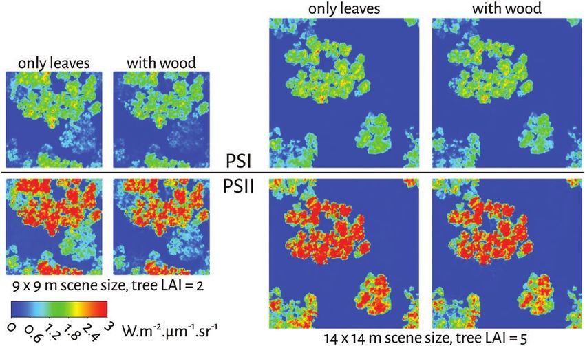
2   •   Janoutová et al.

radiative transfer (RT) computations are essential, as exemplified in      are often hollow and not tightly connected, thus allowing simulated
sensitivity studies, for example, where all aspects of a given object of   photons or light rays to enter the primitives, and that subsequently
interest must be included ( Janoutová et al. 2019; van der Tol et al.      leads to uncertainties in RT modelling results. Additionally, the spa-
2019; Lukeš et al. 2020; Malenovský et al. 2021), or in RS retriev-        tial and angular distribution of the foliage, which is crucial for simu-
als of vegetation biophysical parameters, where a large number of          lating light scattering processes, is not addressed by QSM, as it is less
RT-simulated scenes capturing the natural variability of an observed       important for biomass estimations. An alternative option is to use
phenomenon is required (Malenovský et al. 2013; Verrelst et al.            functional–structural plant models (FSPMs), which are designed
2019). In this study, we provide examples of both applications, spe-       to be very accurate in the sense of how they structurally represent
cifically: (i) retrieval of quantitative biophysical parameters from RS    the tree (Woodhouse and Hoekman 2000; Disney et al. 2006). The
hyperspectral observations of Norway spruce forests (Appendix A)           greatest disadvantage of this approach is that it requires many input
and (ii) RT-simulated impact of canopy woody components on emis-           parameters. A great many physiological parameters for a given spe-

                                                                                                                                                       Downloaded from https://academic.oup.com/insilicoplants/article/3/2/diab026/6358408 by guest on 29 October 2021
sion and escape of solar-induced chlorophyll fluorescence (SIF) of a       cies, as well as environmental growth conditions during the species’
white peppermint forest stand (Appendix B). In both cases, optimiz-        whole lifespan, are needed for constructing FSPMs (Leersnijder
ing 3D complexity of simulated forest stands was crucial to achieving      1992; Woodhouse and Hoekman 2000; Ong et al. 2014; Sievänen
desirable accuracy while keeping a reasonable simulation computa-          et al. 2014; Fabrika et al. 2019). Once an FSPM is properly param-
tional time of all the thousands of input combinations. We used the        eterized, however, it is possible to reconstruct the tree at any age
Discrete Anisotropic Radiative Transfer (DART) model (Gastellu-            and in any conditions, and that is in contrast to 3D reconstruction
Etchegorry et al. 1996, 2015, 2017) for its capability to import and       derived from TLS data, which corresponds to a single data acquisi-
work with detailed 3D objects of trees (Gastellu-Etchegorry et al.         tion time point (Woodhouse and Hoekman 2000).
2015; Liu et al. 2019b; Malenovský et al. 2021) and to simulate opti-           The approach described in this study offers universal recon-
cal signals of a large number of scenes within an acceptable time          struction of trees based on TLS data. It was applied to data sets that
frame (Homolová et al. 2016; Abdelmoula et al. 2018).                      differ in terms of laser scanning technical specifications and acqui-
    The tree species used in this study are (i) Norway spruce (Picea       sition conditions, given by both locally available instrumentation
abies), a representative of European mountain production forests; (ii)     and site-specific local situations. Inasmuch as the first version of our
white peppermint (Eucalyptus pulchella), a common forest species           3D tree reconstruction algorithm already had been developed and
endemic to Tasmania (Australia); and (iii) European beech (Fagus           customized for conifer Norway spruce (Sloup 2013; Janoutová et al.
sylvatica), a representative of European temperate production forest.      2019), the goal of this study was to extend and test the algorithm
Norway spruce is an evergreen coniferous species with a complex            on broadleaf tree species (i.e. European beech and white pepper-
and, from a modelling point of view, challenging crown structure, due      mint). Species-specific TLS data collected by different scientists
to its needle-shaped leaves forming shoots of several age categories       on two continents gave us an opportunity to assess robustness of
(between five and seven shoot-age categories can be present within a       the approach and to test how it copes not only with different tree
single tree crown). The occurrence of shoot ages as well as the actual     architectures but also with various scanning conditions, instrument
leaf/shoot angle distribution (LAD) were obtained from destructive         settings and data processing. Further we used forest reflectance simu-
field measurements (Barták 1992; Barták et al. 1993). White pepper-        lations in the DART model to demonstrate differences in parameteri-
mint is an evergreen broadleaf species having leaves of mainly two age     zation of tree 3D architecture, spanning from the most complex 3D
categories, which are highly clumped and predominantly distributed         tree representations to simple trees formed by geometric primitives
according to an erectophile LAD (Wiltshire and Potts 2007; Pisek and       and turbid leaf media.
Adamson 2020). European beech is a deciduous broadleaf species,
having simple-shaped leaves of the same age distributed evenly accord-                2. M AT E R I A L S A N D M ET H O D S
ing to a planophile LAD (Chianucci et al. 2018), as do the majority of                               2.1 Study sites
European broadleaf tree species.                                           Basic characterization of all study sites where input data were col-
    Three-dimensional reconstruction of a virtual tree can be per-         lected is shown in Table 1. All listed information is relevant to the
formed in several ways, depending upon its application purpose. One        date of data acquisition, which differs from site to site. Only three
of the ways most frequently used is reconstruction from terrestrial        study sites were used for collecting TLS data: Černá hora in the
laser scanning (TLS) measurements through so-called quantita-              Czech Republic for Norway spruce; Hobart in Tasmania, Australia
tive structure models (QSMs; Raumonen et al. 2013; Calders et al.          for white peppermint; and Těšínské Beskydy in the Czech Republic
2015). This approach has been used for above-ground biomass esti-          for European beech. Two remaining sites, Bílý Kříž and Štítná, both
mation (Calders et al. 2015; Disney et al. 2018) and also for forest       in the Czech Republic, were used to collect supporting data, such as
inventory purposes (Raumonen et al. 2015; Bienert et al. 2018). To         leaf optical, biochemical and other structural properties. Each of the
meet the application requirements, QSMs are optimized to compute           latter is a part of a permanent experimental research network created
the volume of the wooden biomass, where geometrical reconstruc-            around an eddy-covariance flux measuring tower. Their permanency
tion of wooden parts is a side product. Consequently, trees are rep-       resulted in collecting a large amount of continuous measurements
resented by a set of geometrical primitives, such as cylinders and         during several multi-scale field campaigns, which serve as the source
cones (Raumonen et al. 2013; Markku et al. 2015), which is insuf-          of data for our study. The geographical locations of the study sites are
ficient for RS applications simulating radiant fluxes. The primitives      depicted in Fig. 1.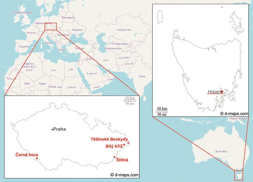
Table 1. Basic characteristics of study sites used in this study. The table shows information relevant at the time of input data acquisition.
Characteristics                      Černá hora                  Hobart                        Těšínské Beskydy             Bílý Kříž 1                     Bílý Kříž                           Štítná 1
Location                             Czech Republic              Australia                     Czech Republic               Czech Republic                  Czech Republic                      Czech Republic
Latitude                             48°58′22″ N                 42°54′57″ S                   49°35′42″ N                  49°30′ N                        49°30′17″ N                         49°2′14″ N
Longitude                            13°32′54″ E                 147°17′50″ E                  18°47′31″ E                  18°32′ E                        18°32′28″ E                         17°58′5″ E
Elevation [m a.s.l.]                 1250–1300                   330                           500–600                      850–900                         870                                 520–620
Forest composition                   Norway spruce               White peppermint              Mixed forest2                Norway spruce                   Norway spruce                       European beech
Forest age [years]3                  100                         Varying age                   80–100                       40                              35                                  109
Mean forest height [m]               25                          4.7–16.2                      32–36                        17                              13                                  31
Stand density [trees·ha−1]           800                         Not measured                  260–300                      1230                            2004                                282
Slope orientation                    SSE                         Flat                          NW, W                        S                               SW                                  SW, W, NW
Slope gradient                       7°                          Flat                          15–30°                       12.5°                           Slight                              10°
Data acquisition                     2009 (TLS)4                 2017/2018 (TLS)               2019 (TLS)                   2016 (biochemistry)             1990 (leaf distribution)            2011 (leaves)
                                                                                                                                                                                                2013 (biochemistry)
References                           –                           Wallace et al. (2016)         Grigorieva et al.            Urban et al. (2012);            Barták (1992);                      Darenova et al. (2016);
                                                                                                 (2020); IFER5                Darenova et al.                 Barták et al. (1993)                Marková et al.
                                                                                                                              (2016); Homolová                                                    (2017); McGloin
                                                                                                                              et al. (2017);                                                      et al. (2018)
                                                                                                                              Krupková et al.
                                                                                                                              (2017); McGloin
                                                                                                                              et al. (2018)
1
  This site facilitates long-term research of tree ecophysiology and carbon fluxes and is part of the national Czech Carbon Observation System (CzeCOS). Bílý Kříž is a class 2 station of the international Integrated Carbon
Observation System (ICOS) research network.
2
 Studied forest stands are dominated by European beech (Fagus sylvatica) and Norway spruce (Picea abies) with interspersed sycamore maple (Acer pseudoplatanus), northern red oak (Quercus rubra), European ash (Fraxinus
excelsior) and silver birch (Betula pendula).
3
 At the time of data acquisition.
4
 The Černá hora site had been severely damaged by multiple bark beetle outbreaks about 1–2 years prior to the TLS data acquisition in 2009. This pest outbreak allowed acquisition of high-density laser scans of surviving
individuals that were previously growing inside a close canopy.
5
 Data were provided by IFER–Institute of Forest Ecosystem Research Ltd. and IFER–Monitoring and Mapping Solutions, Ltd.
                                                                                                                                                                                                                                 Detailed reconstruction from TLS for RS apps
                                                                                                                                                                                                                                 •
                                                                                                                                                                                                                                 3

                                  Downloaded from https://academic.oup.com/insilicoplants/article/3/2/diab026/6358408 by guest on 29 October 2021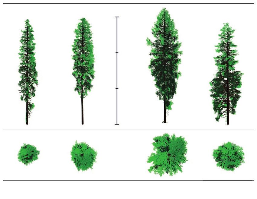
4   •   Janoutová et al.

                                                                                                                                                          Downloaded from https://academic.oup.com/insilicoplants/article/3/2/diab026/6358408 by guest on 29 October 2021
Figure 1. Locations of study sites (labelled in red) providing inputs for this study.

           2.2 TLS and 3D tree reconstruction                                    The white peppermint TLS points of each tree were semi-automat-
TLS scans for each tree species were obtained during three independ-         ically separated into two groups: (i) points of trunks and branches and
ent field campaigns. Technical characteristics of each TLS acquisition       (ii) points representing green foliage. The separation was done, as in
are summarized in Table 2. The reconstruction algorithm consists of          the previous case of Norway spruce, by thresholding scans of every
the following four steps (illustrated in Fig. 2): (i) segmentation of a      scanning position separately in CloudCompare software version 2.9
TLS tree point cloud separating wooden parts from foliage, (ii) recon-       (CloudCompare 2017). After the separation of wooden parts and
struction of trunk and branches (Sloup 2013) based on the point cloud        foliage points, the scans of all measuring positions were merged and
of wooden parts, (iii) distribution of foliage within the tree crown         manually cleaned for obvious outliers (Malenovský et al. 2021).
using the points of foliage cloud as attractors and (iv) generation of a          We were, unfortunately, unable to apply the thresholding approach
3D representation by merging the reconstructed wooden and foliage            for separating woody and foliage parts in the case of European beech,
objects ( Janoutová et al. 2019).                                            because the TLS intensity values did not have the required bimodal
    The first step of our tree reconstruction method (i.e. segmentation      distribution. The separation was, therefore, done manually. Since it is
of TLS point clouds) was different for each tree species due to techni-      a time consuming process when usual 2D view methods (e.g. editing
cal differences in laser scanners and their settings.                        in CloudCompare) are used, we improved the efficiency of the manual
    The PolyWorks IMSurvey module was used to filter out individual          editing by employing the LidarViewer software (Kreylos et al. 2008)
Norway spruce tree point clouds and to separate wooden and foliage           built on top of the Virtual Reality User Interface (Vrui) toolkit (Kreylos
points based on intensity of the reflected laser signals. Considering that   2008). The main advantage of using the 3D virtual reality approach is
green foliage reflects about 10 % and wooden parts as much as 50 %           its capability of direct 3D interactions with points in the entire point
of the laser signal at 1.5 µm, we determined the intensity thresholds        cloud (i.e. whole scanned plot) at adjustable spatial scales. This allows
between foliage and wooden parts per scan from first and last returns        for effective and accurate distinction, selection and export of individ-
of two opposite scanning positions separately ( Janoutová et al. 2019).      ual points representing trees’ wooden and foliage parts. Using the 3D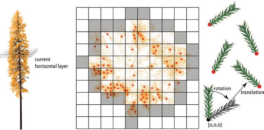
Detailed reconstruction from TLS for RS apps      •   5

Table 2. Overview of technical specifications of TLS used for tree scanning and their settings.
TLS parameter                Černá hora                               Hobart                                 Těšínské Beskydy
Scanner                      OPTECH Ilris-36D                         Trimble TX8                          Riegl VZ-400
Manufacturer                 Teledyne Optech, Vaughan, ON,            Trimble, Sunnyvale, CA, USA          RIEGL Laser Measurement Systems,
                                Canada                                                                        Horn, Austria
Wavelength [µm]              1.5                                       1.5                                 1.5
Maximum field-of-view        40° × 40°                                 360° × 317°                         360° (azimuth)
                                                                                                           100° (30°–130°; zenith)
Data acquisition             2009                                      2017/2018                           2019
Scanning design              • Each tree was scanned from two         • Multi-scans from several (4–10)  • Multi-scans from the centre and

                                                                                                                                                        Downloaded from https://academic.oup.com/insilicoplants/article/3/2/diab026/6358408 by guest on 29 October 2021
                                opposing positions, recording the         positions.                          four quadratic directions of the
                                first and the last echo return with • Point spacing of 11.3 mm at            plot.
                                the point sampling distance of            distance of 30 m.                • One upright and one tilted scan at
                                2 cm.                                                                         every position to cover the whole
                                                                                                              hemisphere around the scanner.
                                                                                                           • Several beech trees were separated
                                                                                                              from complex TLS scenes.
Processing                   • Point clouds of first and last returns • Point clouds of first and last   • Point clouds of multiple returns of
                                of each individual tree were              returns of each individual tree     each individual tree were aligned
                                aligned and co-registered using           were aligned and co-registered      and co-registered and processed
                                the PolyWorks IMAlign module              using a scan-to-scan matching in    in RiScan Pro (RIEGL Laser
                                (InnovMetric Software Inc.,               Trimble Realworks 10.1. (Trimble, Measurement Systems, Horn,
                                Quebec City, QC, Canada).                 Sunnyvale, CA, USA).                Austria).

virtual reality technique significantly shortened the time required for      is available in the study of Janoutová et al. (2019). Again, the algo-
the manual separation to approximately 1 day per tree, compared to at        rithm for distribution of 3D foliage elements was primarily designed
least 7 days when using a conventional 2D viewing method.                    for Norway spruce and here it was customized to suit the two broad-
     The second step (i.e. reconstruction of trunk and branches)             leaf species. The modification consisted of two adjustments. First, leaf
uses an automated algorithm based on the method of Verroust and              angular orientation was based on predefined LAD functions, because
Lazarus (1999) and can be summarized in three consecutive parts:             direct measurements of individual leaves’ orientation was not avail-
(i) component identification, (ii) component analysis and (iii) con-         able. Instead, we defined the angular orientation according to indirect
necting components. Detailed description of all parts in the wood            optical measurements as erectophile for eucalyptus family species
reconstruction algorithm is in the study of Sloup (2013). Although           (Danson 1998; Pisek and Adamson 2020) and planophile for beech
this algorithm was originally designed for Norway spruce, here it was        trees (Chianucci et al. 2018; Liu et al. 2019a). This modification was
tested on other tree species. In the end, its application to broadleaf       implemented by loading the LAD probability function from an exter-
tree species required only minor modification of input parameters.           nal file, which allows the algorithm to switch to another LAD function
Some reconstructed parts were slightly deformed, e.g. too-thick or           whenever needed. Second, the separation of foliage objects into two
too-thin trunk and branches, but these insufficiencies were corrected        age classes was not applied. Even though white peppermint is an ever-
by optimizing the input parameter called distanceLimit (section 4.2          green species and its trees retain more than one generation of leaves,
in Sloup 2013), which prevented the algorithm from interconnecting           this feature was disabled due to a lack of data. It can be enabled once
points of different branches. The algorithm failed only in a special         information about the spatial distribution of current and older leaves
case, when the tree trunk was split into two equally thick parts at the      becomes available.
very bottom. The wooden point cloud had to be split in two logical               The needle shoot representation used in this study was created
parts by an operator and the reconstruction was then run for each            for the RAdiation transfer Model Intercomparison exercise (RAMI
part separately.                                                             IV) (Table 3; Widlowski et al. 2015), then adapted and simplified for
     The third step of our algorithm (i.e. distribution of 3D foliage ele-   use in RT modelling in collaboration with DART scientists. Three-
ments − leaf or needle shoots) is conducted in the following three           dimensional representation of a white peppermint leaf was created
parts: (i) calculation of foliage elements’ positions and their angular      based on an average shape and size of actual leaves depicted in the
orientation, (ii) division of foliage into age classes (only if required,    guide to the eucalypts of Tasmania by Wiltshire and Potts (2007).
i.e. for evergreen tree species) and (iii) positioning of foliage elements   Creation of a 3D object representing a European beech leaf was car-
and their angular orientations (Fig. 3). Detailed description of all parts   ried out based on field measurements acquired at the Štítná study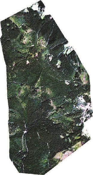
6   •   Janoutová et al.

                                                                                                                                             Downloaded from https://academic.oup.com/insilicoplants/article/3/2/diab026/6358408 by guest on 29 October 2021
Figure 2. Methodological steps of the 3D reconstruction approach, illustrated by the case of a spruce (from left to right): (i) TLS
tree point cloud segmentation (A), (ii) reconstruction of wooden parts [trunk and branches, (B)], (iii) distribution of foliage
within the tree crown [TLS points acting as attractors, (C)], and (iv) generation of a 3D representation (D).

Figure 3. Illustration of the algorithm for distribution of Norway spruce shoot representations within a tree crown in three
steps: (i) calculation of shoots’ positions (red dots) and rotations, (ii) division of shoots into two age classes (current-year and
older) and (iii) translation of each shoot from its original coordinates (the black dot) into predefined positions (red dots) and
angular orientations. The grey voxels correspond to the convex hull of a tree crown in the visualized horizontal layer and serve for
identification of the current-year shoots’ positions.

site in 2011. Several beech leaves were scanned using a flatbed scan-   Inkscape version 0.92 (Inkscape Project 2017), simplified and then
ner at 600 dpi resolution and their mean areas were calculated from     converted into a 3D object in Blender version 2.79 (Blender Online
the scans. In both cases, the digital representation was created in     Community 2017) (Table 3).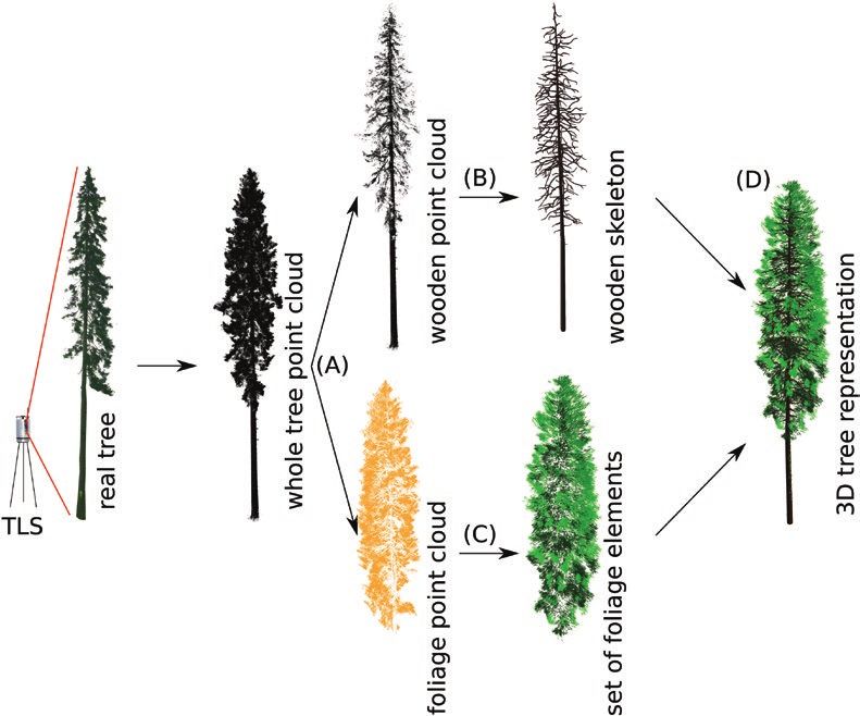
Detailed reconstruction from TLS for RS apps        •   7

Table 3. Foliage objects used to generate 3D tree representations. The leaf area and number of facets in each foliage object were
exported from the Blender software (Blender Online Community 2017).
Tree type                                                Norway spruce                                 White peppermint                        European beech

Detailed leaf/shoot
                                                           1

                                                                                                                                                                        Downloaded from https://academic.oup.com/insilicoplants/article/3/2/diab026/6358408 by guest on 29 October 2021
Simplified leaf/shoot

Leaf area [cm2]                                                 38.022                                      2.73                                    12.21
Number of facets (detailed/simplified)                         8243/16                                      33/2                                    202/6
1
  According to Widlowski et al. (2015).
2
 Outer area of needles only (i.e. half of the Blender generated value) and without the central twig.
3
 Sum of all twig and needle facets.

   Within the last step, the reconstructed wooden and foliage objects                      out of geometrical primitives (facets) representing foliage and wooden
were merged together to form the final 3D tree representation.                             parts. The DART model also allows users to combine both approaches.
                                                                                           Technical details on different tree parameterizations offered in DART
    2.3 Comparison of different tree parameterizations                                     are summarized in the DART User’s Manual (Gastellu-Etchegorry
There are several levels of a tree abstraction applicable in RT simula-                    2021) or in Janoutová et al. (2019).
tions, starting from a highly detailed geometrically explicit tree up to                        To demonstrate the impact of differently detailed 3D tree abstrac-
a simple generic tree with a crown represented as a turbid media. We                       tions on the DART-simulated top-of-canopy reflectance, we created
simulated forest reflectance of three different tree representations in the                for each tree species a set of three forest scenes ranging from the most
DART model (Gastellu-Etchegorry et al. 1996, 2015, 2017) to demon-                         complex to the most simplest 3D representation. Details of tree struc-
strate the impact of tree 3D structure details on the canopy reflectance.                  tural parameterizations were maintained and generalized as follows:
In the simplest parameterization tree crown shapes are approximated                        (i) 3D detailed tree representations were retained as geometrical facets
as regular 3D geometric shapes built out of voxels filled with a turbid                    (i.e. a ‘3D detailed’ scenario); (ii) 3D detailed tree representations had
medium. The turbid medium voxels are filled with an infinite number                        foliage transformed into turbid medium (i.e. a ‘turbid’ scenario); and
of infinitely small leaves characterized by predefined leaf optical and                    (iii) predefined simple 3D tree crown shapes, in our cases ellipsoidal,
structural properties. Structural properties are defined primarily by                      were filled with a turbid medium and contained simple straight trunks
leaf area index (LAI) and LAD, both specified either per tree or per                       without branches (i.e. a ‘simple’ scenario).
canopy of the entire simulated scene. Other controlling parameters are                          In some cases, the 3D tree representations had to be spatially
distribution of empty voxels (i.e. canopy air gaps) and leaf volume den-                   scaled, because the TLS data were acquired for trees of different
sity inside a voxel, both mimicking variable foliage clumping, that can                    height than the site for which RT simulations were performed. This
be specified either per crown or according to crown vertical level. In                     was done by scaling dimensions of the input TLS point clouds, in the
the most detailed and precise tree parameterization the 3D tree repre-                     case of Norway spruce trees by scaling factor 0.6 and in the case of
sentations are built as described in the previous sections, i.e. composed                  European beech by scaling factor 0.7 (white peppermint trees were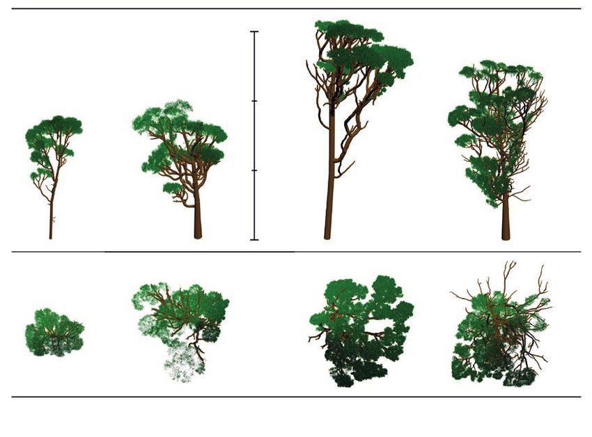
8   •     Janoutová et al.

kept unscaled). The scaling was employed to keep the scene dimen-         in the PROSPECT-D leaf RTM (Féret et al. 2017) according to input
sions fixed to 10 × 10 m across the species and to achieve comparable     parameters are listed in Table 5. The simulated directional-hemispher-
canopy cover (CC, 80 %) while using at least four individual trees in     ical leaf reflectance and transmittance are shown in Fig. 4 (left). The
the scene (Table 4).                                                      optical properties for woody twigs, stem bark and ground (Fig. 4,
    All other input parameters (e.g. optical properties, CC and scene     right) were measured during a field campaign in 2016 at the study site
LAI) were unified to ensure that the results are influenced only by the   Bílý Kříž (Table 1; Homolová et al. 2017).
tree structural parametrization. The DART scene input parameters are
summarized in Table 4. The foliage optical properties were simulated                 3. R E S U LTS A N D D I S C U S S I O N
                                                                                           3.1 3D tree representations
                                                                          The results reported in Table 6 confirm the successful extension and
Table 4. DART scene parameters used to simulate forest
                                                                          application of the algorithm developed in Janoutová et al. (2019) to

                                                                                                                                                        Downloaded from https://academic.oup.com/insilicoplants/article/3/2/diab026/6358408 by guest on 29 October 2021
reflectance of three species: Norway spruce, white peppermint
                                                                          the other two tested broadleaf tree species. Four individuals per species
and European beech.
                                                                          were successfully reconstructed despite that white peppermint (Fig.
Species                      Norway            White        European      6) and European beech (Fig. 7) occupy contrasting habitats and have
                             spruce          peppermint      beech        very different tree crown architectures compared to Norway spruce.
                                                                          Additionally, the TLS input data of each species were acquired using
Scene size [m × m]           10 × 10           10 × 10        10 × 10
                                                                          an instrument of different technical design, specifications and setup,
Cell size [m]                  0.2               0.2            0.2
                                                                          and that data also were processed differently. This suggests that our
CC [%]                         80                80             80
                                                                          reconstruction algorithm is sufficiently robust to use TLS data that dif-
Scene LAI [m2·m−2]              8                 8              8
                                                                          fer in terms of acquisition parameters and processing levels. It also can
Number of trees in scene       10                 5              4
                                                                          handle significant variation in trunk and branch shapes, as well as in the
                                                                          foliage spatial and angular distribution that appears among, but also
                                                                          within, the biological species, as documented in Figs 5–7 and Table 6.
Table 5. Input parameters used in PROSPECT-D leaf                              The main advantage of the algorithm is its ability to reconstruct an
RTM to simulate leaf optical properties (i.e. reflectance and             extensive variety of trees across and within given species from a rela-
transmittance).                                                           tively small amount of input data. The largest structural variability orig-
                                                                          inates from structural differences between tree species, spanning in this
Parameter                                             Leaves/needles      study from regularly organized spruce crowns, with branches growing
Chlorophyll content [µg·cm ] −2
                                                            43.15         in whorls carrying symmetrical needle shoots; to irregularly distrib-
Carotenoid content [µg·cm−2]                                 9.18         uted large and dense clumps of broad leaves, characteristic for white
Dry matter content [g·cm−2]                                  0.017        peppermint; and to smaller, sparse leaf clumps of European beech
Water content [g·cm−2]                                       0.021        organized more regularly in the vertical dimension. Nonetheless, addi-
Structural parameter [−]                                     1.9          tional within-species variability originates from ecological interactions
Fraction of brown pigments [−]                               0            and environmental disturbances, such as competition among neigh-
Anthocyanin content [µg·cm−2]                                0            bouring trees for resources (e.g. for photosynthetically active radia-
                                                                          tion, water and nutrients) causing variation in tree height (dominant

Figure 4. Leaf reflectance and transmittance spectra generated for DART simulations by PROSPECT-D (left), and measured
directional-hemispherical reflectance of shoot twigs, stem bark and ground cover (right). These optical properties were used in all
scenarios.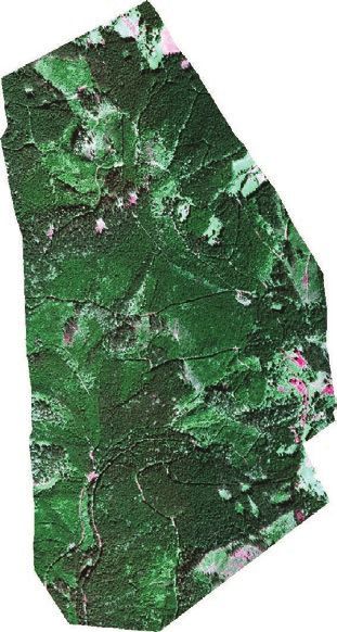
Detailed reconstruction from TLS for RS apps   •   9

Table 6. Characteristics of 3D tree representations produced for the three investigated tree species. The characteristics relate to
trees with detailed forms of shoots or leaves, as listed in Table 3. Differences in tree LAI are due to different requirements of target
applications using the 3D tree representations.
                                                                         Parameter
                       Tree height [m]   Crown length [m]   Crown diameter       Crown diameter           Number of       Number of leaf
                                                             in x-axis [m]        in y-axis [m]           wood facets        facets
Norway spruce (LAI 12)
  S. tree 1             15.0                  14.5               2.88                  2.48                 112 448        11 750 240
  S. tree 2             15.3                  10.5               3.03                  3.01                 106 112        15 757 352
  S. tree 3             16.4                  14.2               4.13                  3.93                 186 432        28 014 352

                                                                                                                                            Downloaded from https://academic.oup.com/insilicoplants/article/3/2/diab026/6358408 by guest on 29 October 2021
  S. tree 4             14.8                  14.6               4.56                  4.27                 197 760        28 594 448
White peppermint (LAI 5)
  P. tree 1              9.44                  4.86              4.09                  3.60                  87 122         4 203 672
  P. tree 2             10.47                  7.20              6.76                  6.57                 147 374        10 611 645
  P. tree 3             15.97                  5.72              8.15                  7.80                 124 098        17 943 090
  P. tree 4             13.19                 10.56              6.97                  8.60                 281 622         6 957 225
European beech (LAI 12)
  B. tree 1             21.2                  18.32              7.36                  8.30                  50 820        21 756 006
  B. tree 2             27.2                  16.60             11.12                  8.21                 100 322        20 288 678
  B. tree 3             22.3                  13.66              5.86                  7.88                 132 330        20 057 186
  B. tree 4             16.8                  15.72              5.70                  6.22                  37 686        23 561 886

S, Spruce; P, Peppermint; B, Beech.

Figure 5. Four Norway spruce tree 3D representations (A-D) reconstructed from TLS data point clouds acquired with an
OPTECH Ilris-36D instrument. Colour rendering indicates wooden parts in dark brown, current-year needle shoots in light
green and older needle shoots in dark green ( Janoutová et al. 2019).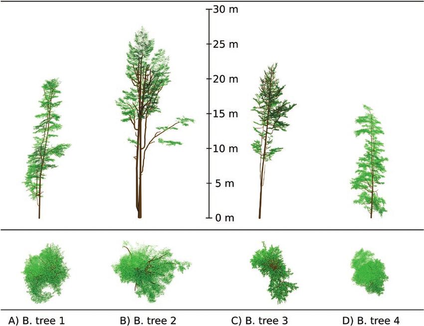
10 •    Janoutová et al.

                                                                                                                             Downloaded from https://academic.oup.com/insilicoplants/article/3/2/diab026/6358408 by guest on 29 October 2021
Figure 6. Four white peppermint tree 3D representations (A-D) reconstructed from TLS data point clouds acquired with a
Trimble TX8 instrument. Colour rendering indicates wooden parts in brown and leaves in green.

Figure 7. Four European beech tree 3D representations (A-D) reconstructed from TLS data point clouds acquired with a Riegl
VZ-400 instrument. Colour rendering indicates wooden parts in brown and leaves in green.
Detailed reconstruction from TLS for RS apps • 11
vs suppressed trees) or strong wind gusts causing irregularities in tree segmentation of leaves and wooden tree parts, but neither of our TLS
crowns (e.g. missing and broken branches). The algorithm seems capa- data has sufficient point density to test the method. However, it will be
ble of capturing all these naturally occurring biotic and abiotic impacts. desirable to test that approach and possibly to implement it in our future
The only required algorithm inputs are the following: TLS point processing once suitable TLS data are acquired.
clouds, information about foliage distribution (e.g. LAD function) and Finally, creation of the 3D foliage element object is not a lim-
a representative 3D object of crown foliage elements. Generally speak- iting factor. It is straightforward and, especially for broadleaf spe-
ing, the accuracy achieved is greater for denser and more precise TLS cies, easy to prepare such an object from 2D scans of leaf blades
scans. Although recent advances in TLS technology allow for quick (Table 3). Nevertheless, inclusion of additional and different
acquisitions of high-density point clouds, its deployment in a naturally foliage objects representing, for instance, different age classes or
dense forest comes up against its technical limits. Distances between leaf types might be more challenging. Their positions and angular
scan positions, from scanned trees, and between the scanner and dif- orientations need to be known prior to their distribution within
Downloaded from https://academic.oup.com/insilicoplants/article/3/2/diab026/6358408 by guest on 29 October 2021
ferent parts of crowns cannot be unified, thus causing unequal point a crown, and currently these cannot be derived from any indirect
cloud density and varying intensity of laser reflections. This results in observation like TLS. We were able to implement needle shoots of
a lower point cloud quality, which in turn makes automated separation two age classes for Norway spruce trees, but only because we had
of wooden parts and foliage via intensity threshold in some cases inap- unique destructive field measurements provided in Barták (1992)
plicable. TLS data with calibrated intensity of laser returns can signifi- and Barták et al. (1993). The same treatment would be desirable
cantly accelerate this separation (Kaasalainen et al. 2009, 2011; Calders also for evergreen white peppermint trees, but no specific informa-
et al. 2017) by allowing the threshold application on the whole tree tion on the amounts and positions of newly developed and older
point cloud simultaneously. Additionally, scanning inside a forest stand leaves was available.
causes gaps in data and occlusion, as some parts of a scanned tree might
be obscured by other tree parts and forest objects (Bremer et al. 2013; 3.2 Comparison of reflectance for different tree
Sloup 2013). Although the reconstruction of wooden parts accounts abstractions
for the existence of such obstruction, it had to be optimized per species. The comparison showed that the simpler parameterization sce-
When too many large gaps occurred in TLS point clouds, especially of narios (i.e. turbid and simple) produced for all tree species a higher
broadleaf species, the algorithm occasionally produced architectural DART-simulated forest reflectance in the near-infrared (NIR) region
anomalies (e.g. incorrectly connected branches, strange branching (720–800 nm) than the 3D detailed scenario (Fig. 8). The rela-
angles, or a secondary trunk connected to some branches growing from tive NIR reflectance difference is between 4 % and 30 % in the case
the primary trunk). We also encountered a main trunk being split into of turbid scenarios and between 52 % and 130 % in the case of sim-
multiple large branches, despite that the wood reconstruction algo- ple scenarios (Fig. 8). Overestimations can be observed also around
rithm has been designed to work only with a single trunk. It happened the green peak (centred at 540 nm), where the relative reflectance
in the case of beech tree no. 2 (Fig. 7B), which has two main trunks. difference varied between 0 % and 33 % in the case of turbid sce-
The point cloud of trunks had therefore to be split into two parts, and narios and between 17 % and 135 % in the case of simple scenarios
their reconstruction was carried out separately. The two reconstructed (Fig. 8). Contrary to this, the simpler scenarios tend to underesti-
wooden parts were afterwards merged manually in the Blender software mate reflectance of the 3D detailed scenarios within the red chloro-
(Blender Online Community 2017). Regardless of these rather specific phyll absorption region (650–680 nm), where the relative difference
pitfalls, only in a few cases did the algorithm run into a problem. In the is between −22 % and −33 % in the case of turbid scenarios and
majority of cases, a minor readjustment of the input parameter distance- between −31 % and −69 % in the case of simple scenarios (Fig. 8).
Limit (section 4.2 in Sloup 2013) was sufficient to enable the algorithm Slightly smaller underestimation is observed in the blue region (400–
to find the right solution for any of the three tested species. 500 nm), revealing the relative difference between −3 % and −20 %
Another mandatory input is the information about foliage spatial in the case of turbid scenarios and between −26 % and −40 % in the
and angular distributions. The spatial distribution of leaves is computed case of simple scenarios (Fig. 8). Overall, reflectance of turbid sce-
directly from the actual density of a foliage point cloud, but the absolute narios differs from 3D detailed less than simple scenarios (Fig. 9).
amount of leaf objects is controlled by an operator defining a desirable Visualisations of 3D forest scenes and corresponding nadir simu-
tree LAI. The easiest way to set the foliage angular distribution is through lated images for all species and scenarios are shown in Supporting
a predefined LAD function (e.g. spherical, planophile, erectophile; Wit Information—Figs S1–S3.
1965). Direct field measurements of leaf inclination angle in conifers are A similar trend was observed when investigating multi-angular
rarely available (e.g. Barták 1992; Barták et al. 1993), unlike for broad- distributions of DART-simulated forest canopy reflectance. Polar
leaf tree species where methods to measure leaf inclination angle from graphs in Fig. 10 show differences between the scenarios in the NIR
digital photography have been developed (Ryu et al. 2010; Chianucci region (represented here by a single wavelength of 800 nm), where
et al. 2018; Pisek and Adamson 2020). It would be very efficient if a the structural aspects have the largest impact. The relative reflectance
tree-specific leaf angular distribution could be derived directly from differences from the reference 3D detailed scenarios are higher in the
the TLS point cloud. While focusing on broadleaf tree species, the first case of simple scenarios, ranging between 11 % and 89 %, than for
methodological attempts of this kind have been published by Zheng and the turbid scenarios where the difference is between −18 % and 20 %
Moskal (2012), Liu et al. (2019a), Vicari et al. (2019) and Stovall et al. (Fig. 10). In all cases of turbid scenarios, the hot spot region reflec-
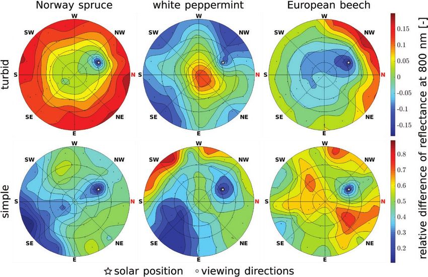
(2021). The latter approach of Stovall et al. (2021) also performs the tance is underestimated between −12 % and −18 %. The Norway12 • Janoutová et al.
Downloaded from https://academic.oup.com/insilicoplants/article/3/2/diab026/6358408 by guest on 29 October 2021
Figure 8. Comparison of DART-simulated nadir reflectance signatures of three scenarios for each investigated species. The
scenarios vary in tree abstractions: (i) 3D detailed tree representations (3D detailed), (ii) 3D detailed tree representation
transformed into a turbid medium (turbid) and (iii) predefined simple tree crown shapes filled with a turbid medium and
simplified trunks (simple). At the bottom row are relative differences from the 3D detailed reference scenario.Detailed reconstruction from TLS for RS apps • 13
spruce and European beech turbid scenarios are overestimated at reflectance is overestimated around nadir viewing angles by about
the extreme zenith viewing angles by 5 % up to 15 %. The white 13 % and underestimated in extreme zenith viewing angles by about
peppermint turbid scenario demonstrates a different behaviour, its −12 %. In all three cases of simple scenarios, the relative difference
shows reflectance overestimation, with the hot spot region being
overestimated by around 11 %. Additionally, reflectance of simple
scenarios differs from the reference of 3D detailed forest abstrac-
tions more heterogeneously across simulated viewing angles than
turbid scenarios.
The differences in simulated reflectance of three forest abstractions
show that the reconstruction of a 3D detailed tree representation plays
an important role in achieving accurate airborne and satellite spectral
Downloaded from https://academic.oup.com/insilicoplants/article/3/2/diab026/6358408 by guest on 29 October 2021
data simulations. The tree abstraction using predefined simple tree
crown shapes filled with a turbid medium and simplified trunks is unable
to reliably substitute the 3D detailed tree representation. The reflectance
differences were also noticeable when the 3D detailed tree representa-
tions were converted in a canopy turbid medium. However, the con-
version into turbid medium saves time and decreases computational
demands (summarized in Table 7), e.g. in case of spruce scene the 3D
detailed scenario took 12 h and 33 min with 155 GB RAM at 30 CPU to
Figure 9. Relative difference of DART-simulated nadir scene be simulated, while the turbid scenario needed only 1 h and 59 min with
reflectance between the reference 3D detailed scenario and 21 GB RAM at 20 CPU. In some applications, this might be a sufficient
two simpler scenarios (turbid and simple) for each species. justification for trading the reflectance accuracy by the computational
Description of scenarios is available in the caption of Fig. 8. feasibility.
Figure 10. Relative differences in multi-angular distribution of simulated forest canopy reflectance at 800 nm between the
complex scenario with 3D detailed tree abstractions (3D detailed) and the two simpler scenarios. Description of the simpler
scenarios is available in the caption of Fig. 8.14 • Janoutová et al.
Table 7. DART model computational demands for simulating The second example presents a virtual sensitivity study inves-
forest scenes of three species: Norway spruce, white tigating impact of wooden canopy parts (trunks and branches)
peppermint and European beech. on SIF of white peppermint forest stands simulated in DART
(Gastellu-Etchegorry et al. 2017). Because it is physically impos-
Parameter 3D detailed Turbid Simple
sible to remove wood and measure the effect of its absence or
Product Simulated forest bidirectional reflectance factors presence in a real forest, the RT computer simulations were the
between 400 and 800 nm with a step of 10 nm only way to achieve this objective (Malenovský et al. 2020, 2021).
Computation 30 CPU 20 CPU 10 CPU Three-dimensional tree representations of four white peppermint
demands [per 155–7 GB 22–11 GB RAM 62–24 GB trees (Fig. 6) were used to create four DART virtual scenes: (i)
simulation] RAM RAM a dense stand (ground CC about 80 %) containing wood (trunk
753–35 min 120–48 min 394–184 min and branches), (ii) the same stand without wood (only leaves),
Downloaded from https://academic.oup.com/insilicoplants/article/3/2/diab026/6358408 by guest on 29 October 2021
DART version 5.7.9. v1192 (iii) a sparse stand (CC about 40 %) containing wood and (iv)
the same sparse stand without wood. Subsequently, RTMs were
employed to simulate SIF signals, as observed by an airborne RS
3.3 RS applications sensor above a forest canopy, and also a portion of SIF photons
Some optical RS applications are deeply rooted in computer-based escaping from the canopy in all directions and in the nadir view-
RTMs that simulate light interactions (absorption and scattering) with ing direction. Comparison of the outcomes for simulations with
3D objects placed inside a virtual scene (e.g. Liu et al. 2019b; Lukeš and without wood enabled us to reveal wood’s potential impact.
et al. 2020; Malenovský et al. 2021). Such modelling requires structural Appendix B provides a detailed description of the methodology
representations of the studied objects that are sufficiently detailed to and its results.
enable RTM to resolve light interactions at spatial scales appropriate The future perspective of this work entails a combination of TLS
to specific research questions ( Janoutová et al. 2019; Malenovský et al. data with, or even its replacement by, airborne laser scanning (ALS)
2020, 2021). Numerous RS RTM-based applications, such as simula- measurements. A larger spatial extent of ALS acquisitions would
tion of terrestrial and airborne laser scans for validation and calibration allow for efficient reconstruction of entire forest stands. As suggested
of above-ground forest biomass estimations (Disney et al. 2018) or scal- by Jurík (2019), the ALS data could be used to segment a forest into
ing of leaf optical signals to the top of forest canopies (Malenovský et al. individual trees and then to select the best performing tree 3D recon-
2019; Lukeš et al. 2020), require reconstructed 3D abstractions of trees. struction for each detected tree from a library based on species and
In Appendices A and B, we provide two case studies as exam- tree proportions (e.g. tree height, crown width and shape). Use of ALS
ples demonstrating use of the 3D tree representations created in data requires new methods capable of creating individual tree 3D rep-
this work for (i) interpretation of airborne and space-borne spec- resentations from point clouds of much lower density, but it represents
tral RS data and (ii) investigating influence of forest structures, par- a significant step forward towards fully automated reconstruction of
ticularly woody components, on remotely sensed SIF signal. Both large virtual forest stands.
applications are computationally highly demanding procedures.
To reduce their computational time, the 3D tree representations 4. C O N C LU S I O N
had to be created from a minimal number of required geometri- The algorithm, originally developed for detailed 3D reconstruction
cal facets. Inasmuch as the original algorithm outputs were con- from TLS scans of coniferous Norway spruce trees, was success-
structed from far too many facets (Table 6), we separated the part fully extended and applied to two broadleaf tree species, white pep-
distributing the foliage objects within a tree crown as a stand-alone permint and European beech. The extension required a few simple
algorithm. This offered a quick and easy way to replace the foliage modifications of the previous algorithm, but no significant changes
objects with others having an optimal lower number of facets (see had to be introduced. Although the reconstruction proved to be
Table 3) whenever needed. robust and applicable to the three species of this study, it requires
The first example shows retrievals of biophysical parameters of further testing, especially for tree species of irregular shapes grow-
Norway spruce forest stands at the Bílý Kříž study site (Table 1 and ing in extreme environmental conditions (e.g. high-altitude tree-
Fig. 1) from hyperspectral RS images (Fig. 12) by means of an RTM lines or high-latitude boreal forests).
inversion (Fig. 11). The 3D spruce representations of this study Our detailed 3D representations of trees with complex archi-
(Fig. 5) were used to create a set of about 20 000 forest scenes, tectures improved existing and enabled new RS applications and
reassembling the existing forest architecture and biochemistry sensitivity studies that were unfeasible using previous, much sim-
variations (Table 8), and to simulate in DART their reflectance pler tree abstractions. This capability is highly relevant for syner-
spectral signatures as measured from airborne sensors. A support gistic use of imaging unmanned aircraft systems operating at very
vector regression algorithm was then trained with the DART sim- high spatial resolutions of only a few centimetres. With the rapid
ulations and subsequently applied on real hyperspectral airborne development of ALS RS techniques and improving performance
images of the study site to quantify contents of leaf chlorophylls, of computational resources, it might soon be possible to recon-
carotenoids and water, as well as LAI (Fig. 13). Appendix A pro- struct and simulate even whole forest stands of a given study area.
vides a detailed methodological description and results of this A fundamental prerequisite for achieving this goal is a fully auto-
case study. mated algorithm for reconstructing trees.Detailed reconstruction from TLS for RS apps • 15
S U P P O RT I N G I N F O R M AT I O N IGARSS 2018—2018 IEEE International Geoscience and Remote
The following additional information is available in the online version Sensing Symposium, 2869–2872, Valencia, Spain. doi:10.1109/
of this article— IGARSS.2018.8519208.
Figure S1. Visualization of Norway spruce forest 3D scenes and DART- Barták M. 1992. Struktura koruny smrku ztepilého ve vztahu k produkci.
simulated top-of-canopy reflectance images for three scenarios. Brno, Czechoslovakia: Kandidátská dizertační práce, Ústav system-
Figure S2. Visualization of white peppermint forest 3D scenes atické a ekologické biologie, Československá akademie věd.
and DART-simulated top-of-canopy reflectance images for three Barták M, Dvořák V, Hudcová L. 1993. Rozložení biomasy jehlic v koru-
scenarios. nové vrstvě smrkového porostu. Lesnictví, 273–281. Praha: ÚVTIZ.
https://www.muni.cz/vyzkum/publikace/196846.
Figure S3. Visualization of European beech forest 3D scenes and
Bienert A, Georgi L, Kunz M, Maas H-G, Von Oheimb G. 2018.
DART-simulated top-of-canopy reflectance images for three scenarios.
Comparison and combination of mobile and terrestrial laser scan-
Downloaded from https://academic.oup.com/insilicoplants/article/3/2/diab026/6358408 by guest on 29 October 2021
ning for natural forest inventories. Forests 90:395.
Blender Online Community. 2017. Blender—a 3d modelling and ren-
A C K N O W L E D G E M E N TS dering package. Amsterdam: Stichting Blender Foundation. http://
The authors would like to thank Petr Sloup and Tomáš Rebok www.blender.org.
from the Masaryk University in Brno for providing code for Bremer M, Rutzinger M, Wichmann V. 2013. Derivation of tree skel-
3D tree wooden parts reconstruction; Luke Wallace and etons and error assessment using LiDAR point cloud data of vary-
Samuel Hillman from the RMIT University in Melbourne ing quality. ISPRS Journal of Photogrammetry and Remote Sensing
for acquisition of the white peppermint TLS point clouds; 80:39–50.
and IFER–Institute of Forest Ecosystem Research, Ltd. and Calders K, Disney MI, Armston J, Burt A, Brede B, Origo N, Muir J,
Nightingale J. 2017. Evaluation of the range accuracy and the
IFER–Monitoring and Mapping Solutions, Ltd. for provid-
radiometric calibration of multiple terrestrial laser scanning instru-
ing the field data for the Těšínské Beskydy study site. Jean- ments for data interoperability. IEEE Transactions on Geoscience and
Philippe Gastellu-Etchegorry, Nicolas Lauret and members Remote Sensing 550:2716–2724.
of the DART team at the CESBIO Laboratory in Toulouse Calders K, Newnham G, Burt A, Murphy S, Raumonen P, Herold M,
are acknowledged for supporting our DART modelling. We Culvenor D, Avitabile V, Disney M, Armston J, Kaasalainen M.
also thank three anonymous reviewers for their constructive 2015. Nondestructive estimates of above-ground biomass using
comments that helped us to improve this manuscript. terrestrial laser scanning. Methods in Ecology and Evolution
60:198–208.
Chianucci F, Pisek J, Raabe K, Marchino L, Ferrara C, Corona P. 2018.
SOURCE OF FUNDING
A dataset of leaf inclination angles for temperate and boreal broad-
This work was supported by the Ministry of Education, Youth and Sports of
leaf woody species. Annals of Forest Science 750:50.
Czech Republic within the CzeCOS program (grant no. LM2018123) and
CloudCompare (version 2.9). 2017. CloudCompare - 3D point cloud
within the Inter-Excellence program (grant no. LTC20055) and by the Action
and mesch processing software, Open Source Project. https://
CA17134 SENSECO (‘Optical synergies for spatiotemporal sensing of scal- www.cloudcompare.org/.
able ecophysiological traits’) funded by COST (European Cooperation in Correa-Díaz A, Silva LCR, Horwath WR, Gómez-Guerrero A, Vargas-
Science and Technology, www.cost.eu). The contribution of Z.M. was funded Hernández J, Villanueva-Díaz J, Velázquez-Martínez A, and Suárez-
by the Australian Research Council Future Fellowship ‘Bridging Scales in Espinoza J. 2019. Linking remote sensing and dendrochronology
Remote Sensing of Vegetation Stress’ (FT160100477). to quantify climate-induced shifts in high-elevation forests over
space and time. Journal of Geophysical Research: Biogeosciences
C O N F L I C TS O F I N T E R E ST 1240:166–183.
None declared. Danson FM. 1998. Teaching the physical principles of vegetation can-
opy reflectance using the SAIL model. Photogrammetric Engineering
C O N T R I BU T I O N S BY T H E AU T H O R S & Remote Sensing 64:809–812.
R.J., L.H. and Z.M. contributed to the conception and design of the work; Darenova E, Pavelka M, Macalkova L. 2016. Spatial heterogeneity of
CO2 efflux and optimization of the number of measurement posi-
R.J., J.N., B.N. and M.P. collected and processed the data; R.J., L.H. and
tions. European Journal of Soil Biology 75:123–134.
Z.M. contributed to data analysis and interpretation; R.J. performed
Disney MI, Boni Vicari M, Burt A, Calders K, Lewis SL, Raumonen P,
modelling and conducted the simulations; R.J., L.H. and Z.M. contrib-
Wilkes P. 2018. Weighing trees with lasers: advances, challenges
uted to drafting the manuscript; L.H. and Z.M. supervised the imple-
and opportunities. Interface Focus 8:20170048.
mentation and contributed to critical revision of the manuscript. Disney M, Lewis P, Saich P. 2006. 3D modelling of forest canopy struc-
ture for remote sensing simulations in the optical and microwave
domains. Remote Sensing of Environment 1000:114–132.
L I T E R AT U R E C I T E D
Fabrika M, Scheer U, Sedmák R, Kurth W, Schön M. 2019. Crown
Abdelmoula H, Kallel A, Rouiean L, Chaabouni S, Gargouri K, architecture and structural development of young Norway spruce
Ghrab M, Gastellu-Etchegorry J, Lauret N. 2018. Olive biophysi- trees (Picea abies Karst.): a basis for more realistic growth model-
cal property estimation based on Sentinel-2 image inversion. In: ling. BioResources 140:908–921.You can also read