DPPD: Deformable Polar Polygon Object Detection
←
→
Page content transcription
If your browser does not render page correctly, please read the page content below
DPPD: Deformable Polar Polygon Object Detection
Yang Zheng Oles Andrienko Yonglei Zhao Minwoo Park Trung Pham
NVIDIA
{yazheng, oandrienko, yongleiz, minwoop, trungp}@nvidia.com
arXiv:2304.02250v1 [cs.CV] 5 Apr 2023
Abstract
Regular object detection methods output rectangle bound-
ing boxes, which are unable to accurately describe the ac-
tual object shapes. Instance segmentation methods output
pixel-level labels, which are computationally expensive for
real-time applications. Therefore, a polygon representation
is needed to achieve precise shape alignment, while retain- Figure 1. For crosswalk detection, polygon shapes are in green;
ing low computation cost. We develop a novel Deformable bounding boxes are in red. It is clear that bounding boxes are unable
Polar Polygon Object Detection method (DPPD) to detect to represent the crosswalk regions well as compared to polygons.
objects in polygon shapes. In particular, our network pre-
dicts, for each object, a sparse set of flexible vertices to
construct the polygon, where each vertex is represented by
a pair of angle and distance in the Polar coordinate system.
To enable training, both ground truth and predicted poly-
gons are densely resampled to have the same number of ver-
tices with equal-spaced raypoints. The resampling operation
is fully differentable, allowing gradient back-propagation.
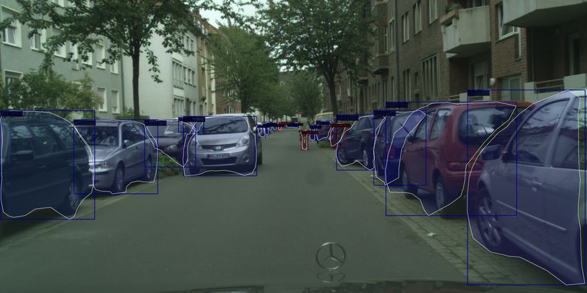
Sparse polygon predicton ensures high-speed runtime infer- Figure 2. Example of approximating ground truth polygons (green)
ence while dense resampling allows the network to learn using polar polygons (red) with fixed angular bins. Notice that 64
object shapes with high precision. The polygon detection rays is still insufficient to capture the actual crosswalk regions.
head is established on top of an anchor-free and NMS-free
network architecture. DPPD has been demonstrated suc-
cessfully in various object detection tasks for autonomous be run much faster than a segmentation network plus post-
driving such as traffic-sign, crosswalk, vehicle and pedes- processing. Unfortunately, polygon detection is more com-
trian objects. plex than box detection in the variant numbers of vertices
of arbitrary shapes. This creates difficulties when training a
network to predict a fixed number of vertices. A common
1. Introduction solution (e.g., as done in previous methods such as Polar-
Mask [25]) is that ground truth polygons are represented in
Object detection, as one of the most popular computer Polar coordinates and approximated by a vector of distance
vision tasks, typically predicts objects in rectangle bounding values and a (fixed) vector of evenly-spacing angular values.
boxes. Boxes are able to describe locations and sizes, but The task becomes training a network to regress, for each ob-
not object shapes. Fig. 1 shows an example of crosswalk ject, a radius vector, together with the predefined uniformly
detection for autonomous driving, where precise crosswalk emitted rays decoded back to polygon. A clear limitation of
regions are needed. This can be achieved by an instance this method is that the quality of ground truth labels (and
segmentation method which outputs a pixel-wise mask per thus the quality of prediction) is bounded by the number of
object. However, pixel-level post-processing is computation- rays. Fig 2 shows that even with 64 rays, crosswalk regions
ally expensive, thus not suitable for real-time applications. are not well captured. Increasing the numbers of rays will
Alternatively, a method that detects objects as polygons increase the computational cost significantly.
is a better choice because 1) polygons can capture object In this work, we propose a novel Deformable Polar Poly-
shapes with high accuracy, and 2) a detection network can gon Object Detection method, namely DPPD. Unlike Polar-
1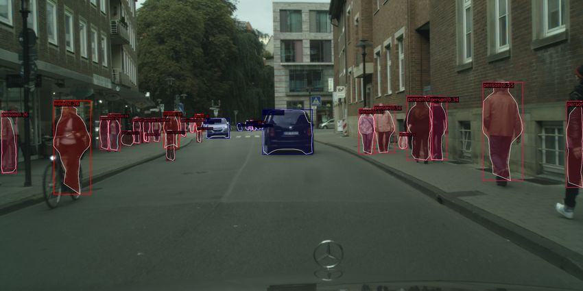
Figure 3. An illustration of the deformable polygon shape learning process. The target shape is in blue, and the predicted shape with 24
vertices is in red. From iteration step 1 to 200 to 500, the predicted shape is converging close to the target.

Mask, our network predicts a small set of flexible polygon             16, 19], to anchor-free and NMS-free detectors [6, 23, 28],
vertices directly, where each vertex has two degrees of free-          transformer-based detectors [3], and other variations [1,9,14,
dom in Polar coordinates, i.e., radius and angle. Intuitively,         17, 18]. In general, an object detector includes three major
starting from an initialized polygon, the network will deform          components: a backbone of series of convolutional blocks, a
it until it aligns well with the ground truth polygon (see Fig.        neck of multi-resolution feature pyramids [13], and a de-
3). A question arises is how to compare and compute loss be-           tection head. The detection head is usually divided into
tween ground truth and prediction where they are different in          a classification head and a bounding box regression head.
the number of vertices. Our idea is to densely resample both           Our detection method follows the anchor-free, NMS-free ap-
ground truth and prediction with a certain number of rays.             proach, but the box regression head is replaced by a polygon
We could resample as many rays as the memory allows. It’s              regression head to predict object locations and boundaries.
worth emphasizing that the resampling process only happens
                                                                           Instance Segmentation. Instance segmentation produces
at the loss computation, thus does not affect the inference
                                                                       pixel-level class-ids and object-ids. Mask R-CNN [8] intro-
runtime, and that the resampling operation is differentiable,
                                                                       duces a detect-then-segment approach to breakdown this
allowing gradient based optimization.
                                                                       problem into two sequential sub-tasks. To overcome the
    Note that DPPD is designed for polygon shape regression,           expensive two-stage processing, YOLOACT [2] and its ex-
and it is applicable for any successful object detection archi-        tended methods [4, 22, 24] construct a parallel assembling
tecture. In this work, we establish a high-speed, single-shot,         framework, by generating a set of prototype masks and pre-
anchor-free, NMS-free detection network structure based on             dicting per-instance mask coefficients. However, regardless
set prediction [20, 27] and build DPPD on top of it. This              of model variations, the per-pixel segmentation mask output
simple architecture escalates both training effectiveness and          is always a huge burden for downstream real-time applica-
inference efficiency.                                                  tions.
    The main contributions of this work can be summarized
as follows: 1) We propose a novel polygon detection method                 Polygon Detection. A series of work, such as Ex-
to detect objects with arbitrary shapes. Our method avoids             tremeNet [29], ESE-Seg [26], PolarMask [25], and Fourier-
a trade-off decision between network computation cost and              Net [21], try to parameterize the contour of an object mask
polygon accuracy as in PolarMask; 2) a method to decode a              into fixed-length coefficients, given different decomposi-
regression vector into a valid polygon (e.g., vertices are in          tion bases. These methods predict the center of each object
counter-clockwise order), a batching processing algorithm to           and the contour shape with respect to that center. Polar-
resample sparse polygons to dense polygons with a minimum              Mask is the one closest to our method, which is built on
cost; 3) Inspired by the latest object detection development,          top of FCOS [23] and utilizes depth-variant rays at con-
we design a highly efficient single-stage, anchor-free and             stant angle intervals. Similarly, PolyYOLO [10] adopts the
NMS-free polygon detection architecture; 4) Our proposed               YOLOv3 [18] architecture, and modifies the perpendicular
polygon detector surpasses previous polygon detection meth-            grid into circular sectors to detect polar coordinates of poly-
ods in both speed and accuracy when tested on autonomous               gon vertices. Each circular sector is responsible to produce 1
driving perception tasks such as crosswalk, road sign, vehicle         or 0 vertex. The drawback of these methods is that the shape
and pedestrian detection.                                              alignment quality is heavily bottlenecked by the pre-defined
                                                                       ray bases. Increasing the number of rays is possible to im-
2. Related Work                                                        prove the quality, but meanwhile downgrading the speed
                                                                       performance. In contrast, our method is less dependent on
   Object Detection. Object detection has been evoluted                the number of vertices. We found that as small as 12 vertices
from two-stage or one-stage anchor-based detectors [15,                is sufficient to model variety of object shapes.

                                                                   2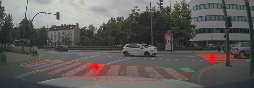
Figure 4. Overall network architecture and training pipeline. We establish a classification head and a regression head to generate N candidates.
The N candidates are matched with M groundtruths, resulting in M pairs of prediction-target assignments. Based on the assignment, we
compute positive classification and regression losses.

    Active Contour Model (ACM). In the classical com-                      3.2. Polygon Regression
puter vision area, the active contour model [11] has been
                                                                           3.2.1                 Polar Representation
used to describe object shape boundaries. The main idea
is to minimize an dedicated internal and external energy                   In the polar coordinates, each polygon is represented as one
functions. The external term is to control the contour shape               origin (object center) and k pairs of radial distances and
fitting, and the internal term is to control the deformation               polar angles. Distances and angles are defined w.r.t the ob-
continuity. Our DPPD is inspired by the ACM. The training                  ject center. The network will output a (2 + 2 ∗ k)-vector,
loss jointly minimizes the shape fitting error between ground              where 2 values are for the polygon origin and 2 ∗ k values
truth and prediction polygons and polygon smoothness.                      are for k vertices. The contouring vertices, in the polar rep-
                                                                           resentation, are convenient to be organized a clockwise or
                                                                           counterclockwise order.
3. Method
   In this section, we first introduce the overall set prediction          3.2.2                 Polygon Decoding
network architecture. We then describe the polygon detection               The decoding process parses a regression output vector
head. And lastly, we discuss the training strategies.                      [f0 , f1 , ..., f2∗k+2 ] to the corresponding polygon origin co-
                                                                           ordinates, radial distances, and polar angles, denoting as
3.1. Object Detection as Set Prediction                                    [ox , oy , r0 , ..., rk−1 , a0 , ..., ak−1 ].
                                                                               Polygon origin In the fully convolutional set prediction
    We adopt an anchor-free and NMS-free set prediction                    framework, every grid cell at the feature map yields a candi-
approach for our DPPD object detector due to its simplic-                  date. To get the accurate location, we predict offsets w.r.t. the
ity and efficiency. The network predicts a set of N candi-                 grid cell position. Formally, the polygon origin is decoded
dates (N ≫ M number of ground truth objects). The N                        as:                      \begin {aligned} \begin {cases} o_{x} = g_{x} + s_{x} * \sigma (f_{0}) \\ o_{y} = g_{y} + s_{y} * \sigma (f_{1}) \end {cases} \end {aligned} \label {eq:3}
candidates are matched with M ground truth labels using
                                                                                                                                                                                                                                                    (1)
a Hungarian matching algorithm, resulting in M pairs of
prediction-target assignments. Classification and regression
losses from these matches are computed to supervise the                    where (ox , oy ) denote the polygon origin coordinates;
training. For unmatched candidates, only classification loss               (gx , gy ) denote the grid cell coordinates; (sx , sy ) denote
is computed.                                                               the grid cell size; σ is a sigmoid activation function.
                                                                               Radial distances The next k regression outputs
   Fig. 4 depicts the high-level network architecture and
                                                                           (f2 , ..., fk+2 ) are dedicated for k radial distances. The de-
training pipeline. Followed by the network backbone and
                                                                           coding function is:
feature pyramid is a classification head and a regression head.
The regression head predicts polygon origins (i.e., object                                                                    \begin {aligned} r_{i} = \mu * e^{f_{i}}, i \in [2, k+2] \end {aligned} \label {eq:4}                                 (2)
center) and vertices (i.e., radial distance and polar angles).
One grid cell in the feature map is responsible for detecting              where µ is a prior knowledge of the radius scale. We apply
one polygon candidate.                                                     an exponential activation to ensure the decoded radius is

                                                                       3
always positive.
Polar angles The last k output channels
(fk+2 , ..., f2∗k+2 ) are responsible for the k polar an-
gles. We predict angle deltas between adjacent vertices, and
then decode using cumulative sum before normalizing them
into [0, 2π] range:
\begin {aligned} a_{i} = 2 \pi * \dfrac {\sum _{j=k+2}^{i}e^{f_{j}}}{\sum _{j=k+2}^{2*k+2}e^{f_{j}}}, i \in [k+2, 2*k+2] \end {aligned} \label {eq:5} (3)
(a) Triangle approach. (b) Vector approach.
It can be seen clearly that unlike the previous methods
such as PolarMask [25], which predefined polar angles (e.g., Figure 5. O is the polygon center, A and B are two adjacent vertices,
⃗ is one ray emitted from O. The goal is to find the intersection
OR
by shooting uniform rays from 0 to 360 degrees), our method ⃗ Refer to Sec. 3.3.2
point P between the segment AB and ray OR.
predicts both polar angles and radial distances. This allows
for detailed derivation.
the network to deform the initial polygons as much as needed
to match the ground truth polygons. In contrast, previous
methods find difficulties to fit well the ground truth shapes m rays. To simplify the computation, we assume the poly-
unless a dense number of rays (e.g., 360) is used. gon is translated to its origin at (0, 0). In polar coordinates,
Note that the angle decoder also differentiates DPPD since rays are uniformly emitted with the same angle inter-
against Poly-YOLO [10]. Poly-YOLO splits the polar coor- val, the resampling output only consists a m dimensional
dinates into circular sectors where each sector is responsible radial distance vector [r0 , r1 , ..., rm−1 ]. We provide two ap-
for either 1 (exist) or 0 (non-exist) vertex. This design is un- proaches to tackle this problem, triangle approach and vector
able to discriminate clustered vertices that fall into the same approach.
sector. Instead, DPPD predicts angle deltas, which could be Triangle Approach. In Fig. 5a, let A and B be two ad-
small and large to handle arbitrary intervals. jacent vertices and O be the origin. The task is to find the
intersection point P between segment AB and ray OR. ⃗ The
3.3. Training
norm | · | notation is used for the segment length. Deriving
3.3.1 Ground Truths from the triangle similarity between △ACP and △BDP :
Objects are often annotated using polygons. However, there
is no consistent way to enforce all the objects having the \begin {aligned} w = \dfrac {|AP|}{|BP|} = \dfrac {|AC|}{|BD|} = \dfrac {|OA|\sin (\alpha )}{|OB|\sin (\beta )}. \end {aligned} \label {eq:6} (4)
same number of vertices and vertex distributions along the
boundaries. Therefore, it is less reasonable to train a network we compute a length ratio w between |AP | and |AB|.
to predict polygons with a fixed number of vertices and by Then the point P coordinates are calculated as:
directly comparing ground truth and predicted vertices as
often done in the box regression problem. \begin {aligned} (P_x, P_y) = (\dfrac {A_x + w B_x}{1+w}, \dfrac {A_y + w B_y}{1+w}). \end {aligned} \label {eq:7} (5)
Instead, we propose a simple method to tackle this is-
sue, in which both ground truth and prediction polygons The coordinates of O, A, B and their segment lengths are
are resampled to have the same number of points, namely known from the decoding outputs. OR ⃗ is one of the m equal-
raypoints. Bear in mind that this resampling process only spaced resampling rays. Given a list of polygon vertices with
happens during training, thus does not hinder inference la- their sorted polar angles, we can easily find, for each ray, a
tency. This simple idea seems overlooked in the past mainly pair of neighboring vertices A, B via linear search so that
because the resampling operation might be not efficient, and the ray locates between OA⃗ and OB.⃗
not differentiable for SGD based training. Below we will Vector Approach. In Fig. 5b, for each known segment
describe two resampling methods which are both efficient AB and ray OR,⃗ let define the following 4 vectors:
and differentiable.
\begin {aligned} \begin {cases} \vec {v_1} = (\vec {OR}_x, \vec {OR}_y) \\ \vec {v_2} = (B_x - A_x, B_y - A_y) \\ \vec {v_3} = (-\vec {OR}_y, \vec {OR}_x) \\ \vec {v_4} = (O_x - A_x, O_y - A_y) \end {cases} \end {aligned} \label {eq:unit_vectors}
3.3.2 Polygon Resampling
(6)
Given a polygon with k vertices, we want to upsample it
with m (m > k) raypoints along equally distributed po-
lar angles. This resampling process is a geometry problem,
i.e., to find intersections between k boundary segments and ⃗ and AB, we
Since P is the intersection point by OR
4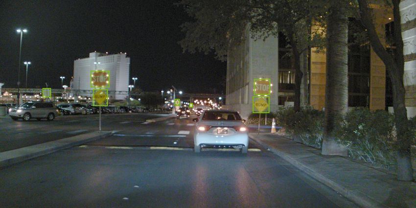
⃗ and AP
formulate the vector representation of OP ⃗ : height, [xo , yo ] be the prediction center, the origin loss is
\begin {aligned} \begin {cases} \vec {OP} = O + t_{1}\vec {v_{1}}, t_{1} \in [0, \infty ) \\ \vec {AP} = A + t_{2}\vec {v_{2}}, t_{2} \in [0, 1] \end {cases} \end {aligned} \label {eq:8} computed as:
(7) \begin {aligned} \mathcal {L}_{o} = \dfrac {l^s_1(o_{x}, \hat {o}_{x})}{\hat {w}} + \dfrac {l^s_1(o_{y}, \hat {o}_{y})}{\hat {h}} \end {aligned} \label {eq:11} (11)
⃗ Polar IoU loss. The polar IoU loss Liou measures shape
where t1 and t2 are the fractional scale of units along OR
⃗ difference between the two polygons regardless of their lo-
and AB. Finding the intersection is to solve t1 and t2 from
cations. Let [r̂0 , r̂1 , ..., r̂m−1 ] and [r0 , r1 , ..., rm−1 ] be the
Eq. (7). We constrain t1 ∈ [0, ∞) to ensure P is along the
ground truth and prediction radial distances respectively, the
⃗ and t2 ∈ [0, 1] to ensure P is
positive direction of ray OR, polar IoU loss is computed as:
inside segment AB. The mathematical solution is:
\begin {aligned} \begin {cases} t_{1} = \dfrac {|\vec {v_{2}} \times \vec {v_{4}}|}{\vec {v_{2}} \cdot \vec {v_{3}}} \\ t_{2} = \dfrac {\vec {v_{4}} \cdot \vec {v_{3}}}{\vec {v_{2}} \cdot \vec {v_{3}}} \end {cases} \end {aligned} \label {eq:9} \begin {aligned} \mathcal {L}_{iou} = \log \dfrac {\sum _{i=0}^{m-1}\max (r_{i}, \hat {r_{i}})}{\sum _{i=0}^{m-1}\min (r_{i}, \hat {r}_{i})} \end {aligned} \label {eq:12} (12)
(8)
Smoothness loss. The smoothness loss is added to reduce
the shape oscillation, similar to the internal energy of the
classical active contour model [11]. Let [r0 , r1 , ..., rm−1 ] be
where the operator · is the dot product and × is the cross the prediction radial distances, d1 r and d2 r be the 1st and
product. Suppose v⃗1 is decomposed into [v1x , v1y ], combin- 2nd ordered differences, the smoothness loss is computed as:
ing Eq. (7), the coordinates of P is written as:
\begin {aligned} \mathcal {L}_{sm} = \dfrac {\sum _{i=1}^{m-1}d^1r_i}{m-1} + \dfrac {\sum _{i=1}^{m-1}d^2r_i}{m-1} \end {aligned} \label {eq:13} (13)
\begin {aligned} (P_x, P_y) = (O_{x} + t_{1} v_{1x}, O_{y} + t_{1} v_{1y}). \end {aligned} \label {eq:10} (9)
Note that the triangle approach assumes vertices have
been ordered ascendingly. For predictions, we decode polar 4. Experiment
angles in counter-clockwise order, which naturally satisfies
We conduct experiments using two datasets: our in-house
the assumption. However, for ground truth encoding, this is
autonomous driving dataset, and the public Cityscapes [5]
not guaranteed for concave shapes. Therefore, the triangle
dataset. Since one major application of the polygon detector
approach is only used for prediction decoding. On the other
is for autonomous driving perception, we use our in-house
hand, the vector approach has no requirements on the ver-
dataset for the primary investigation. We focus on road-sign
tex order, and it works for both convex and concave shapes.
and crosswalk detections where accurate object boundaries
However, the cross-product calculation expense much mem-
are important for subsequent tasks such as localization, sign
ory in the practical implementation, therefor vector approach
recognition. We examine the effectiveness of polygon detec-
is only used for ground truth encoding.
tors against bounding box detectors, and thoroughly compare
DPPD with PolarMask [25] in terms of both accuracy and
3.3.3 Polygon Regression Losses speed performance. To further demonstrate the generic effec-
tiveness, we benchmark DPPD results on Cityscapes, which
A common way to measure the loss between two shapes covers more dynamic instances like vehicles and pedestrians.
is based on their intersection-over-union (IoU). For general We also explore ablation studies for the model design.
polygons, there is no exact closed-form solution. Fortunately,
with the polar representation and the above resampling strat- 4.1. DPPD on Internal Datasets
egy, computing losses between ground truth and prediction The in-house dataset statistics for road sign and crosswalk
polygons becomes easier. Formally, the polygon shape re- are summarized in Table 1, where all labels are given as
gression loss Lreg is a weighted sum of three components: polygon vertices. In this experiment, we establish DPPD
polygon origin loss Lo , polar IoU loss Liou and internal polygon head on top of a FPN augmented AlexNet network
smoothness loss Lsm : backbone. The number of channels for different CNN blocks
are 32, 128, 256, 512 respectively. The input image size is
\begin {aligned} \mathcal {L}_{reg} = w_{1}\mathcal {L}_{o} + w_{2}\mathcal {L}_{iou} + w_{3}\mathcal {L}_{sm} \end {aligned} \label {eq:10} (10) 960 × 480. The feature maps at stride 8 and 32 are used for
the crosswalk and road-sign tasks separately.
Polygon origin loss. The origin loss Lo measures the dif-
ference between two polygons’ centers. We employ smooth-
4.1.1 Polygon vs Bounding Box
l1 loss (l1s ) for the absolute distance error. Also the losses are
normalized by the ground truth size. Formally, let [x̂o , ŷo ] We first demonstrate the polygon detector is substitute for
be the ground truth center, [ŵ, ĥ] be the polygon width and the bounding box detector. Typically, road signs are detected
5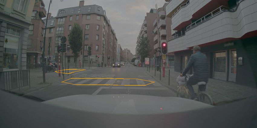
Figure 6. Two examples to visualize bounding box (left) and DPPD polygon (right) detections on traffic-signs. The polygon detector is better
to capture the object shape.

Table 1. Number of instances for traffic-sign and crosswalk polygon       Table 2. Traffic-sign results. Box vs. polygon detector. Accuracy
detection datasets.                                                       metrics precision (P ), recall (R), F1-score (F 1) are in percentages.
                                                                          The speed is measured as latency times on Titan GPU and Orin
                 Task       Training    Evaluation                        Chip devices, in ms.

              Road sign      377.4K        39.6K
                                                                                Detector       P         R         F1       GPU      Chip
              Crosswalk      260.2K        36.1K
                                                                                  BBox       74.91      58.68     65.81     1.54     3.18
                                                                                 Polygon     74.54      57.31     64.80     1.63     3.05
as bounding boxes. To swap it with a polygon model, we
ensure that the new polygon model has non-negative effects
on both detection accuracy and inference latency.                         Table 3. Crosswalk results. PolarMask vs. DPPD. The accuracy is
   In this experiment, we set the number of predictable ver-              evaluated based on polygon IoU directly. The speed is measured as
tices k = 12, and the number of resampling rays m = 180.                  latency times on GPU and Chip devices, in ms.
To compare the polygon against the box model, we convert
polygons to their envelop bounding boxes, and evaluate both                     Detector           P         R       F1       GPU      Chip
detectors based on the box metrics. Results are listed in Ta-                 PolarMask-36      61.58     38.00     47.00       -        -
ble 2. It shows that the polygon model is on-par with the box                 PolarMask-64      66.72     45.46     54.08     1.91     3.24
model with a very slight regression, although the polygon                       DPPD-36         77.27     50.46     61.05     1.28     2.68
model was not trained to detect boxes. Nevertheless, the
polygon model produces tighter alignments to the objects,
which are qualitatively visualized in Fig. 6.
   The speed performance is device-dependent. We measure                  i.e., 36 and 64. Since crosswalk shapes are more complex,
the runtime inference latency (in ms) when the model is                   the matching criteria is based on polygon-to-polygon IoU di-
deployed to TensorRT and run in FP16 precision on two                     rectly. Metrics results and visualizations are shown in Table 3
hardware platforms: 2080 Titan GPU, and NVIDIA DRIVE                      and Fig. 7 respectively.
Orin chip. The polygon detector runs 0.09ms slower on                        In terms of accuracy, DPPD is superior than PolarMask
GPU, while 0.13ms faster on the chip. We consider the                     in all metrics, even the number of predictable vertices is
inference time is comparable on both platforms. This is                   less in DPPD (36) than PolarMask (64). The first reason is
expected because only the last regression layer is changed,               that PolarMask ground truth are approximated radius length
whereas the change of regression channels is minor w.r.t. the             along pre-defined rays, which are not guaranteed to reach
total number of model parameters.                                         ”real” vertices (e.g., Fig. 2). The second reason is that DPPD
                                                                          predicts, for each vertex, both radial distance and polar angle,
4.1.2   DPPD vs PolarMask                                                 which allows greater capability to achieve high-quality shape
                                                                          regression.
Next we emphasize the benefits of DPPD against the state-
of-the-art polygon detectors. We pick PolarMask as our                       In terms of the speed, DPPD also costs less inference time
competitor, and use the crosswalk detection task for this                 than PolarMask on both platforms. We claim it is benefitted
experiment. In DPPD, we set the number of prediction ver-                 from the design of separate training and inference features.
tices k = 36, and the number of resampling rays m = 360.                  Dense polygons for training facilitates the accuracy, and
In PolarMask, we experimented different number of rays,                   sparse polygon for inference boosts the runtime speed.

                                                                      6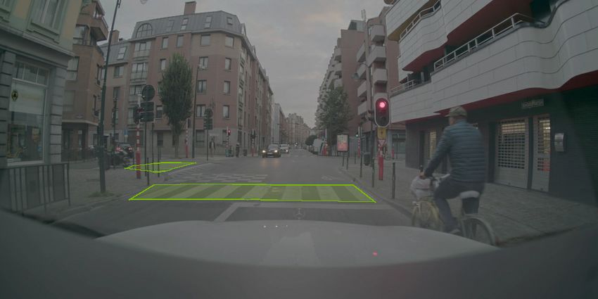
Figure 7. Two examples to visualize 64-vertex PolarMask (left) and 36-vertex DPPD (right) results on crosswalks. DPPD expenses less
vertices but achieves tighter alignment with the groundtruth.

                                 Figure 8. Qualitative visualizations of DPPD results on Cityscapes.

4.2. DPPD on Public Dataset                                           Table 4. Benchmark on Cityscapes. Poly-YOLO predicts 24 ver-
                                                                      tices, whereas DPPD predicts 12 vertices. YOLOv3 and Poly-
    To examine the generic effectiveness, we experiment               YOLO use DarkNet53 backbone, whereas MaskRCNN and DPPD
DPPD on the public Cityscapes [5] dataset, which covers               use ResNet50 backbone.
more dynamic objects like vehicles, pedestians, bicycles, etc.
We pick Poly-YOLO (an improved version of PolarMask                           Method            Detector   AP      AP50    FPS
and YOLOv3) as our main competitor. As the Poly-YOLO                      YOLOv3 [18]             Box      10.6    26.6    26.3
used DarkNet-53 as the backbone, we select Resnet50 as the                MaskRCNN [8]            Mask     16.4    31.8     6.2
backbone for our DPPD for a fair comparison. Input resolu-
                                                                        Poly-YOLO [10] (24)      Polygon    8.7    24.0    21.9
tion is 1024 × 2048. we set the number of prediction vertices
                                                                             DPPD (12)           Polygon   11.96   27.31   56.1*
k = 12, and the number of resampling rays m = 360. Re-
sults of DPPD is based on the official Cityscapes evaluation
metrics at the instance level, tested on the validation split.
Results of other methods are borrowed from the Poly-YOLO              from approximated labels. Poly-YOLO is trained for boxes
paper [10].                                                           and polygons jointly, and it is claimed benefited from the
                                                                      auxiliary task learning. However, it predicts the object cen-
    As shown in Table 4, for the accuracy, DPPD surpasses
                                                                      ter for both box and polygon, which is not guaranteed well
the state-of-the-art polygon method Poly-YOLO, even using
                                                                      aligned (see Fig. 9). On the other hand, DPPD is a polygon-
a smaller number of vertices predicted (12 vs. 24). Qualita-
                                                                      only detector. The resampling process allows DPPD to learn
tive visualization are shown in Fig. 8. For the speed, DPPD
                                                                      from the real polygon shape without any approximation, the
runs at 56.1 FPS, measured on a Tesla V100 GPU. Since
                                                                      angle decoding method enables its capability to fit for both
it is hard to reproduce competitors latency from the exact
                                                                      sparse and dense vertices, and the object center encoded as
same environment, we mark it with a * symbol to indicate
                                                                      the geometry centroid.
reference purpose only.
    Poly-YOLO is built as an extension of YOLOv3. Compar-             4.3. Ablation Studies
ing with DPPD, there are many fundamental differences such
as the backbone structure, target assignment mechanisms,                 Admittedly, the optimization of model structure, data
loss functions, etc. Considering the polygon head itself, due         augmentation, and other fantastic training strategies could
to the fact of circular grid splits, Poly-YOLO is still learned       further improve the overall performance. But in this sub-

                                                                  7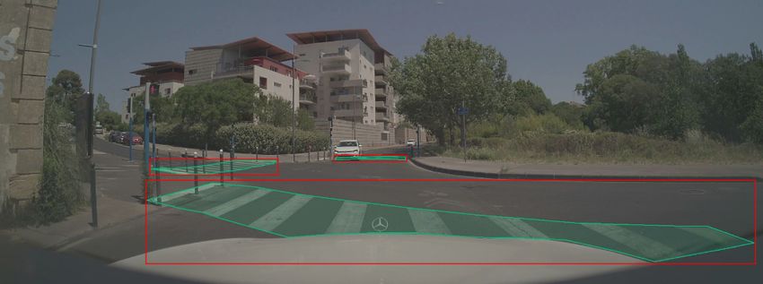
Table 5. Ablation studies for DPPD design choices.

        Exp.     Dataset     Origin Finding     Angle Decoder    # of Vertices   # of Rays    P       R      F1      AP      AP50
          1     Crosswalk      box center         bin offsets         36           360       69.19   50.22   58.20     -       -
          2     Crosswalk    vertices mean        bin offsets         36           360       50.13   49.89   50.01     -       -
          3     Crosswalk     geo centroid        bin offsets         36           360       72.02   54.54   62.08     -       -
          4     Cityscapes    geo centroid        bin offsets         18           360         -       -       -     11.10   25.80
          5     Cityscapes    geo centroid         cumsum             18           360         -       -       -     12.01   27.45
          6     Cityscapes    geo centroid         cumsum             12           120         -       -       -     10.38   24.17
          7     Cityscapes    geo centroid         cumsum             12           180         -       -       -     11.54   27.29
          8     Cityscapes    geo centroid         cumsum             12           360         -       -       -     11.96   27.31
          9     Cityscapes    geo centroid         cumsum             18           360         -       -       -     12.01   27.45
         10     Cityscapes    geo centroid         cumsum             36           360         -       -       -     11.67   26.83

section, we focus on the key components involved in the
polygon detector regression head. Specifically, we discuss
the design choices of polygon origin finding methods, angle
decoding methods, number of prediction vertices, number of
resampling rays.
   Polar Origin Finding. The polygon polar origin holds
two regression targets. To find the groundtruth, we consid-
ered three methods: (i) the mean of all vertices; (ii) the
bounding box center that covers the polygon; (iii) the poly-
gon shape geometry centroid. However, (i) and (ii) are un-
able to guarantee that the polar origin is located within the              Figure 9. Example of polygon polar origin finding. If the vehicle
polygon boundary (see Fig. 9), which voids the model effec-                object is partially occluded, the bounding box center (green) is
tiveness. Therefore, (iii) geometry centroid is the only choice.           outside of the polygon shape boundary (red).
We run experiments on a subset of crosswalk objects and
compared the three methods, shown as Exp. 1-3 in Table 5.                  and instance segmentation. The polygon detector is able to
   Angle Decoding. The flexible angle prediction is one ma-                describe precise object shape information, while retaining
jor distinction of DPPD. Comparing against PolarMask [25],                 fast runtime inference speed. Our polygon detection method
this is the second degree of freedom of each vertex; com-                  is able to predict object shapes with high accuacy without
paring against Poly-YOLO [10], it breaks the angle sector                  a need to use an excessively large number of vertices as
constraint. Using the Cityscapes data, we experiment two                   done in the previous methods. This is possible due to our
angle decoding methods: (i) predict an offset within each                  novel polygon training strategy, in which both ground truths
angle bin; (ii) the angle cumulative summation. According                  and predictions (not necessarily having the same number of
to Exp. 4-5 in Table 5, (ii) obtains higher accuracy than (i).             vertices) are up-sampled so that both have the same number
   Predictable Vertices and Resampling Rays. The num-                      of raypoints. The upsampling (resampling) is efficient and
ber of predictable vertices and resampling rays are important              differentiable, which is required for training. From the ex-
hyperparameters to construct the DPPD head. We experi-                     periments using both in-house autonomous driving dataset
ment six combinations of vertices and rays on Cityscapes.                  and public dataset, DPPD outperforms PolarMask and Poly-
Results are listed in Table 5. Increasing the number of rays               YOLO in terms of both accuracy and speed for many detec-
(Exp.6 - 8) results in the accuracy improvement, this is ex-               tion tasks such as road sign, crosswalk, car, pedestrian.
pected since we have denser representation of the polygon                      Although DPPD is designed as a 2D polygon detector, it
shape. On the other hand, increasing the number of vertices                is also applicable in 3D perception. Many state-of-the-art 3D
(Exp.8 - 10) is less effective. Keep increasing it will lead to            detectors adopt BEV [12] or rangeview [7] representations
excessive model complexity and hence lower generalization                  for runtime efficiency. We could place DPPD on top of any
capability. But this is a good indicator that DPPD is able to              detection architecture for complex shape understanding.
achieve promising results even with less regression outputs.
                                                                           References
5. Conclusion
                                                                            [1] Alexey Bochkovskiy, Chien-Yao Wang, and Hong-Yuan Mark
   In this paper, we present DPPD, a deformable polygon                         Liao. Yolov4: Optimal speed and accuracy of object detection.
detector that stands intermediately between object detection                    arXiv preprint arXiv:2004.10934, 2020. 2

                                                                       8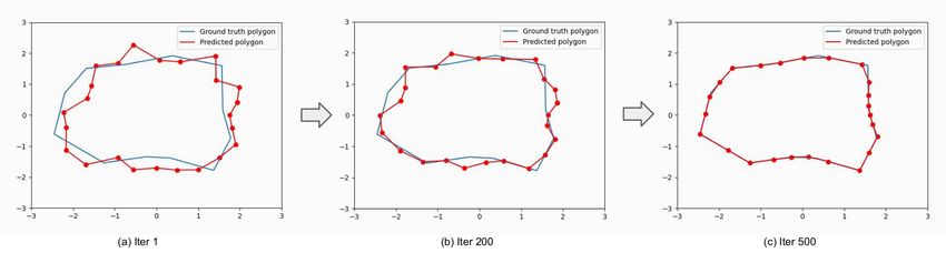
[2] Daniel Bolya, Chong Zhou, Fanyi Xiao, and Yong Jae Lee.                      ceedings of the IEEE international conference on computer
     Yolact: Real-time instance segmentation. In Proceedings of                   vision, pages 2980–2988, 2017. 2
     the IEEE/CVF international conference on computer vision,             [15]   Wei Liu, Dragomir Anguelov, Dumitru Erhan, Christian
     pages 9157–9166, 2019. 2                                                     Szegedy, Scott Reed, Cheng-Yang Fu, and Alexander C Berg.
 [3] Nicolas Carion, Francisco Massa, Gabriel Synnaeve, Nicolas                   Ssd: Single shot multibox detector. In European conference
     Usunier, Alexander Kirillov, and Sergey Zagoruyko. End-                      on computer vision, pages 21–37. Springer, 2016. 2
     to-end object detection with transformers. In European con-           [16]   Joseph Redmon, Santosh Divvala, Ross Girshick, and Ali
     ference on computer vision, pages 213–229. Springer, 2020.                   Farhadi. You only look once: Unified, real-time object de-
     2                                                                            tection. In Proceedings of the IEEE conference on computer
 [4] Hao Chen, Kunyang Sun, Zhi Tian, Chunhua Shen, Yong-                         vision and pattern recognition, pages 779–788, 2016. 2
     ming Huang, and Youliang Yan. Blendmask: Top-down meets               [17]   Joseph Redmon and Ali Farhadi. Yolo9000: better, faster,
     bottom-up for instance segmentation. In Proceedings of the                   stronger. In Proceedings of the IEEE conference on computer
     IEEE/CVF conference on computer vision and pattern recog-                    vision and pattern recognition, pages 7263–7271, 2017. 2
     nition, pages 8573–8581, 2020. 2                                      [18]   Joseph Redmon and Ali Farhadi. Yolov3: An incremental
 [5] Marius Cordts, Mohamed Omran, Sebastian Ramos, Timo                          improvement. arXiv preprint arXiv:1804.02767, 2018. 2, 7
     Scharwächter, Markus Enzweiler, Rodrigo Benenson, Uwe                [19]   Shaoqing Ren, Kaiming He, Ross Girshick, and Jian Sun.
     Franke, Stefan Roth, and Bernt Schiele. The cityscapes                       Faster r-cnn: Towards real-time object detection with region
     dataset. In CVPR Workshop on the Future of Datasets in                       proposal networks. Advances in neural information process-
     Vision, volume 2. sn, 2015. 5, 7                                             ing systems, 28, 2015. 2
 [6] Kaiwen Duan, Song Bai, Lingxi Xie, Honggang Qi, Qingming              [20]   Hamid Rezatofighi, Tianyu Zhu, Roman Kaskman, Farbod T
     Huang, and Qi Tian. Centernet: Keypoint triplets for object                  Motlagh, Javen Qinfeng Shi, Anton Milan, Daniel Cremers,
     detection. In Proceedings of the IEEE/CVF international                      Laura Leal-Taixé, and Ian Reid. Learn to predict sets using
     conference on computer vision, pages 6569–6578, 2019. 2                      feed-forward neural networks. IEEE Transactions on Pattern
 [7] Lue Fan, Xuan Xiong, Feng Wang, Naiyan Wang, and Zhaoxi-                     Analysis and Machine Intelligence, 44(12):9011–9025, 2021.
     ang Zhang. Rangedet: In defense of range view for lidar-based                2
     3d object detection. In Proceedings of the IEEE/CVF Inter-            [21]   Hamd Ul Moqeet Riaz, Nuri Benbarka, and Andreas Zell.
     national Conference on Computer Vision, pages 2918–2927,                     Fouriernet: Compact mask representation for instance seg-
     2021. 8                                                                      mentation using differentiable shape decoders. In 2020 25th
 [8] Kaiming He, Georgia Gkioxari, Piotr Dollár, and Ross Gir-                   International Conference on Pattern Recognition (ICPR),
     shick. Mask r-cnn. In Proceedings of the IEEE international                  pages 7833–7840. IEEE, 2021. 2
     conference on computer vision, pages 2961–2969, 2017. 2, 7            [22]   Zhi Tian, Chunhua Shen, and Hao Chen. Conditional convo-
 [9] Rachel Huang, Jonathan Pedoeem, and Cuixian Chen. Yolo-                      lutions for instance segmentation. In European conference on
     lite: a real-time object detection algorithm optimized for non-              computer vision, pages 282–298. Springer, 2020. 2
     gpu computers. In 2018 IEEE International Conference on               [23]   Zhi Tian, Chunhua Shen, Hao Chen, and Tong He. Fcos: Fully
     Big Data (Big Data), pages 2503–2510. IEEE, 2018. 2                          convolutional one-stage object detection. In Proceedings of
[10] Petr Hurtik, Vojtech Molek, Jan Hula, Marek Vajgl, Pavel                     the IEEE/CVF international conference on computer vision,
     Vlasanek, and Tomas Nejezchleba. Poly-yolo: higher speed,                    pages 9627–9636, 2019. 2
     more precise detection and instance segmentation for yolov3.          [24]   Yuqing Wang, Zhaoliang Xu, Hao Shen, Baoshan Cheng, and
     Neural Computing and Applications, 34(10):8275–8290,                         Lirong Yang. Centermask: single shot instance segmentation
     2022. 2, 4, 7, 8                                                             with point representation. In Proceedings of the IEEE/CVF
[11] Michael Kass, Andrew Witkin, and Demetri Terzopoulos.                        conference on computer vision and pattern recognition, pages
     Snakes: Active contour models. International journal of                      9313–9321, 2020. 2
     computer vision, 1(4):321–331, 1988. 3, 5                             [25]   Enze Xie, Peize Sun, Xiaoge Song, Wenhai Wang, Xuebo
[12] Zhiqi Li, Wenhai Wang, Hongyang Li, Enze Xie, Chonghao                       Liu, Ding Liang, Chunhua Shen, and Ping Luo. Polarmask:
     Sima, Tong Lu, Yu Qiao, and Jifeng Dai. Bevformer: Learn-                    Single shot instance segmentation with polar representation.
     ing bird’s-eye-view representation from multi-camera images                  In Proceedings of the IEEE/CVF conference on computer
     via spatiotemporal transformers. In Computer Vision–ECCV                     vision and pattern recognition, pages 12193–12202, 2020. 1,
     2022: 17th European Conference, Tel Aviv, Israel, October                    2, 4, 5, 8
     23–27, 2022, Proceedings, Part IX, pages 1–18. Springer,              [26]   Wenqiang Xu, Haiyang Wang, Fubo Qi, and Cewu Lu. Ex-
     2022. 8                                                                      plicit shape encoding for real-time instance segmentation. In
[13] Tsung-Yi Lin, Piotr Dollár, Ross Girshick, Kaiming He,                      Proceedings of the IEEE/CVF International Conference on
     Bharath Hariharan, and Serge Belongie. Feature pyramid                       Computer Vision, pages 5168–5177, 2019. 2
     networks for object detection. In Proceedings of the IEEE             [27]   Yan Zhang, Jonathon Hare, and Adam Prugel-Bennett. Deep
     conference on computer vision and pattern recognition, pages                 set prediction networks. Advances in Neural Information
     2117–2125, 2017. 2                                                           Processing Systems, 32, 2019. 2
[14] Tsung-Yi Lin, Priya Goyal, Ross Girshick, Kaiming He, and             [28]   Xingyi Zhou, Dequan Wang, and Philipp Krähenbühl. Objects
     Piotr Dollár. Focal loss for dense object detection. In Pro-                as points. arXiv preprint arXiv:1904.07850, 2019. 2

                                                                       9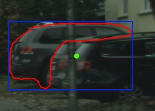
[29] Xingyi Zhou, Jiacheng Zhuo, and Philipp Krahenbuhl.
     Bottom-up object detection by grouping extreme and center
     points. In Proceedings of the IEEE/CVF conference on com-
     puter vision and pattern recognition, pages 850–859, 2019.
     2

                                                                  10
You can also read