E2 distribution and statistical regularity in polygonal planar tessellations
←
→
Page content transcription
If your browser does not render page correctly, please read the page content below
E2 distribution and statistical regularity in polygonal planar
                                                                                                       tessellations
                                                                           Ran Li1 , Consuelo Ibar2 , Zhenru Zhou2 , Seyedsajad Moazzeni1 ,
arXiv:2002.11166v2 [cond-mat.stat-mech] 5 Nov 2020

                                                                                 Kenneth D. Irvine2∗, Liping Liu1,3†, and Hao Lin1‡

                                                                                                      November 9, 2020

                                                     1. Department of Mechanical and Aerospace Engineering, Rutgers, The State University of New Jersey
                                                     2. Waksman Institute and Department of Molecular Biology and Biochemistry, Rutgers, The State
                                                     University of New Jersey
                                                     3. Department of Mathematics, Rutgers, The State University of New Jersey

                                                                                                            Abstract

                                                                 From solar supergranulation to salt flat in Bolivia, from veins on leaves to cells on Drosophila
                                                             wing discs, polygon-based networks exhibit great complexities, yet similarities persist and statistical
                                                             distributions can be remarkably consistent. Based on analysis of 99 polygonal tessellations of a wide
                                                             variety of physical origins, this work demonstrates the ubiquity of an exponential distribution in the
                                                             squared norm of the deformation tensor, E2 , which directly leads to the ubiquitous presence of Gamma
                                                             distributions in polygon aspect ratio. The E2 distribution in turn arises as a χ2 -distribution, and an
                                                             analytical framework is developed to compute its statistics. E2 is closely related to many energy forms,
                                                             and its Boltzmann-like feature allows the definition of a pseudo-temperature. Together with normality
                                                             in other key variables such as vertex displacement, this work reveals regularities universally present in
                                                             all systems alike.

                                                     Polygonal networks are one of nature’s favorite ways of organizing the multitude - from supergranulation
                                                     on the solar surface [29] to cracked dry earth [37]; from ice wedges in northern Canada [61] to the scenic
                                                     Salar de Uyuni in Bolivia [23]; and from veins on leaves [11] to cells on Drosophila wing discs [53] (Fig. 1).
                                                     These systems are driven by distinctive physical mechanisms, yet they share common features. Individual
                                                     constituents, namely, “cells” appear to “randomize” into statistical distributions, and only interact with
                                                     their immediate neighbors. On the collective level, especially in the dynamic and active systems, rich
                                                     phenomena are observed, including unjamming and jamming, fluid-to-solid phase transition, and flow and
                                                     migration [7, 19, 22, 34, 42, 50, 54, 63, 68].
                                                           Despite the complexity and variabilities involved in these phenomena, similarity patterns emerge. One
                                                     particularly interesting instance is provided recently by Atia et al. [3]. Within the context of confluent
                                                     biological tissue and based on extensive experiments both in vitro and in vivo, the authors found that data
                                                       ∗
                                                         Corresponding email: irvine@waksman.rutgers.edu
                                                       †
                                                         Corresponding email: liu.liping@rutgers.edu
                                                       ‡
                                                         Corresponding email: hlin@soe.rutgers.edu

                                                                                                                1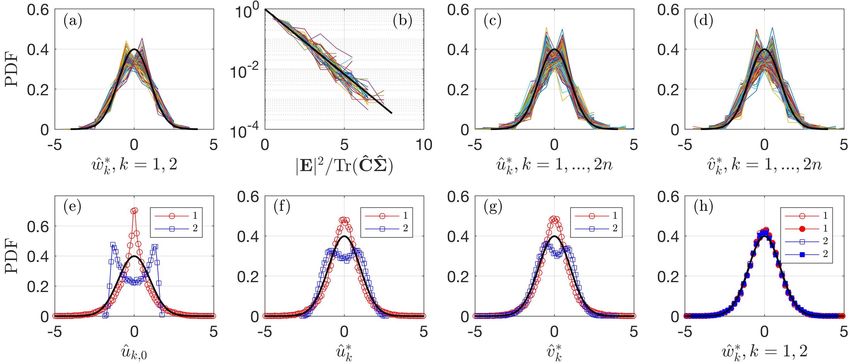
3
                                                                                                      Aspect Ratio
                                                                                                      1    2
Figure 1: (a)-(h) Examples of randomized polygonal networks in nature. (a) Land cracks due to desiccation
[37]; (b) Ice wedges from northern Canada [61]; (c) Veins on a Ficus lyrata leaf [11]; (d) Desiccation
pattern of an ancient lake on Mars [43]; (e) A snapshot of Salar de Uyuni in Bolivia, world’s largest salt
flat [23]; (f) Supergranulation on solar surface [29]; (g) Plated MDCK cells (this work). (h) A processed
image of a developing Drosophila wing disc (this work) with the aspect ratio of cells color-mapped. (i) A
regular hexagon PR (blue, with vertices xj ), a deformed hexagon P (red, with vertices yj ), and a uniform
deformation as mean-field approximation P 0 (black dashed outline, with vertices yj0 ).

on cell aspect ratio collapse and follow a normalized Gamma distribution, implying a universal principle
underlying the geometric configuration and pertinent processes.
   What is the basis of this universality? Does it carry beyond the biological context? This work composes
of a two-part discovery to answer these questions. In the first, we analyze a total of 99 data sets in 8
groups that include convection patterns (solar supergranulation), landforms (salt flats, on Mars, and in
or near the Arctic), cracked dry earth, and biological patterns (veins on leaves, cells on Drosophila wing
discs, and plated MDCK cells). (Fig. 1 and Table 1.) We demonstrate that the Gamma distribution
in polygon aspect ratio derives from an exponential distribution in the squared strain tensor norm, E2 ,
based on which we develop a unifying solution for the former. Both distributions persist in all data
examined. In the second, we tackle the origin of the E2 distribution, and demonstrate that it arises as a
χ2 -distribution owing to asymptotic normality of vertex displacement and other key variables. We present
a theoretical framework to accurately compute E2 from vertex statistics. Importantly, E2 is closely related
to various definitions of system energy including all of the bulk-, perimeter-, and moment-based (known
as the Quantizer) forms [7, 15, 27, 34, 36, 44]. The Boltzmann-like feature of E2 enables the definition of
a pseudo-temperature that can be considered as a consistent quantifier [4, 17, 18, 47]. The exponential
and normal distributions we reveal in this work are hidden regularities that transcend the specific physical
systems, and are embedded universal features of random polygonal tessellations.

                                                     2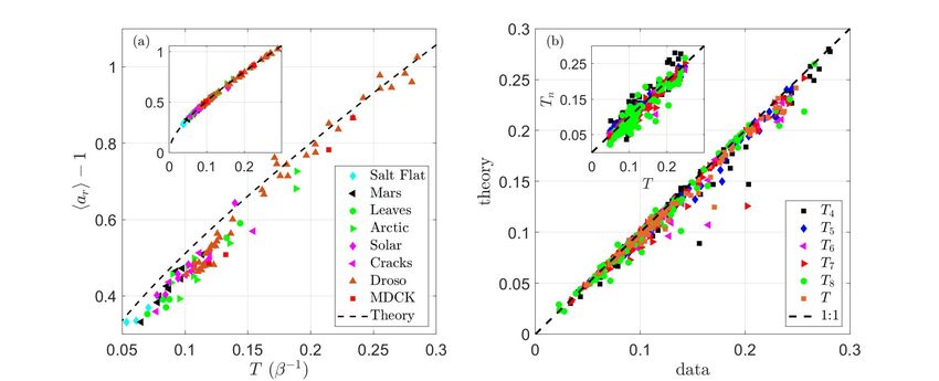
E2 and its relationship with aspect ratio
In this first part of this work, we define E2 and analytically establish its relationship with the polygon
aspect ratio. We demonstrate that a k-Gamma distribution in the latter is derivable from an exponential
distribution in the former. We begin by defining the mean-field deformation tensor, E. An exemplary
processed image of a Drosophila wing disc 120h after egg laying (AEL) is shown in Figure 1h, where the
color scale indicates magnitude of the cell aspect ratio (defined in Methods). We choose as our reference
frame a regular n-polygon centered at the origin, with vertices

                         xj = r0 ej ,     ej = [cos(j2π/n), sin(j2π/n)],           j = 1, ..., n.         (1)

This polygon is denoted by PR , and r0 is a scaling factor. Figure 1k uses n = 6, a hexagon as an illustrative
example. We consequently regard any n-sided polygon P with vertices yj as a “deformation” from PR ,

                                              yj = xj + uj ,     j = 1, ...n.                             (2)

Note that this deformation is to be understood as a morphological deviation from the reference PR , rather
than an actual physical deformation, although the latter is a possibility. We also require that the centroid
of P is aligned with that of PR . The deformation is in general non-uniform, in the sense that for n ≥ 3, a
single deformation tensor of F ∈ R2×2 cannot be identified by yj = Fxj for all of j = 1, ..., n. Nevertheless
we can introduce an approximation, namely,

                                            yj ≈ yj0 = Fxj ,      j = 1, ..., n.                          (3)

This approximation is analogous to a Taylor expansion in which only the leading order term is retained.
The use of a uniform deformation to approximate the local and non-uniform deformation field is effectively
coarse-graining, reducing the degree of freedom from 2n to 4 and suppressing the fluctuations. This idea
is illustrated in Figure 1i (right), where P 0 is the approximate and uniformly deformed polygon. From F
we define the usual strain tensor and its squared Frobenius norm,

                                 1      1
                      E = (FT F) 2 − I ≈ [(F − I) + (F − I)T ],                 |E|2 = Tr(ET E),          (4)
                                        2

where I is the identity tensor, and the approximation in the first equation is valid in the small-to-moderate
deformation regime. In this work we use |E|2 (mathematical representation) and E2 (terminology) inter-
changeably. The restriction to isochoric (area-conserved) deformation requires that det F = 1 and equiv-
alently (to leading order), TrE = 0, which is satisfied by choosing r0 in (1). Consequently, E has a small
degree of freedom of 2, which eventually leads to its strong regularity that we demonstrate later.
   We pursue an analytical expression for E via minimizing the difference between yj ’s and yj0 ’s in (3),
from which we obtain (SI)
                                              n
                                     1X
                                  E=   [vj ⊗ ej + ej ⊗ vj − (ej · vj )I],                                 (5)
                                     n
                                             j=1

                             n X
                               n
                             X                                 2
                    |E|2 =             vi · Cij vj ,   Cij =      [(ei · ej )I + ej ⊗ ei − ei ⊗ ej ].     (6)
                                                               n2
                             i=1 j=1

                                                           3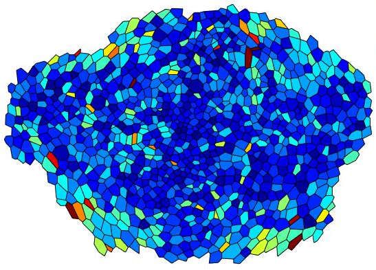
Here
n
1X
vj = uj /r0 , r0 = yj · ej . (7)
n
j=1
In addition to satisfying the trace-free condition, the scaling also ensures that vj ’s are dimensionless.
Further details on the computation of |E|2 is deferred until later. For now we show that if E2 follows an
exponential distribution (that shall be validated below both via data and analysis), namely,
ρE (|E|2 ) = β exp(−β|E|2 ), (8)
then the aspect ratio follows a k-Gamma distribution such as shown in [3]. Here ρ(·) denotes a (normalized)
probability density function (PDF), and β is similar to an inverse temperature as the PDF is Boltzmann-
like. The aspect ratio ar of the polygon is calculated via the second area moments (Methods), and is
related to E2 by (SI)
a2r = (x + 1)2 = g(|E|2 ), g(t) = 1 + 2t2 + 4t + [(2t2 + 4t + 1)2 − 1]1/2 , (9)
where for convenience we define a shape factor x in relation to ar using x = ar − 1. Based on (8, 9), a
transformation ρE (|E|2 )d|E|2 = ρX (x)dx leads to
d|E|2
ρX (x) = ρE (|E|2 ) = βζ 0 (x) exp(−βζ(x)), (10)
dx
where
ζ(x) = g −1 ((x + 1)2 ).
Here we have considered the normalization condition. Equation (10) is our prediction of the distribution
in the aspect ratio.
Data validate E2 and ar distributions
Both distributions and their relationship are extensively validated with a total of 99 data sets spanning 8
groups summarized in Table 1; detailed descriptions, data sources, and method of analysis are presented
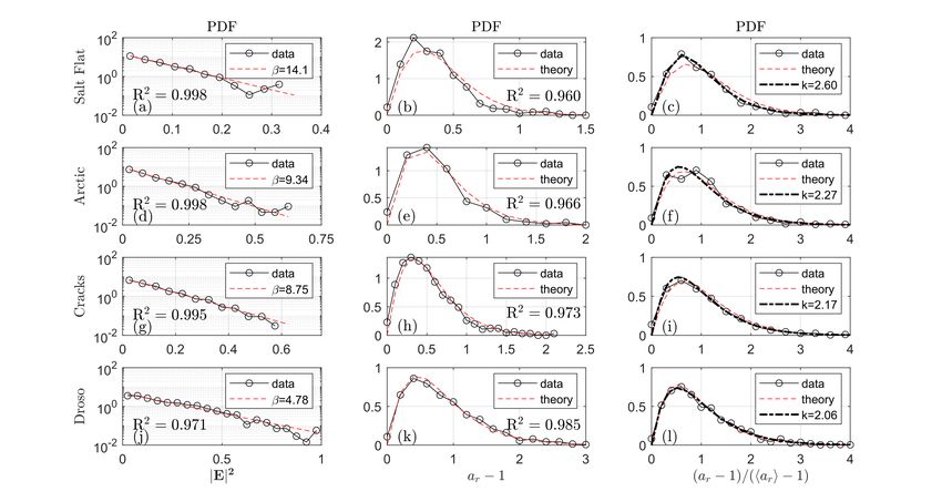
in the Methods section. Figure 2 uses 4 representative cases to demonstrate the agreement. (More are
shown in Fig. S2 in the SI.) The left column shows the PDFs of |E|2 , which are very well fitted by the
exponential form, exp(−β|E|2 ), where β is extracted as a fitting parameter. (See also Fig. 4b where all
|E|2 profiles are presented and the value of β is theoretically predicted.)
The center column shows the PDFs of the shape factor, ar − 1 (symbols). The theoretical predictions
per Eq. (10) are shown in dashed, and exhibit excellent agreement with data. They are generated per Eq.
(10), with the single input parameter, β, extracted from the analysis of |E|2 distribution.
Lastly in the right column, the PDFs for ar − 1 are normalized with har i − 1, where h·i denotes a mean,
e.g.,
ˆ ∞
hxi = xρX (x)dx. (11)
0
Both data and theoretical predictions are normalized following this practice. The dot-dashed are best fits
4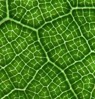
Type (abbreviation)                    M             N           R2 , |E|2       R2 , ar − 1
          Salt Flat of Uyuni (Salt Flat)              7         193 − 849    0.994 ± 0.0058   0.939 ± 0.0255
           Landforms on Mars (Mars)                   9        219 − 5826    0.986 ± 0.0125   0.935 ± 0.0461
             Veins on Leaves (Leaves)                 6        338 − 6050    0.994 ± 0.0047   0.936 ± 0.0328
         Landforms in the Arctic (Arctic)             11       104 − 1061    0.982 ± 0.0169   0.902 ± 0.0728
     Supergranulation on Solar Surface (Solar)        9        192 − 1645    0.991 ± 0.0075   0.932 ± 0.0463
           Cracked Dry Earth (Cracks)                 11       298 − 1596    0.992 ± 0.0067   0.943 ± 0.0353
          Drosophila Wing Disc (Droso)                42       902 − 4205    0.991 ± 0.0083   0.955 ± 0.0335
          Plated MDCK Cells (MDCK)                    4        1148 − 2283   0.997 ± 0.0012   0.936 ± 0.0157

Table 1: Summary of data for a total of Mtot = 99 tessellations. Abbreviations are defined within
parentheses and are used in figure legends; M is data sets in each type; N , the number of polygons in each
set (range provided). R2 for |E|2 indicates quality of fitting (e.g., in left column, Fig. 2); R2 for ar − 1
indicates quality of agreement between theory and data (e.g., in middle column, Fig. 2). Data sources are
presented in Methods.

using a k-Gamma distribution defined as

                                                       k k k−1
                                     ρkG (x1 ; k) =        x   exp(−kx1 ),                                     (12)
                                                      Γ(k) 1

where Γ(k) is the Gamma function, and k is the single fitting parameter. The agreement is evident, and
the k-values are found to vary between 2 and 3.
   Overall corroboration between theory and data is quantified by the coefficient of determination, R2 ,
and are listed in Table 1 for all cases (see Methods for definition). The values are uniformly close to 1
(“perfect agreement”) with minimal variations from case to case. Validity of the theoretical prediction (10)
is also attested by Fig. 3a. Here we define a pseudo temperature T as the inverse of β, namely, T = β −1 .
To compare with data, a theoretical prediction is generated by using (10) in the integration (11).
   The above results validate that the E2 does follow an exponential, Boltzmann-like distribution. The
universality of this distribution in all data sets, according to our theory, necessarily leads to a universality
of k-Gamma distributions for the aspect ratio. That is, the validity extends beyond the confluent tissues
studied in [3], and to all systems we analyzed. As a corollary, (10) provides a fundamental solution for the
aspect ratio, of which the k-Gamma distributions (12) are convenient approximations. This solution does
not normalize to a single curve with a single k value if fitted with Gamma distributions. In fact, it predicts
a positive correlation between β and k (Fig. S8). Qualitatively, this means that PDFs of aspect ratio
(ar , or equivalently, x) with wider spread and greater mean (corresponding to lower values of β) present
themselves relatively to the left after normalization (corresponding to lower values of k and noting that
maxima occur at 1 − 1/k per (12)). This trend is fully corroborated with data from our own work (Fig. 2,
and Fig. S2 in SI, center and right columns) and Atia et al. [3] (Fig. 3 therein), as well as predictions from
a self-propelled Voronoi model in the supplemental information of the latter. In summary, the variability
in k arises from the variability in β.
   We remark that the agreement between our theoretical prediction and data can be even better if we
use a variation of the deformation tensor computed as the square-root of the area moment tensor, M, via
Eq. (21) in the Methods section. This is not surprising, as now both E and ar share the same origin, the
agreement shown in Fig. 3a inset is near perfect. The slight differences between the two definitions are

                                                           5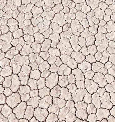
Figure 2: Universality in strain and aspect ratio distributions. Left column shows the PDFs of |E|2 , fitted
with an exponential form exp(−β|E|2 ) to extract β. This β value is used in Eq. (10) to generate the
theoretical curves in the middle column (dash), in comparison to the aspect ratio data (symbols). The
coefficients of determination, R2 are shown within the panels. Right column: both data and theoretical
curves from the center column are normalized using the mean values, and fitted with a k-Gamma function
(12) (thick dashed). A single parameter k is extracted and shown in the figure legends. Data are from
[21], [2], and [60], respectively, for the top 3 rows; and from this work for Droso.

Figure 3: (a) Overall correlation between ar and T ( β −1 ) for all 99 data sets (symbols); the theoretical
prediction (dashed) is generated per (10). The inset alternatively presents E from a moment-based cal-
culation which further improves agreement. (b) A comparison between data and predicted temperature,
Tn and T (“theory”). The inset shows that sub-ensemble temperature Tn ’s are quantitatively similar to
tessellation temperature, T .

                                                     6
due to higher order effects that we theoretically and numerically demonstrate in the SI. Here and below
we focus on using (5) for its apparent analytical simplicity.
E2 distribution is a χ2 -distribution
In the second part of this work, we demonstrate the origin of the highly regular statistical distribution in
E2 . Figure 3b shows results comparing the pseudo-temperature computed from Eq. (6) (denoted “data”)
with the theoretical prediction we develop below (denoted “theory”). Here the subscript n denotes a
restriction to the sub-ensemble of n-gons, Tn := |E|2 n
. Polygons other than n = 4-8 are of statistically
insignificant occurrences and not included in the evaluation.
The key relationship we utilize is a quadratic form to compute |E|2 given vertex displacement, vj ,
|E|2 = v̂ · Ĉv̂. (13)
Here v̂ is a concatenated vector in R2n ,
v̂1 v1
. ..
. (14)
. =
v̂ := .
.
v̂2n vn
Other vectors such as ŷ, û, and ê are similarly defined from their two-dimensional counterparts, and all
vectors and tensors in the 2n-dimensional space are denoted by a hat to differentiate from the planar quan-
tities. Ĉ ∈ Rsym
2n×2n is a second-order tensor with block components C given in (6). Not surprisingly, Ĉ
ij
has 2 non-trivial eigenvalues (SI), matching the degree of freedom of E (note that E = (E11, E12 ; E12 , −E11 )
in a general component form):
P̂T ĈP̂ = diag(2/n, 2/n, 0, ..., 0).
The diagonalization above with the orthonormal tensor P̂ helps us express |E|2 in a particularly simple
form,
2
|E|2 = ŵ12 + ŵ22 , ŵ := P̂T v̂. (15)
n
We realize that ŵk = p̂k · v̂, p̂k being an eigenvector of Ĉ. If v̂ is characterized by a covariance matrix,
Σ̂, then the variance of ŵk is [33]
Var(ŵk ) = p̂k · Σ̂p̂k = Tr(p̂k ⊗ p̂k · Σ̂),
and Tn is readily calculated as
2
Tn = |E|2 n
= Var(ŵ1 + ŵ2 ) = Tr(ĈΣ̂). (16)
n
Note we have used Ĉ = n2 (p̂1 ⊗ p̂1 + p̂2 ⊗ p̂2 ). Here and after and as a good approximation, we assume v̂
has a zero mean. Equation (16) is a precise expression to compute Tn given Σ̂, and is used to generate the
theoretical predictions in Fig. 3b, main panel. The tessellation average T can be computed by taking the
weighted sum of Tn , namely, T = n (Nn Tn )/ n Nn , where Nn is the number of n-gons. On the other
P P
7hand, sub-ensemble temperatures are typically quantitatively similar to the tessellation temperature, as
shown in Fig. 3b inset.
If we further assume that ŵ1,2 follow identical normal distributions, immediately we have
|E|2
1
2
ρE (|E| ) = exp − . (17)
Tn Tn
In other words, the exponential distribution arises actually as a χ2 -distribution with 2 degrees of freedom.
On the other hand, if the variances Var(ŵ1,2 ) are not identical but quantitatively similar, which is true
for all tessellations we study (see Fig. S5), Eq. (17) still holds to the leading order. (This point is
straightforward to prove via Taylor expansion and not shown here for brevity.) Note that even in this
situation, per (16) the formula for Tn is still accurate without approximation. This provides an essential
illustration of the origin of the E2 distribution, and Eq. (17) is a main result of the current work. It
remains to be shown below that ŵ1,2 distributions are indeed approximately normal and independent.
Asymptotic normality contributes to statistical regularity
Fig. 4a presents ŵ1,2 in the hexagon sub-ensemble (n = 6) for all 99 tessellations, whereas the cases for
n = 5 and 7 are included in the SI. PDFs are all normalized for comparison with standard Gaussian, N (0, 1)
(dark solid lines). Although the PDFs exhibit appreciable fluctuations due to the relatively small sample
size in the n-sub-ensemble, the approximate normalities are evident. Quantitative similarities of ŵ1,2 are
demonstrated in Fig. S5. In addition, ŵ1,2 are indeed only weakly dependent, as Cov(ŵ1 , ŵ2 )/Var(ŵ1 ) =
0.078 ± 0.046 for all cases, consistent with the anticipated 2 degrees of freedom. All E2 distributions
(normalized by the predicted temperature Tn ) are shown in Fig. 4b.
The apparent candidate to explain the resulting normality is the central limit theorem in the generalized
version for dependent and identical random variables [39], noting that ŵk derives from v̂k via a linear
combination (15). It is peculiar to note that ûk and v̂k themselves also demonstrate approximate normality,
shown in Fig. 4c and d. The normality in ûk is again be explained by the central limit theorem. We can
write û, the concatenated vector for uj ’s as (SI)
1
û = R̂(ŷ − hŷi), R̂ := Î − ê ⊗ ê.
n
In the absence of apparent anisotropy, components of ŷ − hŷi are approximately dependent yet identical,
satisfying precondition of the theorem. Hence ûk asymptotes to normality. On the other hand, from Eq.
(7) we have v̂ = û/r0 and r0 = (ŷ · ê)/n. The normality in v̂ is difficult to theoretically prove. However, it
is reasonable to speculate the loss of the apparent scale would create similarity to preserve or even enhance
normality - see also Figs 4f, g below. In addition, it is extensively confirmed by the data as shown in Fig.
4d.
The asymptotic normality can be better illustrated via a simple Monte Carlo simulation following
the schematic in Fig. 1k, where we temporarily restrict to an isolated hexagon, and displacements ûk,0
(k = 1, 2, ..., 2n) are prescribed according to independent, identical distributions as shown in Fig. 4e
(Methods, Eqs. (22, 23)). Two representative cases are examined, the first with a steeper than Gaussian
initial descent, and the second non-monotonic. In Figs. 4f and g, both ûk and v̂k already demonstrate
8Figure 4: Normality of key variables. Here the superscript ∗ denotes normalization by its own standard
deviation so as to compare with N (0, 1), the dark line in all panels except for (b) where it represents an
exponential function, exp(·). (a) PDF for ŵk , k = 1, 2, from all tessellations (198 profiles). (b) Normalized
|E|2 follows a simple exponential distribution (99 profiles). (c) and (d) demonstrate the normality of ûk
and v̂k (k = 1, ..., 2n) in the hexagon sub-ensemble (n = 6) , 1188 profiles each. (e) Initial displacement
distributions for two exemplary cases, 1 and 2. (f) and (g) ûk and v̂k asymptote toward normality. (g)
Normalities of ŵ1 and ŵ2 are well-established.
trending toward normality, although some differences from N (0, 1) are still visible. Note only an arbitrary
index k is shown as these distributions are expected to be identical. Subsequently, in Fig. 4h the normality
of ŵ1,2 are well established. |E|2 distribution quantitatively follows our theoretical prediction and is not
shown for brevity. Although only two exemplary tests are presented, repeated simulations reveal the same
asymptotic trend to normality and the quantitative relationships (16, 17) always hold.
In a summary, the above exercises demonstrate that asymptotic normality is prevalent in planar tes-
sellations, as key variables derive from linear combinations of statistically similar components. As a result
E2 distributions become highly regular due to combined normality and its low-dimensionality.
Physical Implications
The physical meaning of E is self-evident: it represents deformation, and hence is typically associated
with energy in one form or another. In the wide range of phenomena we studied, the constitutive relations
come in different forms (some are yet unknown). However, some usual possibilities can be contemplated.
If the energy is bulk-elastic in nature, then any physically reasonable elastic model of a polygon, valid in
the small-to-moderate deformation regime, must follow the form [25]
∆Ψ = µ|E|2 , (18)
where µ is the first Lamé constant, whereas the second constant is not needed as TrE = 0 (SI). On the
other hand, if energy is associated with edge lengths or perimeters, such as in the case of models for 2D
confluent tissues [7, 34, 44], Eq. (18) is still a formally valid approximation, as the change in perimeter is
9also proportional to |E|2 to leading-order approximation (SI). Last but not least, in the Quantizer problem
[15, 27, 36] the cell-wise energy functional is the moment of inertia, which is
TrM = 2m0 (1 + |E|2 ) (19)
in both two and three dimensions (SI), and 2m0 is the moment of inertia of the regular reference polygon,
PR . Thus its distribution can be computed via knowing both the area and E2 distributions. These
examples of constitutive relations cover a reasonably wide range of physical systems.
Above we have taken the liberty in naming a pseudo-temperature, T (or Tn for the sub-ensembles).
Indeed, such definition is both tempting and appropriate in the presence of a Boltzmann-like distribution.
The tests by Dean and Lefèvre [13] and McNamara et al. [47] become trivial: the ratio of two overlap-
ping exponential distributions will necessarily give another exponential distribution. We therefore name
this pseudo-temperature the “E2 temperature”, and propose it as a candidate for a thermodynamically
meaningful temperature owing to its consistent regularity and connection with physical quantities. This
temperature quantifies the overall deformation, and possibly also system energy. To further explore a
thermodynamic framework would require system-specific physical principles, e.g., energy minimization,
which we shall explore in future work.
We have thus demonstrated three main points in this work: i) An exponential distribution in E2 leads
to a k−Gamma distribution in the aspect ratio. In fact, k-Gamma distributions are mere approximations
to the more basic solution we develop. ii) E2 distribution is a χ2 -distribution with two degrees of free-
dom, arising from combined effects of asymptotic normality and the small dimensionality of E, which is
analogous to the small dimensionality of the volume function in granular assembly [8]. We have devel-
oped a formula to compute E2 from vertex statistics. iii) E2 and aspect ratio distributions as well as
normality in displacements are true universal features as we have shown via both a large collection of data
and theoretical derivations illustrating their mechanistic origins. The strong regularity in E2 and vertex
displacements are “hidden patterns” revealed by this work. The mean-field strain tensor, with its clear
physical and geometric meaning, is an ideal quantity connecting the conservation principles, the energy (or
pseudo-energy) landscape, and the geometric distributions. It is a powerful quantifier to describe polygo-
nal networks randomized by active agitations, structural defects, and noises, among others. Analysis may
also be extended to polytopes in three and higher dimensions.
Author contributions
HL, LL, and KDI designed the research; HL, LL, RL, and SM developed the theory; RL, ZZ, and CI
analyzed images; HL, RL, and SM analyzed data; CI and ZZ performed experiments; HL, LL, and KDI
wrote the paper.
Acknowledgement
The authors are grateful to Dr. Yuanwang Pan for providing fixed wing disc images in the Droso group.
The authors acknowledge helpful discussions with Dr. Troy Shinbrot, and funding support from NIH R21
10CA220202-02 (PI: HL); NSF CMMI 1351561 and DMS 1410273 (PI: LL); and NIH R35 GM131748 (PI:
KDI).
Competing interests
The authors declare no competing interests.
Data availability
The datasets generated during and/or analysed during the current study are available from the corre-
sponding authors on reasonable request.
Methods
Data Collection
Among the data groups listed in Table 1, the last 3 (Droso Fix, Droso Live, and MDCK) are generated
from this work, whereas other data types are collected from the public domain. They are briefly described
below, and the specific images analyzed are identified in the references where possible.
Salt Flat of Uyuni (Salt Flat) All images of the Salar de Uyuni (Bolivia) are from online, or captured
from still frames of online videos. Credits are given to identifiable author IDs, and time stamps in videos
are provided [20, 21, 23, 45, 48, 51, 65].
Landforms on Mars (Mars) All photos come from the High Resolution Imaging Science Experiment
(HiRISE) on board the Mars Reconnaissance Orbiter and are produced by NASA, JPL-CalTech and
University of Arizona [40, 43, 55, 56, 57, 66]. The mechanisms of geological pattern formation on Mars are
still the subject of active studies, and theories include desiccation [43], thermal contraction [40, 55, 56],
and ice sublimation [66]. The image from [57] likely indicates ridges of sand dunes.
Veins on Leaves (Leaves) All images are from online where proper credits are given to website, author,
or author ID whichever is identifiable [11, 24, 32, 35, 59, 67]. Species are not identified in photos except
for [11], which shows Ficus lyrata (Fiddle-Leaf Fig).
Landforms in the Arctic (Arctic) Polygonal landforms in or near the Arctic are mostly ice wedges
[2, 5, 41, 52, 61, 62, 70] or tundra [12, 46], whereas patterns in the latter typically corroborate with
locations of ice wedges, too.
Supergranulation on Solar Surface (Solar) Supergranulation patterns on the solar surface from
observations [6, 10, 14, 26, 29, 64].
Cracked dry earth (Cracks) Land cracks, mostly probably formed due to desiccation. Images are
collected from the internet [1, 9, 31, 37, 38, 49, 60, 69, 71].
11Drosophila wing disc, fixed (Droso) Drosophila were cultured at 25°C. To obtain fixed wing discs
at different stages, eggs were laid for 2 to 4h, and larvae were dissected at 72, 84, 96, 108 and 120h after egg
laying (AEL). Dissected wing discs were fixed in 4% paraformaldehyde for 15 min at room temperature.
Staining of fixed wing discs was performed essentially as described in [58] using rat anti-E-cad (1:400
DCAD2; DSHB) and anti-rat Alexa Fluor 647 (Jackson ImmunoResearch, 712-605-153). Images were
captured on a Leica SP8 confocal microscope. To compensate for aberrations due to the curvature of wing
disc and signals from the peripodial epithelium, we used the Matlab toolbox ImSAnE [28] to detect and
isolate a slice of the wing disc epithelium surrounding the adherens junctions, which was then projected
into a flat plane, as described previously [53].
Drosophila wing disc, live (Droso) For live imaging of cultured wing discs, larvae expressing GFP-
labelled E-cadherin from a Ubi-Ecad:GFP transgene were dissected at 96h AEL, and then cultured based
on the procedure of Dye et al. [16]. Live wing discs were imaged using a Perkin Elmer Ultraview spinning
disc confocal microscope every 8 mins for 12 hours.
Plated MDCKIIG cells (MDCK) MDCKIIG (a gift from W. James Nelson, Stanford University)
cells were cultured in low-glucose Dubecco’s modified Eagle’s medium (DMEM) (Life Technologies) sup-
plemented with 10% fetal bovine serum (FBS) and antibiotic-antimycotic. Cells were used at low passage
number, checked regularly for contamination by cell morphology and mycoplasma testing. Cells were
plated at different densities (1.5, 3, 4.5, 6, and 7.5×10⁴ cells/cm2 ) on coverslips coated with 0.6 mg/ml of
collagen for 15 min at room temperature and washed with PBS. After 48 hours, cells were fixed with 4%
paraformaldehyde in PBS++ (phosphate- buffered saline supplemented with 100 mM MgCl2 and 50 mM
CaCl2 ) for 10 min at room temperature. Immunostaining was performed as in Ibar et al. using mouse anti-
ZO1 (1:1000, Life Technologies #33-9100) and anti-mouse Alexa Fluor 647 (Jackson ImmunoResearch)
[30]. Images were acquired using LAS X software on a Leica TCS SP8 confocal microscope system using
a HC PL APO 63×/1.40 objective.
Image and data analysis
Fluorescent images are analyzed using Tissue Analyzer, a plug-in of ImageJ (version 1.52j), from which the
cells are sectioned and cell centroids, edges, and vertices are identified. Post-processing is then performed
with MATLAB. For each cell, the second area moment tensor, defined with respect to the cell centroid c,
is ˆ
M= (y − c) ⊗ (y − c)dA, (20)
P
where the integration is over the polygon (cell) P. Note that here we ignore the curvature of cell edges and
assume (by approximation) that they are straight lines connecting vertices. Standard and exact formulae
are available for polygons which we use to compute the components of M with only the coordinates of the
vertices, yj ’s. The aspect ratio ar is s
max(λ1 , λ2 )
ar = ,
min(λ1 , λ2 )
where λ1 and λ2 are eigenvalues of M.
12As an alternative approach to calculate E, we could bypass F and make use of the moment. We denote
this definition EM ,
1
M 2
EM = √ − I. (21)
detM
In the SI we demonstrate that to the leading order the two definitions are approximately equal. We note
that while (21) is an area-based calculation, (5) in the proper text is vertex-based.
The coefficient of determination, R2 , follows the standard definition,
Var(f − f 0 )
R2 = 1 − .
Var(f )
Here ’Var’ denotes variance, f is the data presented in array form, and f 0 is the corresponding array
generated via fitting (such as for |E|2 ) or a theoretical prediction (such as for ar ).
Monte Carlo simulation
Results shown in Fig. 4e-h are generated via a simple Monte Carlo simulation. We generate deformation
from regular hexagons using Eq. (2). The initial displacements u0i follow independent and identical
distributions
ui,0 = (di cos θi , di sin θi ), (22)
where θj is uniformly distributed between [0, 2π], and di follows
di ∼ βpdp−1
i exp(−βdpi ). (23)
We set β to ensure the variances of the components are 1. The exponent p = 4/3 gives test case 1 (red)
shown in Fig. 4e, whereas p = 10 gives test case 2 (blue), which has a non-monotonic distribution of di ,
and hence ûk,0 . These random initial displacements lead to a centroid-translation (SI),
n
1X
c= ui,0 .
n
i=1
Center-correction of ui,0 provides ui and yi in (2). Once yi ’s are generated, other quantities such as v̂i ,
ŵi and |E|2 are computed according to formula provided in the proper text.
13References
[1] 3dshtamp (author ID). Online image: White or light gray brick texture. [URL:
https://www.shutterstock.com/image-illustration/white-light-gray-brick-texture-765044275].
[2] The International Permafrost Association. Online image: Permafrost polygon. [URL:
https://ipa.arcticportal.org/products/mediamenu/galleries/category/1-permafrost-impressions].
[3] L. Atia, D. Bi, Y. Sharma, J. A. Mitchel, B. Gweon, S. A. Koehler, S. J. DeCamp, B. Lan, J. H. Kim,
R. Hirsch, A. F. Pegoraro, K. H. Lee, J. R. Starr, D. A. Weitz, A. C. Martin, J.-A. Park, J. P. Butler,
and J. J. Fredberg. Geometrical constraints during epithelial jamming. Nat. Phys., 14:613–620, 2018.
[4] D. Barthès-Biesel and H. Sgaier. Role of membrane viscosity in the orientation and deformation of a
spherical capsule suspended in simple shear flow. J. Fluid Mech., 160:119–135, 1985.
[5] C. Bernard-Grand’Maison and W. Pollard. An estimate of ice wedge volume for a High Arctic
polar desert environment, Fosheim Peninsula, Ellesmere Island, figure 4 top right panel. Cryosphere,
12(11):3589–3604, 2018.
[6] F. Berrilli, I. Ermolli, A. Florio, and E. Pietropaolo. Average properties and temporal variations of
the geometry of solar network cells, figure 1 right panel. Astron. Astrophys., 344:965–972, 1999.
[7] D. Bi, J. H. Lopez, J. M. Schwarz, and M. L. Manning. A density-independent rigidity transition in
biological tissues. Nat. Phys., 11:1074–1079, 2015.
[8] R. Blumenfeld and S. F. Edwards. Granular entropy: Explicit calculations for planar assemblies.
Phys. Rev. Lett., 90(11):114303, 2003.
[9] calling wisdom (author ID). Online image: Cracked land, June 2009. [URL:
http://www.nipic.com/show/2/8/ee5e32f449b1c4e7.html].
[10] S. Chatterjee, S. Mandal, and D. Banerjee. Variation of supergranule parameters with solar cycles:
Results from century-long Kodaikanal digitized Ca II K data, figure 1(d). Astrophys. J., 841(2):70
(10pp), 2017.
[11] D. Clode. Online image: Ficus lyrata leaf, October 2012. [URL: https://reforestation.me/flower-
photos-1/].
[12] F. Cresto-Aleina. Scale interactions in high-latitude ecosystems, figure 2.1. PhD thesis, Max Planck
Institute for Meteorology, 2014.
[13] D. S. Dean and A. Lefèvre. Possible test of the thermodynamic approach to granular media. Phys.
Rev. Lett., 90(19):198301, 2003.
[14] M. L. DeRosa and J. Toomre. Evolution of solar supergranulation, figure 7(a). Astrophys. J.,
616(2):1242–1260, 2004.
[15] Q. Du and D. Wang. The optimal centroidal voronoi tessellations and the Gersho’s conjecture in the
three-dimensional space. Computer and Mathematics with Applications, 49(9-10):1355–1373, 2005.
14[16] N. A. Dye, M. Popović, S. Spannl, R. Etournay, D. KainmÃŒller, S. Ghosh, E. W. Myers,
F. JÃŒlicher, and S. Eaton. Cell dynamics underlying oriented growth of the drosophila wing
imaginal disc. Development, 144:4406–4421, 2017.
[17] S. F. Edwards and D. V. Grinev. Statistical mechanics of vibration-induced compaction of powders.
Phys. Rev. E, 58:4758, 1998.
[18] S. F. Edwards and R. B. S. Oakeshott. Theory of powders. Physica A, 157:1080–1090, 1989.
[19] R. Farhadifar, J. Röper, B. Aigouy, S. Eaton, and F. Jülicher. The influence of cell mechanics, cell-cell
interactions, and proliferation on epithelial packing. Curr. Biol., 17:2095–2104, 2007.
[20] Fly around the world (author ID). Online video: Travel the world, Uyuni vol1, Bolivia by drone
(Phantom), t=101 s, February 2016. [URL: https://www.youtube.com/watch?v=GSYLH462Nis].
[21] Flying The Nest (author ID). Online video: Bolivia salt flats, Salar de Uyuni, worlds largest mirror,
t=493 s, November 2017. [URL: https://www.youtube.com/watch?v=V_RFDqrJC9U&t=493s].
[22] S. Garcia, E. Hannezo, J. Elgeti, J.-F. Joanny, P. Silberzan, and N. S. Gov. Physics of active jamming
during collective cellular motion in a monolayer. Proc. Natl. Acad. Sci. USA, 112:15314–15319, 2015.
[23] gflandre (author ID). Online image: Salar de Uyuni, February 2018. [URL:
http://www.dronestagr.am/salar-de-uyuni/].
[24] gitan100 (author ID). Online image: Vector leaf veins seamless texture.
[URL: https://www.shutterstock.com/zh/image-vector/vector-leaf-veins-seamless-texture-
98150471?src=HUAi-C5Hv27glBnNFx2Y4Q-1-41].
[25] M. E. Gurtin, E. Fried, and L. Anand. The Mechanics and Thermodynamics of Continua. Cambridge
University Press, 2010.
[26] H. J. Hagenaar and C. J. Schrijver. The distribution of cell sizes of the solar chromospheric network,
figure 3 lower panel. Astrophys. J., 481(2):988–995, 1997.
[27] T. M. Hain, M. A. Klatt, and G. E. Schröder-Turk. Low-temperature statistical mechanics of the
QuanTizer problem: fast quenching and equilibrium cooling of the three-dimensional Voronoi liquid.
arXiv, 2020.
[28] I. Heemskerk and S. J. Streichan. Tissue cartography: compressing bio-image data by dimensional
reduction. Nat. Methods, 12:1139–1142, 2015.
[29] J. Hirzberger, L. Gizon, S. K. Solanki, and T. L. Duvall. Structure and evolution of supergranulation
from local helioseismology, figure 7. In L. Gizon, P. S. Cally, and J. Leibacher, editors, Helioseismology,
asteroseismology and MHD connections, pages 415–435. Springer, New York, 2008.
[30] C. Ibar, E. Kirichenko, B. Keepers, E. Enners, K. Fleisch, and K. D. Irvine. Tension-dependent
regulation of mammalian Hippo signaling through LIMD1. J. Cell Sci., 131(5):jcs214700, 2018.
15[31] Inspired Boy (author ID). Online image: Surface crack material [PSD], October 2015. [URL:
http://inspiredboy.com/surface-crack-material/].
[32] J. W. Kimball. Online image: The leaf, January 2012. [URL: http://www.biology-
pages.info/L/Leaf.html].
[33] R. A. Johnson and D. W. Wichern. Applied Multivariate Statistical Analysis. Pearson Prentice Hall,
6th edition, 2007. p. 76.
[34] S. Kim and S. Hilgenfeldt. Cell shapes and patterns as quantitative indicators of tissue stress in the
plant epidermis. Soft Matter, 11:7270–7275, 2015.
[35] N. Kinnear. Online image: Leaf lines V, September 2011. [URL:
https://fineartamerica.com/featured/leaf-lines-v-natalie-kinnear.html].
[36] M. A. Klatt, J. Lovrić, D. Chen, S. C. Kapfer, F. M. Schaller, P. W. A. Schönhöfer, B. S. Gardiner,
A.-S. Smith, G. E. Schröder-Turk, and S. Torquato. Universal hidden order in amorphous cellular
geometries. Nature Communications, 2019.
[37] Kojihirano (author ID). Online image: Dry lake bed texture. [URL:
https://www.dreamstime.com/stock-photo-dry-lake-bed-texture-crackled-earth-racetrack-death-
valley-national-park-california-image41139404].
[38] kzww (author ID). Online image: Cracked dry earth. [URL: https://www.shutterstock.com/image-
photo/cracked-dry-earth-abstract-background-1142812457].
[39] E. L. Lehmann. Elements of Large-Sample Theory. Springer, 1999.
[40] J. Levy, J. Head, and D. Marchant. Thermal contraction crack polygons on Mars: Classification,
distribution, and climate implications from HiRISE observations, figure 2(b), 7(b), 8(a) and (b). J.
Geophys. Res. Planets, 114(E1), 2009.
[41] A. K. Liljedahl, J. Boike, R. P. Daanen, A. N. Fedorov, G. V. Frost, G. Grosse, L. D. Hinzman,
Y. Iijma, J. C. Jorgenson, N. Matveyeva, M. Necsoiu, M. K. Raynolds, V. E. Romanovsky, J. Schulla,
K. D. Tape, D. A. Walker, C. J. Wilson, H. Yabuki, and D. Zona. Pan-Arctic ice-wedge degradation
in warming permafrost and its influence on tundra hydrology, figure 3(a) and (b), middle panel. Nat.
Geosci., 9(1):312–318, 2016.
[42] A. J. Liu and S. R. Nagel. Jamming is not just cool any more. Nature, 396:21–22, 1998.
[43] M. R. El Maarry, W. J. Markiewicz, M. T. Mellon, W. Goetz, J. M. Dohm, and A. Pack. Crater
floor polygons: Desiccation patterns of ancient lakes on Mars, figure 12 right panel. J. Geophys. Res.
Planets, 115(E10), 2010.
[44] M. L. Manning, R. A. Foty, M. S. Steinberg, and E.-M. Schoetz. Coaction of intercellular adhesion
and cortical tension specifies tissue surface tension. Proc. Natl. Acad. Sci. USA, 107(28):12517–12522,
2010.
16[45] J. Martinez. Online video: Trailer San Pedro - Uyuni 2017 drone view, t=23 s, September 2017.
[URL: https://www.youtube.com/watch?v=tqX3dYHGF8g&t=23s].
[46] N. Matt. Online image: Science in the 1002 area. Fodar News, February 2019. [URL:
http://fairbanksfodar.com/science-in-the-1002-area].
[47] S. McNamara, P. Richard, S. Kiesgen de Richter, G. Le Caër, and R. Delannay. Measurement of
granular entropy. Phys. Rev. E, 80(3):031301, 3009.
[48] Mika world tour (author ID). Online video: Voyage au Salar de Uyuni, t=127s, January 2017. [URL:
https://www.youtube.com/watch?v=u291MNVpRlM&t=127s].
[49] T. Mongkolsin. Online image: Soil texture crack back-
ground. [URL: https://www.123rf.com/photo_31964240_soil-texture-crack-
background.html?fromid=VTRRbHlHQW1qWVRmbzFYWEwxSjZxUT09].
[50] K. D. Nnetu, M. Knorr, S. Pawlizak, T. Fuhs, and J. A. Kas. Slow and anomalous dynamics of an
MCF-10A epithelial cell monolayer. Soft Matter, 9:9335–9341, 2013.
[51] North Branch (author ID). Online video: Uyuni salt flats (Salar de Uyuni) drone, Potosi - Bolivia,
t=85 s, September 2017. [URL: https://www.youtube.com/watch?v=CbVGic9GQR4&t=85s].
[52] The Arctic Research Consortium of the United States. Online image: Landscape
change in the tundra: Citizen-scientist driven arctic observations, 2018. [URL:
https://www.arcus.org/tac/projects/landscape-change].
[53] Y. Pan, I. Heemskerk, C. Ibar, B. I. Shraiman, and K. D. Irvine. Differential growth triggers mechan-
ical feedback that elevates Hippo signaling. Proc. Natl. Acad. Sci. USA, 113:E6974–E6983, 2016.
[54] J.-A. Park, J. H. Kim, D. Bi, J. A. Mitchel, N. T. Qazvini, K. Tantisira, C. Y. Park, M. McGill, S.-H.
Kim, B. Gweon, J. Notbohm, R. Steward Jr, S. Burger, S. H. Randell, A. T. Kho, D. T. Tambe,
C. Hardin, S. A. Shore, E. Israel, D. A. Weitz, D. J. Tschumperlin, E. P. Henske, S. T. Weiss, M. L.
Manning, J. P. Butler, J. M. Drazen, and J. J. Fredberg. Jamming and cell shape in the asthmatic
airway epithelium. Nat. Mater., 14:1040–1048, 2015.
[55] The HiRISE Project. Online image: Polygonal patterned ground, February 2010. [URL:
https://www.uahirise.org/ESP_016641_2500].
[56] The HiRISE Project. Online image: Polygonal patterned ground, April 2012. [URL:
https://mars.nasa.gov/resources/5314/polygonal-patterned-ground/].
[57] The HiRISE Project. Online image: Polygonal dunes, May 2013. [URL:
https://photojournal.jpl.nasa.gov/catalog/PIA17726].
[58] C. Rauskolb and K. D. Irvine. Localization of Hippo signaling components in Drosophila by fluo-
rescence and immunofluorescence. In A. Hergovich, editor, Methods in Molecular Biology, Vol. 1893:
The Hippo pathway, pages 61–73. Humana Press, 2018.
17[59] rclassenlayouts (author ID). Online image: Leaf vein. [URL:
https://www.123rf.com/photo_19683272_leaf-vein-veins-branched-network-photosynthesis-spring-
green-leaf-surface-texture.html].
[60] Releon8211 (author ID). Online image: Dried and cracked ground. [URL:
https://www.dreamstime.com/stock-photo-dried-cracked-ground-general-illustration-
image56453384].
[61] D. Ronald. Online image: High centered orthogonal ice wedge polygons in northern Canadian arche-
pelago, November 2009. [URL: http://permafrost.gi.alaska.edu/photos/image/80].
[62] S. Matthew. Online image: Ivotuk polygons. [URL: https://www.erdc.usace.army.mil/Media/Images/
igphoto/2000725201/].
[63] M. Sadati, N. T. Qazvini, R. Krishnan, C. Y. Park, and J. J. Fredberg. Collective cell migration and
cell jamming. Differentiation, 86(3):121–125, 2013.
[64] C. J. Schrijver and H. J. Hagenaar. On the patterns of the solar granulation and supergranulation,
figure 2. Astrophys. J., 475(1):328–337, 1997.
[65] Sergeo540 (author ID). Online video: Bolivia Sucre Salar de Uyuni cinematic travel video 4K, t=163
s, January 2019. [URL: https://www.youtube.com/watch?v=Ha7twopCwHw&t=163s].
[66] R. J. Soare, S. J. Conway, L. E. McKeown, E. Godin, and J. Hawkswell. Possible ice-wedge polygons in
Utopia Planitia, Mars, and their poleward latitudinal-gradient, figure 4. In 50th Lunar and Planetary
Science Conference, volume 50, March 2019.
[67] SuradechK (author ID). Online image: Leaf-texture abstract background with closeup view on leaf
veins. [URL: https://www.canstockphoto.ca/leaf-texture-abstract-background-with-38163721.html].
[68] V. Trappe, V. Prasad, L. Cipelletti, P. N. Segre, and D. A. Weitz. Jamming phase diagram for
attractive particles. Nature, 411:772–775, 2001.
[69] Y. Wang, D. Feng, and C. W. Ng. Modeling the 3D crack network and anisotropic permeability of
saturated cracked soil, figure 1. Comput. Geotech., 52:63–70, 2013.
[70] P. Worsley. Ice-wedge growth and casting in a Late Pleistocene periglacial, fluvial succession at
Baston, Lincolnshire, figure 5. Mercian Geol., 18(3):159–170, 2014.
[71] Zhaojiankang (author ID). Online image: Tierra secada y agrietada. [URL:
https://es.dreamstime.com/imagen-de-archivo-libre-de-regal%C3%ADas-tierra-secada-y-agrietada-
image39145796].
18You can also read