Ecosystem age-class dynamics and distribution in the LPJ-wsl v2.0 global ecosystem model
←
→
Page content transcription
If your browser does not render page correctly, please read the page content below
Geosci. Model Dev., 14, 2575–2601, 2021
https://doi.org/10.5194/gmd-14-2575-2021
© Author(s) 2021. This work is distributed under
the Creative Commons Attribution 4.0 License.
Ecosystem age-class dynamics and distribution
in the LPJ-wsl v2.0 global ecosystem model
Leonardo Calle1,2 and Benjamin Poulter3
1 Earth
System Science Interdisciplinary Center, University of Maryland, College Park, MD 20740, USA
2 Department
of Ecology, Montana State University, Bozeman, MT 59717, USA
3 NASA Goddard Space Flight Center, Biospheric Science Laboratory, Greenbelt, MD 20771, USA
Correspondence: Leonardo Calle (lcalle@umd.edu)
Received: 3 August 2020 – Discussion started: 22 September 2020
Revised: 13 March 2021 – Accepted: 19 March 2021 – Published: 10 May 2021
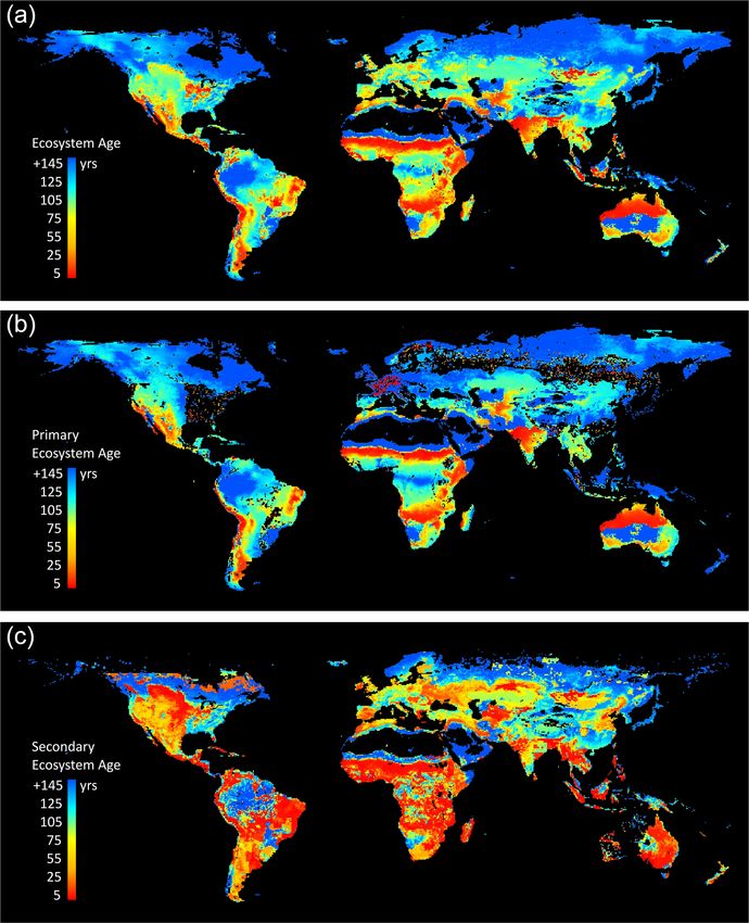
Abstract. Forest ecosystem processes follow classic re- (50–90◦ N) and younger tropical (23◦ S–23◦ N) ecosystems.
sponses with age, peaking production around canopy closure Between simulation years 1860 and 2016, land-use change
and declining thereafter. Although age dynamics might be and land management were responsible for a decrease in
more dominant in certain regions over others, demographic zonal age by −6 years in boreal and by −21 years in both
effects on net primary production (NPP) and heterotrophic temperate (23–50◦ N) and tropical latitudes, with the anthro-
respiration (Rh) are bound to exist. Yet, explicit represen- pogenic effect on zonal age distribution increasing over time.
tation of ecosystem demography is notably absent in many A statistical model helped to reduce LPJ-wsl v2.0 complex-
global ecosystem models. This is concerning because the ity by predicting per-grid-cell annual NPP and Rh fluxes
global community relies on these models to regularly up- by three terms: precipitation, temperature, and age class; at
date our collective understanding of the global carbon cy- global scales, R 2 was between 0.95 and 0.98. As determined
cle. This paper aims to present the technical developments by the statistical model, the demographic effect on ecosys-
of a computationally efficient approach for representing age- tem function was often less than 0.10 kg C m−2 yr−1 but as
class dynamics within a global ecosystem model, the Lund– high as 0.60 kg C m−2 yr−1 where the effect was greatest. In
Potsdam–Jena – Wald, Schnee, Landschaft version 2.0 (LPJ- the eastern forests of North America, the simulated demo-
wsl v2.0) dynamic global vegetation model and to determine graphic effect was of similar magnitude, or greater than, the
if explicit representation of demography influenced ecosys- effects of climate; simulated demographic effects were simi-
tem stocks and fluxes at global scales or at the level of a larly important in large regions of every vegetated continent.
grid cell. The modeled age classes are initially created by Simulated spatial datasets are provided for global ecosystem
simulated fire and prescribed wood harvesting or abandon- ages and the estimated coefficients for effects of precipita-
ment of managed land, otherwise aging naturally until an tion, temperature and demography on ecosystem function.
additional disturbance is simulated or prescribed. In this pa- The discussion focuses on our finding of an increasing role of
per, we show that the age module can capture classic demo- demography in the global carbon cycle, the effect of demog-
graphic patterns in stem density and tree height compared raphy on relaxation times (resilience) following a disturbance
to inventory data, and that simulated patterns of ecosystem event and its implications at global scales, and a finding of a
function follow classic responses with age. We also present 40 Pg C increase in biomass turnover when including age dy-
two scientific applications of the model to assess the mod- namics at global scales. Whereas time is the only mechanism
eled age-class distribution over time and to determine the that increases ecosystem age, any additional disturbance not
demographic effect on ecosystem fluxes relative to climate. explicitly modeled will decrease age. The LPJ-wsl v2.0 age
Simulations show that, between 1860 and 2016, zonal age module represents another step forward towards understand-
distribution on Earth was driven predominately by fire, caus- ing the role of demography in global ecosystems.
ing a 45- to 60-year difference in ages between older boreal
Published by Copernicus Publications on behalf of the European Geosciences Union.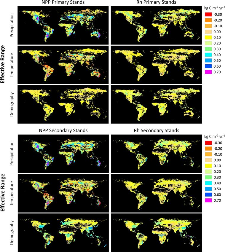
2576                                 L. Calle and B. Poulter: Age-class dynamics in LPJ-wsl v2.0 global ecosystem model

1   Introduction                                                  need the capability to represent landscape heterogeneity in
                                                                  forest structure and function.
Forest ecosystem production follows predictable patterns             Much of the evidence for the relative importance and
with time since disturbance. Classic forest age–production        global distribution of large disturbances has come from either
curves from Odum (1969) suggest that net ecosystem pro-           satellite retrievals of spectral indices indicating forest loss or
duction (NEP) peaks around canopy closure, declining there-       burn scars on the land (Potter et al., 2003; Frolking et al.,
after due to hydraulic limitations on gross primary produc-       2009; Pugh et al., 2019a), national forest inventory records
tion (GPP) (Ryan et al., 2004; Drake et al., 2010, 2011) and      of land-use change and forest management (Houghton, 1999;
increases in heterotrophic respiration from biomass turnover      FAO-FRA, 2015; Williams et al., 2016), or model-based
due stand-level declines in population density (Pretzsch          studies (Goldewijk, 2001; Arneth et al., 2017) that integrate
and Biber, 2005; Stephenson et al., 2014). That younger           information on historical land use (Goldewijk, 2001; Hurtt
forests are more productive than older forests has been long-     et al., 2006). Other natural disturbances such as pest and
standing knowledge in forestry, as evidenced by yield and         pathogen outbreaks, flooding, ice storms, and volcanic erup-
growth tables dating back to the 18th century that incorpo-       tions are less widespread globally (Frolking et al., 2009) but
rated stand age into their calculations of lumber production      are still influential drivers of landscape age-class dynamics
(Pretzsch et al., 2008).                                          (Dale et al., 2001; Turner, 2010). In the conterminous United
   On global scales, forest age is a considerable factor in the   States, forest management is the predominant forest distur-
global carbon cycle and comprises a large fraction of the total   bance (1.4 % of forested area converted to non-forest and
land carbon sink, which is estimated at 3.2±0.8 Pg C yr−1 for     then re-established annually), followed by fire (0.01 %–0.5 %
the years 2008–2017 (Le Quéré et al., 2018). According to         of forested area burned annually 1997–2008) (Williams et
country-level forest inventories, net carbon uptake from post-    al., 2016). Although pests and pathogens, namely bark bee-
disturbance tropical forest regrowth was 1.6 ± 0.5 Pg C yr−1      tle infestations, affected a much larger area (up to 6 % of to-
from 1990 to 2007 (Pan et al., 2011a). Although the time-         tal forested area in the US) than both logging and fire, their
frames for estimates of the total land sink and the inventory-    effects do not always cause immediate tree mortality. It is ar-
based regrowth flux do not perfectly overlap, the magnitude       guable whether fire and LUCLM are the two most important
of the regrowth sink relative to the total land sink warrants     global drivers of ecosystem age (Pan et al., 2011a), but never-
that models take regrowth dynamics into account. A multi-         theless these are the drivers applied in a model framework in
model global regrowth analysis with demographically en-           this study, in a manner that moves modeling one step forward
abled dynamic global vegetation models (DGVMs), to which          to assess global age-class dynamics.
Lund–Potsdam–Jena – Wald, Schnee, Landschaft version 2.0             The overall aims of this study are to present new model
(LPJ-wsl v2.0) contributed, estimated that post-disturbance       developments that simulate the time evolution of age-class
regrowth comprised a large global regrowth sink of 0.3 to         distributions in a global ecosystem model and to determine
1.1 Pg C yr−1 due to demography alone over the years 1981–        if explicit representation of demography in this model in-
2010 (Pugh et al., 2019b). In the last decade, explicit model     fluenced ecosystem stocks and fluxes at global scales or at
representation of forests as a function of time since distur-     the level of a grid cell. Technical details are presented for a
bance (hereafter simply, “ecosystem age”) has been a grand        module representing age-class dynamics, driven by fire feed-
challenge in an effort to quantify the demographic response       backs, land abandonment, and wood harvesting in the LPJ-
of forests to changes in climate, atmospheric CO2 , land-use      wsl v2.0 DGVM. Prior versions of LPJ-wsl v2.0 that in-
change and land management (LUCLM), and fire (Friend et           cluded early developments of the land-use change module
al., 2014; Kondo et al., 2018; Pugh et al., 2019b). Much of       and the age-class module have already contributed to previ-
the focus of these global modeling studies has been on the        ous studies (Arneth et al., 2017; Kondo et al., 2018; Pugh
effect of natural and anthropogenic disturbances on the car-      et al., 2019b). Analyses of model behavior, in terms of age–
bon dynamics in old-growth versus second-growth forests           structure and age–functional patterns, the temporal evolution
(Gitz and Ciais, 2003; Shevliakova et al., 2009; Kondo et         of age distributions and their causative drivers, and a statisti-
al., 2018; Yue et al., 2018; Pugh et al., 2019b) but lack finer   cal model of ecosystem production and respiration as a func-
distinction of demographic effects at different age classes.      tion of demography and climate, are presented.
Following a call to the science community to improve de-
mographic representation in models (Fisher et al., 2016),
there is now a growing list of global models that are ca-
pable of simulating global ecosystem demographics (Gitz
and Ciais, 2003, OSCAR; Shevliakova et al., 2009, LM3V;
Haverd et al., 2014, CABLE-POP; Lindeskog et al., 2013,
LPJ-GUESS; Yue et al., 2018, ORCHIDEE MICT; Nabel et
al., 2020, Jena Scheme for Biosphere Atmosphere Coupling
in Hamburg version 4 – JSBACH4), although more models

Geosci. Model Dev., 14, 2575–2601, 2021                                            https://doi.org/10.5194/gmd-14-2575-2021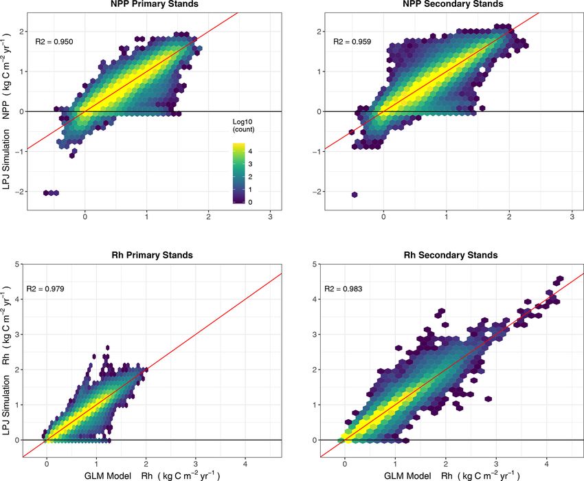
L. Calle and B. Poulter: Age-class dynamics in LPJ-wsl v2.0 global ecosystem model                                                  2577

                                                                         and soil texture are prescribed from driver datasets (Fig. 1).
                                                                         Vegetation is categorized into plant functional types (PFTs;
                                                                         Box, 1996). Plant populations compete for light, space, and
                                                                         soil water, depending on demand; nutrient cycles are not
                                                                         considered in this model version. LPJ-wsl v2.0 is a “big-
                                                                         leaf” ecosystem model, whereby leaf-level photosynthesis
                                                                         and respiration (Haxeltine and Prentice, 1996; Farquhar et
                                                                         al., 1980) occur at daily time steps, accounting for the photo-
                                                                         synthetically active period (daytime), and are scaled to the
                                                                         stand level using a mean-individual approximation, which
                                                                         assumes that important state variables (carbon stocks and
                                                                         fluxes) can be determined by using the average properties of a
                                                                         population. Plant populations are categorized using 10 PFTs
                                                                         in this study (phenology parameters and bioclimatic limits
                                                                         listed in Table S1), which are the same PFTs as in Sitch et
Figure 1. LPJ-wsl v2.0 model structure of inputs (red), time steps       al. (2003). Left unchanged are the PFT-specific bioclimatic
(blue), and the level at which state variables are tracked within grid   limits, turnover rates, C : N tissue ratios, allometric ratios,
cells and sub-grid-cell age classes (green), such as age classes or      and other parameters not explicitly commented on here but
land uses. Simulation of abiotic, biotic, and ecological processes       as described in Sitch et al. (2003). Mortality occurs as in the
occurs at the scale of an age class.                                     original version of LPJ, “. . . as a result of light competition,
                                                                         low growth efficiency, a negative annual carbon balance, heat
                                                                         stress, or when PFT bioclimatic limits are exceeded for a pe-
2     Methods                                                            riod of time” (Sitch et al., 2003). The fire module and the
                                                                         representation of land-use change and land management are
2.1     LPJ-wsl v2.0 general model description                           described in detail in Sect. 2.2.2, as these modules require
                                                                         a greater number of modifications for integration with age
2.1.1    LPJ history
                                                                         classes.
LPJ-wsl v2.0 has its legacy in the LPJ family of models,
first developed by Sitch et al. (2003) in a Fortran coding               2.2     Age-class module
environment1 . In 2007, Bondeau et al. (2007) produced the
LPJ managed Land (LPJmL) codebase, in C, which included                  2.2.1    An age-based model of ecosystems – sub-grid-cell
the addition of “managed lands”. The model known as LPJ-                          dynamics
wsl v2.0 is based on LPJmL v3.0 but includes modifications
                                                                         Age classes are represented as “patches” within a grid cell
to managed lands that now includes modeling gross land-
                                                                         (Fig. 1). Every age class has the same climate, atmospheric
cover transitions, forest age cohorts, and also a modification
                                                                         CO2 , and soil texture, but the properties of the age class, such
that include permafrost and wetland methane; the permafrost
                                                                         as available soil water and light availability, are determined
and wetland modules were not used in this study. Many de-
                                                                         by feedbacks from plant demand within an age class. Plant
velopments were made in the publicly available LPJmL4
                                                                         processes (competition, photosynthesis, respiration) are sim-
(version 4.0; Schaphoff et al., 2018) that are not present
                                                                         ulated at the level of the age class for each PFT within the
in LPJ-wsl v2.0. The LPJ-wsl v2.0 model was branched
                                                                         age class.
off of LPJmL some time around 2010 and continued to di-
                                                                            The age-class module has a fixed number of age classes
verge. This research paper represents a large effort toward
                                                                         that can be represented in a grid cell, but all age classes are
this end, and the LPJ-wsl v2.0 code is now freely and pub-
                                                                         not always represented. Age classes are classified into 12 age
licly available (https://github.com/benpoulter/LPJ-wsl_v2.0,
                                                                         classes in fixed age-width bins, defined as the unequalbin or
last access: 28 July 2020) under GNU Affero General Pub-
                                                                         the 10yr-equalbin age-width setup (Table 1). Each age class
lic License version 3.
                                                                         contains within-age-class elements, which are simply a vec-
2.1.2    LPJ-wsl v2.0 overview                                           tor representation of areas for each age unit in the age class.
                                                                         The within-age-class elements are not independent, and ev-
LPJ-wsl v2.0 simulates soil hydrology and vegetation dy-                 ery within-age-class element has the same state variables,
namics in 0.5◦ grid cells, wherein climate, atmospheric CO2 ,            including the same soil water and light. As such, we only
                                                                         simulate processes at the age-class level, and the within-age-
   1 LPJ and LPJmL history; https://www.pik-potsdam.de/research/         class elements are a simple method for a “smooth” transition
projects/activities/biosphere-water-modelling/lpjml/history-1 (last      between age classes. In theory, we can simulate processes
access: 28 July 2020).                                                   independently for each within-age-class element, but this is

https://doi.org/10.5194/gmd-14-2575-2021                                                   Geosci. Model Dev., 14, 2575–2601, 2021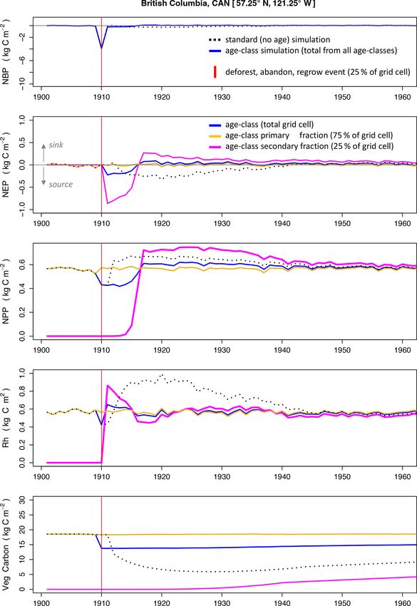
2578 L. Calle and B. Poulter: Age-class dynamics in LPJ-wsl v2.0 global ecosystem model
Table 1. Age-class widths corresponding to two different simulation managed land is abandoned and allowed to regrow – the frac-
age-class setups in LPJ-wsl v2.0. The age-class codes are referenced tional area undergoing an age transition is reclassified as a 1-
in figures. to 10-year age class. This process allows the model to accu-
rately track the carbon stocks, fluxes, and feedbacks associ-
Age widths (years) ated with these state variables. For example, if a fire burns
Code Unequal bins 10-year equal bins 50 % of an age class, then 50 % might have bare ground and
50 % will have vegetation at pre-burn levels. If the probabil-
1 1–2 1–10 ity of another fire is dependent on live vegetation, then feed-
2 3–4 11–20
backs will result in a lower chance of fire on the bare-ground
3 5–6 21–30
4 7–8 31–40
fraction versus the fully vegetated fraction that was not pre-
5 9–10 41–50 viously burned.
6 11–15 51–60 The most novel advancement in this study is a new method
7 16–20 61–70 of age-class transition modeling, which we call “vector track-
8 21–25 71–80 ing of fractional transitions” (VTFT), which improves the
9 26–50 81–90 computational efficiency of modeling age classes in global
10 51–75 91–100 models; there is a similar approach independently conceived
11 76–100 101–150 by Nabel et al. (2020). The method is a transparent and sim-
12 +101 +151 ple solution to the problem of dilution, which manifests as
an advective process when state variables, such as carbon
stocks or tree density, are made to merge by area-weighted
not practical or necessary. The main benefit for using equal- averaging. The concept of merging two unique age classes
bin or unequal-bin age classes is to independently simulate on the basis of similarity is a computational solution to con-
processes. The age widths of the age classes in the 10yr- strain the number of simulated age classes in accordance with
equalbin setup correspond to common age widths of classes computer resources but can be considered ecologically unre-
used in forest inventories; for contrast, JSBACH4 uses a 15- alistic. For example, along what axis of similarity is an age
year age width in their equal-bin age-class setup. Most age class considered to be most similar to another age class –
classes in this setup are represented by a vector of 10 ele- in terms of PFT composition, biomass in plant organs, plant
ments, wherein each element represents an aerial fraction for height, or stem density? Existing age-class models (Med-
each age unit (Table 1). The 10yr-equalbin age setup is used vigy et al., 2009, ED2; Lawrence et al., 2019, CLMv5.0; Yue
for all simulations including the global simulation, whereas et al., 2018, ORCHIDEE-MICT) employ merging rules (al-
the unequalbin setup is used for regional and single-grid-cell though some do not – Lindeskog et al., 2013, LPJ-GUESS)
simulations; simulation details are in next section. The use of with varying thresholds to ensure that age classes are only
equal or unequal age-class setups is more than just for report- merged if the difference among one state variable (biomass,
ing purposes. Resources available to plants (space, light, soil tree height) is less than a fixed threshold. We also merge age
water) differ between age classes but not within age classes, classes, but we do not employ merging rules along arbitrary
and we limit the model to represent a total of 12 age classes axes of similarity. We fix the number of age classes a priori,
only. Also, there exists a greater range of forest ages at global similar to LPJ-GUESS in that there is a maximum number
scales and the equal-bin age-class setup allows us to indepen- of age classes. Instead of forced merging to reduce computa-
dently model resource dynamics for more of the terrestrial tional burden (as in ED2), a fraction of the age class always
surface. If we had chosen the unequal-bin setup for global transitions to an older state, and a fractional area can tran-
simulations, we would be independently modeling processes sition and merge with the next oldest age class. By design,
only for the youngest age classes and we would lose capacity VTFT allows age classes to advance in a natural progression
to independently model processes at intermediate and older from young to old and ensures that age-class transitions al-
age classes. A study by Nabel et al. (2020), using the demo- ways occur between the most similar age classes along mul-
graphically enabled JSBACH4 DGVM, found that unequal tiple state variables.
binning of age widths had lower errors than equal-age-width The theoretical description of the VTFT approach is de-
binning but the largest reduction in model–observation error scribed as following in matrix notation. VTFT describes a
was achieved by simply adding more age classes at younger matrix of size (w indicates age widths per age class; n in-
ages, regardless of the binning strategy employed. dicates age classes), where the elements fi,j are the within-
Age classes are only created by disturbance, and we only age-class fractional areas of the grid cell:
model the following disturbances: fire, wood harvest, or land
f1,1 f1,2 . . . f1,n
abandonment, which initialize a new, youngest age class. The f2,1 f2,2 . . . f2,n
fraction of the age class that burns gets its age “reset” to the F= .
= fi,j ∈ R wxn .
(1)
. . .
.. .. .. ..
youngest age class (1–10 years). The same process occurs
for the fractional area that undergoes wood harvest or when fw,1 fw,2 ... fw,n
Geosci. Model Dev., 14, 2575–2601, 2021 https://doi.org/10.5194/gmd-14-2575-2021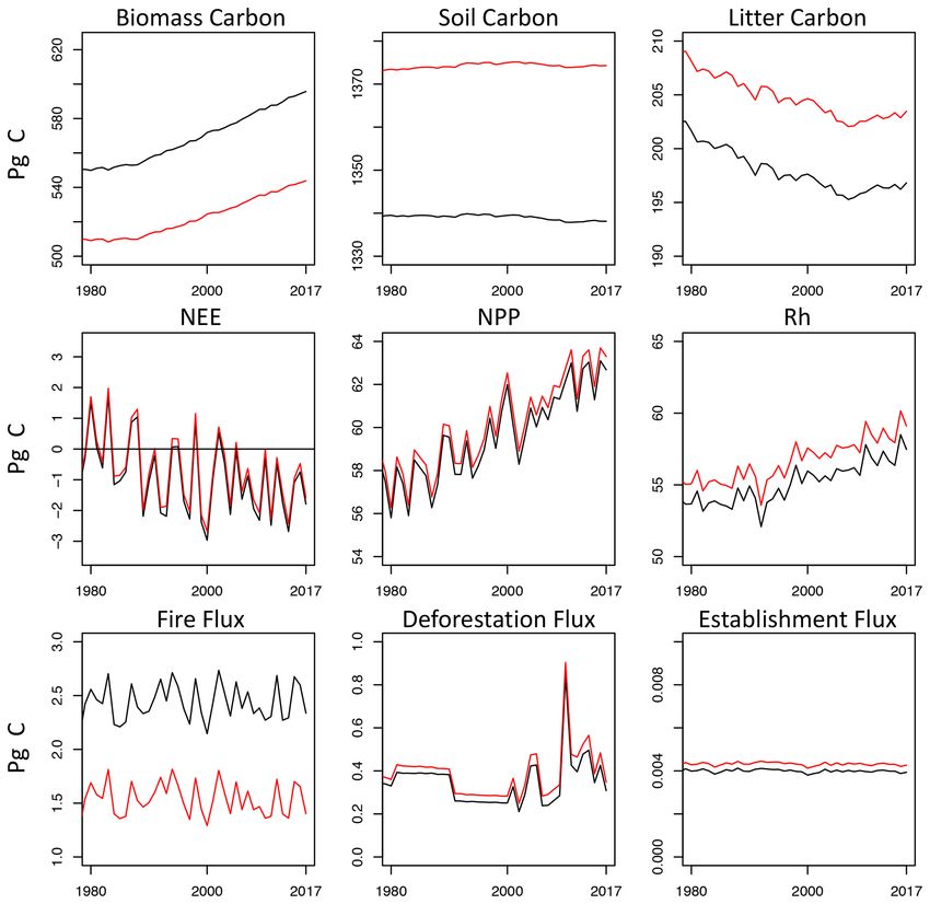
L. Calle and B. Poulter: Age-class dynamics in LPJ-wsl v2.0 global ecosystem model 2579
It is important to note here that within-age-class fractional the carbon remaining in the age class and the carbon in the
areas (fi,j ) are only used during age-class transitions – this transitioning fraction:
is a key point. For almost all calculations in LPJ, processes
(t) (t) (t) (t)
operate on the total fractional area for each age class: Cj × F 0 _totalj + Cj −1 × fw,j −1
(t+1)
Cj = (t) (t)
, (5)
F 0 _totalj + fw,j −1
Xn Xw
Ftotal = j =1
f
i=1 i,j
where F 0 _totalj is the total fractional area of age class (j )
Xw
F _totalj = f ,
i=1 i,j
(2) (t)
that remains in the age class, fw,j −1 is the transitioning or
where F _total is the sum of fractional areas for all grid-cell (t)
“incoming” fraction from the younger age class, and Cj −1 is
age classes, defined as the sum of fractional areas for over
age classes (n) and age widths (w). F _totalj is the column the carbon pool (on an area basis; kg m−2 ) in the younger
sum of F for a given age class (j ); the calculation can be age class, calculated at the end of the previous time step.
vectorized for efficiency by computing the dot product be- Equation (5) effectively converts the units of the carbon pools
tween an “all-ones” row vector of length (w) and F. In prac- from an area basis (km m−2 ) to a total mass (kg), taking the
tice, when LPJ-wsl v2.0 simulates physical processes on an sum of the carbon remaining and transitioning into the age
arbitrary carbon pool (C), for example, the calculations are class, and “redistributes” the carbon mass by the new frac-
computed on a per-mass basis, which then requires conver- tional area; during age-class transitions, these area-weighted
sion to a per-area basis by multiplying the total carbon mass averages are used to conserve mass across all state variables.
in an age class by the representative total fractional area: In theory, VTFT minimizes the redistribution (or “dilution”)
h i of mass across a larger area if the incoming fractional area
Cj kg m−2 = Cj kg × F _totalj ,
(3) is much smaller than the fractional area of the existing age
class.
In a plain-language summary of the matrix representation,
where Cj (units: kg or km−2 ) is the total carbon for a given
VTFT ensures that a vector of fractional areas is associated
age class (j ). Again, the calculation can be computed via
with every age class (n), of length (w), and where “w” is
the Hadamard (element-wise) product, taking a vector (C),
equal to the age width of the age class, with elements (f )
where elements are the carbon pool totals for every age class
that are the fractional areas contributing to the total fractional
and multiplying by vector F _total, with elements of the to-
area of the age class (F _total). When a young age class (a1 )
tal fractional areas in each age class. In effect, all simulated
is first created, VTFT vectors are initialized to zero and the
processes in LPJ-wsl v2.0 act on an area basis, based on the
first element (f1 ) is set to the incoming fractional area. The
column sums of F.
following is a description for within-class and between-class
In every year of simulation, an age-class transition always
transitions.
occurs, and this procedure is defined as an operation that in-
Within-class fractional transitions. For every simulation
crements the positions of the elements as
year, the position of each element (fx ) in the VTFT vector is
F(t+1) := incremented by the representative time of each element (x),
(t+1) def (t+1) (t+1) def (t) (t+1) def (t) which is simply 1. No changes occur to the state variables of
f1,1 = fnew f1,2 = fw,1 ... f1,n = fw,n−1
(t+1) def (t) (t+1) def (t) (t+1) def (t) the age class during within-class transitions.
f2,1 = f1,1 f2,2 = f1,2 ... f2,n = f1,n
Between-class fractional transitions. Upon incrementing
,
. . .. .
. . .
. . . .
the position of each element in the VTFT vector, if the value
(t+1) def (t) (t+1) def (t) (t+1) def (t) (t) at fw is non-zero, then the corresponding fractional area fw ,
fw,1 = fw−1,1 fw,2 = fw−1,2 ... fw,n = fw,n + fw−1,n
(4) defined as the outgoing fraction, is used in an area-weighted
average between the state variables of a1 fw and the next old-
where the superscripts are the time indices for the current est age class a2 F _total. Upon incrementing the element po-
time step (t + 1) and the previous time step (t), subscripts are sition, if all elements in the VTFT vector of the preceding
(t+1)
the matrix indices, fnew is the fractional area of a newly age class are zeros then the age class is simply deleted from
created stand (by definition, it is the youngest age-class frac- computational memory.
tion), and fw,n is the oldest fractional age of the grid cell, Two hypothetical scenarios are provided in Fig. 2 that
which is incremented by an amount equal to fractional area demonstrate age-class transitions using the VTFT procedure
(t)
(fw−1,n ). Of special importance is the bottom row of the F when there is a young age class created, and when there
matrix, Fw,1≤j ≤n , which includes the fractional areas of each are fractional age-class transitions between age classes. With
age class transitioning to the next-oldest age class. The tran- VTFT, any number of age classes and age widths can be
sitioning fractions (Fw∗ ) become the incoming fractions in modeled, but it is demonstrated in this study that the age
the next-oldest age class. Using an arbitrary carbon pool (C) widths employed in this study are sufficient to minimize the
as an example, the carbon pool for the next time step (t + 1) dilution of state variables when area-weighted averaging is
would be calculated via an area-weighted average between used to merge fractional age classes while also simulating
https://doi.org/10.5194/gmd-14-2575-2021 Geosci. Model Dev., 14, 2575–2601, 2021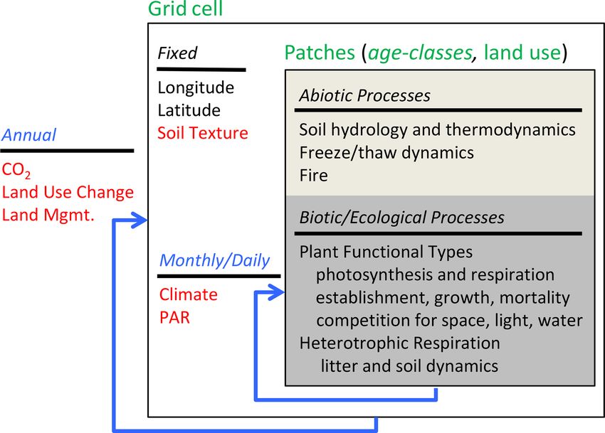
2580                                    L. Calle and B. Poulter: Age-class dynamics in LPJ-wsl v2.0 global ecosystem model

Figure 2. Methodological examples of the matrix-based method called vector-tracking of fractional transitions for computationally efficient
simulation of age classes in large-scale models. (a) Hypothetical matrix of VTFT vectors of fractional areas (f ). The total area of the age
class is the sum of the fractional areas in the corresponding VTFT vector. State variables are calculated on an area basis by accounting for
the fractional area of the age class; in this example, Csoil is the carbon in soil. (b) An example of the VTFT method for a newly created age
class by clear-cut wood harvest. An area-weighted average updates age-class state variables in the youngest age class using the preceding
total fractional area of the age class and the incoming fraction. (c) A VTFT example for a fractional age-class transition. An area-weighted
average updates state variables in an age class using the preceding total fractional area of the age class and the incoming fraction from the
younger age class.

stand–age patterns in state variables of carbon stocks, stem             litter in the age class, gets calculated as an immediate flux to
density and fluxes.                                                      the atmosphere. The fraction of the PFT population that does
                                                                         not burn maintains state variables (e.g., tree height, carbon
2.2.2   Integration with fire and LUCLM modules                          in leaf and wood) at previous values. It is possible to have
                                                                         so-called “survivor” trees on the youngest age class that then
The disturbance processes of simulated fire, land-use change,            skew the age-height distribution of the age class. The model
and land management can occur on multiple age classes at a               does not assume any structure of survivor trees. Instead, sur-
time. That is, these processes are related but independent.              vivor trees occur as a function of the underlying process. For
For instance, fire can occur independently on each age class,            example, if a fire occurs on a stand, but the fire does not burn
and each age class would have its own independent esti-                  all the PFTs, then there will be survivor PFTs on the stand.
mate of the probability of fire. Wood harvest occurs first on            Both fire and wood harvest (below) are simulated based on
the oldest age class and progressively harvests younger age              fractional area, and it is the fractional area, specifically, that
classes until two demands are met (harvest area and harvest              gets reset to a young age class.
biomass), described in detail in the relevant section below.                 LUCLM. Age classes get created when managed land (i.e.,
Clearly, each process influences the other as logging or fire            crop and/or pasture) is abandoned and allowed to regrow into
both remove biomass that could be potential fuel for a fu-               secondary forests, or when wood harvest occurs on forested
ture fire or biomass for a future harvest. These relationships           lands and causes deforestation. In both cases, the fractional
are not evaluated here but are noted for their potential impor-          area abandoned or logged initiates the creation of a youngest
tance. Below, we describe in detail the integration of the age-          age class, or it gets merged with a youngest age class if one
class module with the two prominent forms of disturbance:                exists already. To improve the account of primary forests, de-
fire and LUCLM.                                                          fined here as natural land without a history of LUCLM, and
   Fire. The fractional area burned initiates the creation of a          second-growth forests, defined as natural land with a history
youngest age class, or it gets merged with a youngest age                of LUCLM, transitions between these classes are unidirec-
class if one exists already. Fire simulation is based on the             tional from primary to secondary. In the LUCLM module,
semi-empirical Glob-FIRM model by Thonicke et al. (2001),                gross transitions between land uses are simulated (Pongratz
with implementation details described in Sitch et al. (2003).            et al., 2014; Stocker et al., 2014), such that if the fraction
In short, fire is dependent on the length of the fire season, cal-       of abandoned land equals the fraction of land deforested in
culated as the number of dry days in a year above a threshold            the same year (net zero land-use change), then the fluxes
and a minimum fuel load, defined only as the mass of carbon              from the gross transitions are tracked independently and give
in litter. When a fire occurs, PFT-specific fire resistances de-         an overall more accurate account (and higher magnitude) of
termine the fraction of the PFT population that gets burned.
The biomass of burned PFTs, along with the aboveground

Geosci. Model Dev., 14, 2575–2601, 2021                                                    https://doi.org/10.5194/gmd-14-2575-2021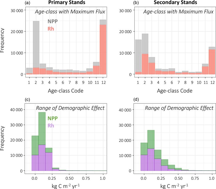
L. Calle and B. Poulter: Age-class dynamics in LPJ-wsl v2.0 global ecosystem model                                        2581

emissions from LUC than if we only tracked net transitions       2.3     Experimental design and analysis
(Arneth et al., 2017).
   General rules distinguishing primary and secondary stands     2.3.1    Model inputs
within the age-class context stem from the Land Use Harmo-
nization dataset version 2 (LUHv2; Hurtt et al., 2020) but       Inputs to the model are gridded soil texture (sand, silt,
with the following modifications so that the LUHv2 data can      clay fractions) from the USDA Harmonized World Soils
be used in LPJ-wsl v2.0. (1a) The primary grid cell fraction     Dataset v1.2 (Nachtergaele et al., 2008), annually varying
only decreases in size and never gets mixed with existing sec-   global mean [CO2 ] (time series available in the Supplement),
ondary forests or with abandoned managed land. Only fire         and monthly varying air temperature, precipitation, precipi-
creates young age classes on primary lands. (2a) Secondary       tation frequency, and radiation from the Climate Research
grid cell fractions can be mixed with other secondary for-       Unit (CRU, version TS3.26) data for 1901–2016. Land use,
est fractions, recently abandoned land, fractions with wood      land-use change, and wood harvest were prescribed annu-
harvest, and recently burned area. General priority rules for    ally based on LUHv2 (Hurtt et al., 2020), which is used as
deforestation and wood harvest. (1b) For simplicity, defor-      forcing land use for the sixth Coupled Model Intercompar-
estation (i.e., land-use change) always occurs in the rank-      ison Project (CMIP6; Eyring et al., 2016). The dataset in-
ing of oldest to youngest age class, proceeding to deforest      cludes fractional area of bi-directional (gross) land-use tran-
each age class until the prescribed fractional area of defor-    sitions between forested and managed lands, as well as the
estation is met. This rule will always result in greater land-   total biomass of wood harvest on a specified fractional area
to-atmosphere fluxes than if rules were employed that al-        logged. In LPJ-wsl v2.0, managed lands (i.e., crop and/or
lowed younger age classes to be preferentially deforested.       pasture) are treated as grasslands with no irrigation, no fire,
(2b) Wood harvest (i.e., biomass harvest) also occurs in the     and tree PFTs were not allowed to establish. Model represen-
ranking of oldest to youngest age class until two conditions     tation of land management is an oversimplification to focus
are met. Timber harvest occurs on each age class until a pre-    on effects of wood harvest.
scribed harvest mass or harvest area is met.
   Treatment of immediate emissions and residues. Defor-         2.3.2    Examining age dynamics: qualitative evaluation
estation results in 100 % of heartwood biomass and 50 % of                of regional simulations against the US Forest
sapwood biomass being stored for delay emission in prod-                  Inventory Analysis data to assess simulated
uct pools; root biomass is entirely part of belowground litter            changes in stand structure and ecosystem
pools, while 100 % leaf and 50 % of sapwood biomass be-                   function
comes part of aboveground litter pools. Grid cell fractions
that underwent land-use change were not mixed with ex-           US Forest Inventory and Analysis (FIA). The FIA dataset
isting managed lands or secondary fractions until all land-      is freely available at the FIA DataMart web portal (FIADB
use transitions had occurred. This avoids a computational se-    version 1.6.0.0.2), accessed 2 February 2016. The FIA plot-
quence that results in a lower flux if deforestation and aban-   level data are composed of four circular subplot sample ar-
donment occur in the same year. For wood harvest, 100 % of       eas (168 m2 ), wherein attributes of all trees with diame-
leaf biomass and 40 % of the sapwood and heartwood enters        ter at breast height (DBH) ≥ 5.0 in (12.7 cm) diameter are
the aboveground litter pools, and 100 % of root biomass the      recorded. We extracted variables that capture two main axes
belowground litter pools; 60 % of sapwood and heartwood          of structural change as a function of forest age: stem den-
are assumed to go into a product pool for delayed emission.      sity and tree height. Spatial coordinates of sample plots are
   Timber from deforestation and harvest in product pools        “fuzzed” with imposed error for privacy reasons (FIA User
for delayed emission (Earles et al., 2012). For deforestation,   Guide v 6.02; O’Connell et al., 2015). For purposes of this
60 % of exported wood (i.e., not in litter) goes into a 2-year   analysis, plot data were aggregated to the spatial scale of the
product pool, and 40 % goes into a 25-year product pool, fol-    US Forest Service Divisions (Fig. S2; USFS Divisions are
lowing the 40 : 60 efficiency assumption from McGuire et         delineated by regional-scale precipitation levels and patterns
al. (2001). For wood harvest, the model uses space–time ex-      as well as temperature) minimizing co-location concerns be-
plicit data on harvest fractions going into roundwood, fuel-     tween model–observation comparisons. We filtered the FIA
wood, and biofuel product pools. We use three product pools      data based on the following criteria. We only included plots
and assume that 100 % of the fuelwood and biofuel fraction       that used the national standard plot design (DESIGNCD of
goes into the 1-year product pool (emitted in the same year      1) and were located on forested land (COND_STATUS of
of wood harvest), 50 % of the roundwood fraction goes into       1) with no history of major disturbance, stocking, or logging
the 10-year product pool (emitted at rate 10 % per year), and    (DSTRBCD of 0; TRTCD1 of 0), which could alter natural
the remaining 50 % of the roundwood fraction goes into the       patterns of tree density versus age and confound the compar-
100-year product pool (emitted at rate 1 % per year).            ison to simulated data. We also only included plots that had
                                                                 both subplot samples of live tree (STATUSCD of 1) stem
                                                                 density and also circular micro-plot (13.5 m2 ) stem density

https://doi.org/10.5194/gmd-14-2575-2021                                           Geosci. Model Dev., 14, 2575–2601, 2021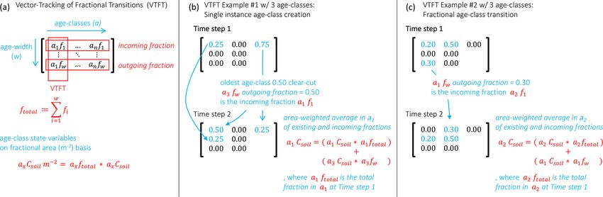
2582                                 L. Calle and B. Poulter: Age-class dynamics in LPJ-wsl v2.0 global ecosystem model

samples of seedlings and/or saplings (defined as trees 1 to       2.3.3   Examining resilience: idealized simulation of a
5 in (2.54 to 12.7 cm) in diameter), and where the subplot                single event of deforestation, abandonment, and
sampling design was the national standard (tree table SUBP                regrowth
of [1,4]); LPJ-wsl v2.0 implicitly includes sapling and adult
trees in estimates of tree height and stem density. We as-        The objective of the idealized simulation was to evaluate the
sumed that the filtered plots were representative of the true     effect of age classes on relaxation times following a sin-
density and distribution of tree species for the general vicin-   gle deforestation, abandonment and regrowth event within
ity of the plots and of the USFS Division. Although these         a single grid cell (Table 2). The relaxation time is defined
requirements for selecting FIA plots reduce the total amount      as the time required for a variable to recover to previous
of data, we aimed to make evaluations in a fair manner, in        state and is a direct measure of ecosystem resilience (sensu
both spatial scale and meaning.                                   Pimm, 1984). Two simulations were conducted, the first sim-
   Regional simulations. The objectives of the regional simu-     ulation used the 10-yr-equalbin age-width setup, Sage_event ,
lations (Table 2) were to evaluate demographic patterns of        and another did not simulate age classes, Snoage_event (Ta-
stand structure and function when simulating age classes          ble 2). Both simulations were conducted with a 1000-year
using different age-width binning. Two idealized simula-          “spinup” using fixed CO2 (287 ppm, pre-industrial value)
tions were conducted at a regional scale to sample simu-          and climate randomly sampled from 1901–1920 to ensure
lated annual stem density, average tree height, and NEP.          that state variables were in dynamic equilibrium. A tran-
The first simulation used the unequalbin age-width setup,         sient simulation then used time-varying CO2 and climate,
Sunequalbin , and another used the 10-yr-equalbin age-width       as prescribed by model inputs. Fire and LUCLM were not
setup, S10 yr bin (Table 2). For both simulations, fire and LU-   simulated. Instead, 25 % of the fractional area was defor-
CLM were not simulated. Instead, 5 % of the fractional area       ested in year 1910 of the simulation and classified as man-
of age classes > 25 years were cleared of biomass annually;       aged land. Treatment of deforestation byproducts (i.e., car-
the fractional area cleared was reclassified and merged with      bon in dead wood left on site) were the same in both simula-
the youngest age class. The intent of the setup was to ensure     tions. In the following year (1911), the managed land fraction
that each grid cell maintained fractional area in every age       was abandoned and allowed to regrow. The following state
class for each year of the simulation and avoided situations in   variables were plotted over time and visually evaluated: net
which age classes were only present in “bad years”, or when       biome production (NBP, defined as the difference between
growing conditions were poor. Both simulations were con-          NEP and LUC_flux), NEP, net primary production (NPP),
ducted with a 1000-year “spinup” using fixed CO2 (287 ppm,        heterotrophic respiration (Rh), and carbon in biomass.
“pre-industrial” values) and climate randomly sampled from           The idealized simulations were performed for a single
1901–1920 to ensure that age distributions were developed         grid cell in a mixed broadleaf and evergreen needleleaf
and state variables were in dynamic equilibrium (i.e., no         forest in British Columbia, Canada (57.25◦ N, 121.25◦ W).
trend). A transient simulation then used time-varying CO2         The grid cell is a boreal climate with total annual rain-
and climate, as prescribed by model inputs. Stand structure       fall 473.7 mm yr−1 (average over 1980–2016, based on CRU
data were analyzed for 1980–2016.                                 TS3.26) with monthly minimum 9.11 mm per month and
   The idealized simulations were performed for the mixed         maximum of 105.8 mm per month. Mean annual tempera-
deciduous and evergreen forests of Michigan, Minnesota,           ture (1980–2016, CRU TS3.26) was 0.59 ◦ C with a monthly
and Wisconsin in the US (bounding box defined by left:            minimum of −16.9 ◦ C and maximum 14.7 ◦ C.
97.00◦ W; right: 82.50◦ W, top: 49.50◦ N, bottom: 42.00◦ W).
These forests are of moderate temperate climates, with            2.3.4   Global simulation objectives and setup
total annual rainfall 815.0 mm yr−1 (average over 1980–
2016, based on CRU TS3.26), a time-series minimum of              There were three main objectives for global simulations. The
21.0 mm per month, and a maximum of 148.5 mm per month.           first objective was to evaluate the contribution of age-class
Mean annual temperature (1980–2016, CRU TS3.26) was               information to global stocks and fluxes. Here, a simulation
5.98 ◦ C with monthly minimum of −11.45 ◦ C and maximum           with age classes (Sage ) was compared to a simulation without
20.98 ◦ C.                                                        age-class representation (Snoage ) (Table 2). The second objec-
   Data were pooled for the region over the time period and       tive was to determine the relative influence of fire and LU-
by age class. Data were plotted in boxplots to show median        CLM on the spatial and temporal distribution of ecosystem
value, interquartile range, and outliers. No attempt was made     ages. For this objective, a fire-only simulation (SFire ) had age
to detrend data because there was enough between-age-class        classes only created by fire, whereas a LUCLM-only simu-
variation to evaluate general demographic patterns visually.      lation (SLU ) had age classes only created by abandonment
                                                                  of managed land or by wood harvest (Table 2). A simula-
                                                                  tion with both fire and LUCLM (SFireLU ) was used as the
                                                                  baseline for comparison against SFire and SLU . The third and
                                                                  fourth objectives used data from Sage (Sage = SFireLU ) to de-

Geosci. Model Dev., 14, 2575–2601, 2021                                            https://doi.org/10.5194/gmd-14-2575-2021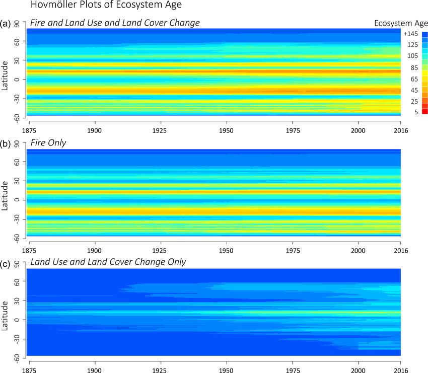
L. Calle and B. Poulter: Age-class dynamics in LPJ-wsl v2.0 global ecosystem model                                                                                  2583

Table 2. Description of LPJ-wsl v2.0 simulations in this study, corresponding objectives and related science questions.

  Simulation            Description                                            Objective and questions                                 Structure/processes included
                                                                                                                                     Age classes        Fire   LUCLM
  Single cell
  Sage_event            Idealized simulations of a defor-                      Evaluate recovery dynamics of a single                      X              X     X
                        est, abandon, and regrow event in                      regrow event. Do age dynamics influ-
                        British Columbia, Canada (57.25◦ N,                    ence relaxation times?
  Snoage_event          121.25◦ W)                                                                                                         ×              X     X
  Regional
   a
  Sunequalbin           Idealized simulation with 5 % of                       Does the model capture “classic” demo-                      Xa             ×     ×
                        grid cell cleared annually to create a                 graphic patterns in stand structure (tree
                        wide age-class distribution in mixed                   density and height) and function (NEP,
                        broadleaf and evergreen temperate                      NPP, Rh)?
                        forests of Michigan (MI), Minnesota,
   b
  S10yrbin                                                                                                                                 Xb             ×     ×
                        and Wisconsin (WI) in the US
  Global
  Snoage                Standard-forcing factorial simulations                 Do age dynamics influence global                            ×              X     X
                        at global scale                                        stocks and fluxes?
  SFire                                                                        What is the relative contribution of fire                   X              X     ×
                                                                               and LU to ecosystem age?
  SLU                                                                          Are demographic effects evident in                          X              ×     X
                                                                               fluxes, and where is the effect greatest?
  SFireLU (Sage )                                                              What is the relative contribution of cli-                   X              X     X
                                                                               mate versus demography on fluxes?
a Unequal age-width simulation. Age widths are as described in Table 1. b The 10-year interval age-width simulation. Age widths are as described in Table 1.

termine where the effect of demography was greatest and to                                 SFireLU . The first assessment was made by visual inspection
identify the relative influence of demography versus climate                               of zonally averaged time series (i.e., Hovmöller plots) for the
on simulated fluxes (NEP, NPP, and Rh).                                                    entire period of transient simulation (1860–2016). In addi-
   For all global simulations, a spinup simulation was run                                 tion, for each of SFire and SFireLU , a simple linear regres-
for 1000 years using randomly sampled climate conditions                                   sion model (age is equivalent to β0 + β1 · year, setting 1860
from 1901–1920 and atmospheric CO2 fixed at pre-industrial                                 as the reference year and defined as 1) was applied to iden-
levels (287 ppm) and no land use or wood harvest; spinup                                   tify trends in ecosystem age by the following zonal bands:
ensured that age distributions and state variables were in                                 boreal (50 to 90◦ N), temperate (23 to 50◦ N), and tropics
dynamic equilibrium (i.e., no trend). For simulations with                                 (23◦ S to 23◦ N). Trends in age distributions due to LUCLM
land use, a second “land-use-spinup” procedure was run for                                 are not prescribed by inputs per se; instead, the age module is
398 years to initialize land-use fractions of crop and/or pas-                             a necessary model structure that allows full realization of the
ture to year 1860, resampling climate and fixing CO2 as in                                 effect of forcing data on age distributions. Trends in age dis-
the first spinup. After spinup procedures, climate and CO2                                 tribution due to fire, which is a simulated process as opposed
were allowed to vary until simulation year 2016; in SLU and                                to prescribed, result from climate and fuel load feedbacks on
SFireLU , land-use change and wood harvest varied annually                                 fire simulation.
as prescribed by the LUHv2 dataset.
   In the first objective (as above), global values for stocks
and fluxes include both natural and managed lands. These                                   2.3.5     Statistical model to assess relative importance of
global estimates conform to typical presentation of global                                           demography and climate
values (Le Quéré et al., 2018), in petagrams (1015 ) of car-
bon. Comparisons are made among simulation types and to
values from the literature.                                                                For the third objective of global simulations – to reduce di-
   For the second objective, a time series of zonal mean                                   mensionality of the data and to assess the relative influence
ecosystem ages were analyzed to determine the relative im-                                 of demography and climate on simulated fluxes – annual flux
portance of SFire and SLU on the observed distributions in                                 data from Sage (Table 2) were analyzed from 2000–2016 us-

https://doi.org/10.5194/gmd-14-2575-2021                                                                            Geosci. Model Dev., 14, 2575–2601, 2021
2584                                      L. Calle and B. Poulter: Age-class dynamics in LPJ-wsl v2.0 global ecosystem model

ing a generalized linear regression model:                            3     Results

fluxi,yr = B1i × total_precipitationi,yr                              3.1     Model stand structure – comparison against
        + B2i × mean_temperaturei,yr                                          inventory data
        + B3i,ageclass × ageclassi,yr ,                        (6)    FIA data were not equally available for every age class, nor
                                                                      for every division (Fig. S2), but there were enough inven-
where “flux” was either NEP, NPP, or Rh in kg C m−2 yr−1 ,            tory data across eight divisions, spanning subtropical to tem-
precipitation (mm) and temperature (Celsius) data from CRU            perate steppe climates, to qualitatively suggest that LPJ-wsl
TS3.26, and “ageclass” was categorical, defined by the age-           v2.0 does capture the expected patterns of tree density and
class code (Table 1), and the beta coefficients (B) for sub-          height per age in the different climates evaluated. There was
scripts of grid cells (i), years (yr), and age class. The beta        a tendency for LPJ-wsl v2.0 to overestimate stem density in
coefficients are therefore unique to every grid cell, and the         younger age classes and systematically underestimate tree
betas for age classes are estimated separately for each age           heights among age classes (e.g., Figs. S3, S5), for which the
class within the grid cell (B3i,age ). An initial test of the model   greater number of small individuals could cause the average
attempted to estimate globally consistent predictor effects,          tree heights to be dampened. However, LPJ-wsl v2.0 is a big-
but the model was found to be a poor fit (not shown) and it           leaf, single-canopy model that include space-filling “pack-
was assumed that there was too much variation among grid              ing” constraints on stem density, based on allometric rules
cells to detect globally consistent effects. Instead of adding        for size and height of PFTs. Also the model does not repre-
additional gridded fields of predictor variables to account for       sent multiple PFT cohorts in an age class, or more simply, it
grid-cell-level variation, the same statistical model was ap-         does not represent vertical heterogeneity such as understory
plied and analyzed per grid cell. This allowed coefficients of        growth that would otherwise increase stem density. As such,
precipitation, temperature and “ageclass” to vary by grid cell,       and under the current model architecture and associated as-
in essence, reducing the effect of variation in PFT composi-          sumptions, the exact cause of the mismatch is unclear. Even
tion, soil texture, and hydrology that might otherwise reduce         still, the more general pattern of modeled stem density and
predictive power.                                                     tree height tended to track FIA data, with stem density being
   In all grid cell analyses, the intercept term was intention-       maximal in the younger age classes and declining thereafter,
ally omitted from the data model by adding a “−1” term to             whereas tree height patterns increased more linearly before
the data model. The “ageclass” term in the statistical model          stabilizing (Figs. S6 to S9).
(B3i,age ), as a categorical variable, effectively takes the place       FIA data had greater variability among age classes, regard-
of the intercept term anyhow, so the outcome is that esti-            less of division. FIA data are not aggregated by PFT, instead
mates are for the absolute effect of each age class on the            they are species-level data. Changes in species composition
predicted flux as opposed to estimates that were relative             over time do occur and can add to the observed variability
to the first age class; this had no impact on estimated co-           among age classes in tree density and tree height. LPJ-wsl
efficients but it did simplify analyses. In grid cells where          v2.0 includes a limited set of PFTs, which most likely lim-
only a single age class was present, the statistical model            its the model’s capacity to represent similar levels of vari-
was defined as (fluxi,yr = B1i total_precipitationi,yr + B2i          ation in tree density and tree height. It is beyond the scope
mean_temperaturei,yr + B3i ), leaving the intercept term, in          of this study to disentangle these patterns further, but greater
this case – B3i , to be estimated from the data and then re-          agreement between observed and simulated patterns of for-
classifying the intercept term by the age-class code for the          est structure might be achieved by including additional plant
grid cell.                                                            functional types that are representative of tree species for a
   The degrees of freedom (DoFs) of a model for a grid cell           given division.
with a single age class was 14 DoFs, based on 17 annual
data points to estimate coefficients of three predictors. The         3.2     Model age dynamics
degrees of freedom for a grid cell that had a maximum of 12
age classes was 190 DoFs, based on 204 annual data points to          3.2.1    Dynamics of stand structure and function –
estimate coefficients for 14 predictors. Because the analysis                  regional simulations
produced statistical results for every grid cell, the degrees of
freedom are not presented elsewhere. Coefficients were only           Forest structural characteristics of stem density, height, and
analyzed or mapped when significant at p = 0.05.                      NEP followed the expected patterns with age with a few ex-
                                                                      ceptions. In Sunequalbin (Table 2), stem density increased from
                                                                      near zero to maximum in the 21- to 25-year age class, before
                                                                      declining non-linearly (Fig. 3). By contrast, the gradual in-
                                                                      crease in stem density in the first age class in S10−yrbin (Ta-
                                                                      ble 1) was not readily apparent because this process, which

Geosci. Model Dev., 14, 2575–2601, 2021                                                https://doi.org/10.5194/gmd-14-2575-2021
L. Calle and B. Poulter: Age-class dynamics in LPJ-wsl v2.0 global ecosystem model 2585
is evident in Sunequalbin , occurs entirely within the youngest tern is reflective of simulated model dynamics. This emer-
1- to 10-year age class in S10−yrbin . Both simulation setups gent pattern could lend itself to observational constraints if
approach the same stem densities after age ∼ 25; prior dif- similar emergent patterns can be derived from forest inven-
ferences are due to binning of age widths. tory data in the future.
For average tree height in Sunequalbin , there were large tree
heights in the youngest age class, which results from so-
3.2.2 Time-series evolution of a deforestation,
called “survivor” trees (Fig. 3). Not all trees are killed off
abandonment, and regrow event
when a disturbance occurs in LPJ. Although the age class is
“reset” to the youngest age class, the survivor trees skew the
height distribution until the density of establishing saplings A single event of deforestation, abandonment, and subse-
subsequently increases and brings down the average tree quent forest regrowth caused long-lasting effects on carbon
height to smaller values. This pattern is more akin to what balance and dynamics when omitting age-class dynamics.
occurs during natural fires or selective harvesting, which can In the simulation without age classes, Snoage_event (Table 2),
reduce the overall age but might not result in a complete re- grid-cell-level NEP takes ∼ 30 years to recover to values
moval of all trees. By contrast, the skewed age-height pattern prior the event, whereas the age-class simulation, Sage_event ,
is not apparent in S10−yrbin (Fig. 3) only because the same takes only 5–6 years to recover (Fig. 5) – a 5-fold change in
process is effectively hidden. Both simulation types approach relaxation times. The quick recovery of grid-cell-level NEP
the same average tree heights after age ∼ 25 (Fig. 3). in Sage_event is due partly to the fact that the fraction of the
NEP peaked at age classes 5–6 in Sunequalbin , before declin- grid cell (75 %) that was not deforested maintained its state
ing non-linearly to the lowest average value in the oldest age variables (carbon stocks in vegetation, soil, litter) unchanged
class (Fig. 3). Although the unimodal peak was not apparent from its prior state, which buffered NEP and dampened the
in S10−yrbin , the maximum NEP occurred in the youngest age effect of the smaller fraction (25 % of grid cell) that was
class and also declined non-linearly thereafter (Fig. 3). The deforested. Age-class dynamics also contributed an elevated
decline in NEP after a maximum at 5–6 years was driven NEP (Fig. 5) that quickens the recovery at the grid cell level.
mainly by an increase in Rh due to increases in turnover In Sage_event , there is an elevated NEP in the secondary stand
rather than a larger decline in NPP (Fig. 4). The peak in NEP that is sustained for more than 30 years following the event.
did not coincide with maximum tree density at ∼ 20 years. In Snoage_event , vegetation dynamics cause turnover to in-
Instead, model dynamics suggest that the total foliar projec- crease and cause an elevated grid-cell-level Rh that is con-
tive cover of tree canopies reaches near maximum (80 %– sistently higher than grid-cell-level NPP for 30 years af-
95 % cover; not shown) at 5–6 years, thereafter plant compe- ter the event. This pattern is striking because NPP recovers
tition reduces NPP while biomass turnover increases, which quicker than in Sage_event and maintains an elevated value for
together cause the apparent decline in NEP. The time period ∼ 30 years. Following a disturbance event in LPJ, stem den-
of canopy closure, at 5–6 years, in LPJ-wsl v2.0 is probably sity and foliar projective cover is reduced but the state vari-
too early, in part due to advanced regeneration (saplings es- ables (carbon in plant organ pools of leaf, stem, root) main-
tablish at 1.5 m height) and constant establishment rates. The tain prior values; this is the reason grid-cell-level NPP re-
age-class module qualitatively demonstrates NEP–age rela- covers quickly in the standard no-age simulation. As stand
tionships consistent with field-based evidence (Ryan et al., density increases again, canopy closure initiates competitive
2004; Turner, 2010). dynamics that result in mortality of individuals of the plant
Lastly, an emergent pattern was found in the declining por- population that are generally larger than if the stand had pro-
tion of the NEP–age curve and approximately follows the gressed from small to large individuals (as in Sage_event ).
functional form NEPmax · 0.70age−agemax , where “NEPmax” The VTFT module also uses the mean-individual approx-
is the maximum NEP flux at the initial point of decline, imation but stand dynamics are always allowed to occur
“age” is the age of the patch, and “agemax” is the age of in natural progression and the relatively small age widths
the patch where NEP is maximized. Thus, the non-linear de- (10 years) ensure that stand age dynamics (NEP–age trajec-
cline in NEP is approximately 30 % with increasing age. The tories in Figs. 3 and 4) most evident in the first 50 years are
functional equation holds between years 5–6 and year 25, af- discretely modeled. To reiterate, we think that the simulated
ter which NEP decreases only by 20 % with increasing age flux dynamics in the no-age simulation is a pure model arti-
and the functional form becomes NEP25yr ·0.80age−25 , where fact. What we mean by that is that a patch-based (age-class)
NEP25yr is the NEP at year 25. The functional form of the model is more like reality, where the full “grid” of space is
decline in NEP is consistent among climate regions when an explicit representation of unique patches of ecosystem.
simulated data are analyzed separately for all US states (not Whether or not the recovery times themselves are accurate
shown). The binning strategy is likely not a determinant of (30 years versus 5 years) is less concerning at this point. The
this pattern between NEP and stand age, which is evident in growth rates and recovery trajectories will likely have to be
Fig. 3 for both age-class setups. In this regard, we care less optimized, ideally, to observed patterns, but this is beyond
about the binning strategy and more that the emergent pat- the scope of this paper.
https://doi.org/10.5194/gmd-14-2575-2021 Geosci. Model Dev., 14, 2575–2601, 2021You can also read