Effects of Mirror Seeing on High-Contrast Adaptive Optics Instruments
←
→
Page content transcription
If your browser does not render page correctly, please read the page content below
Effects of Mirror Seeing on High-Contrast Adaptive Optics
                                                                         Instruments
                                                  Melisa Tallisa,* , Vanessa P. Baileya,b , Bruce Macintosha , Lisa A. Poyneerc , Jean-Baptiste
                                                   Ruffioa , Thomas L. Haywardd , Fredrik T. Rantakyröd , Jeffrey K. Chilcotea,e , Dmitry
                                                                              Savranskyf , and and the GPI Team.
                                                    a
                                                       Kavli Institute for Particle Astrophysics & Cosmology, Physics Department, Stanford
                                                                               University, Stanford, CA, 94305, USA
arXiv:2002.04649v1 [astro-ph.IM] 11 Feb 2020

                                                 b
                                                   Jet Propulsion Laboratory, California Institute of Technology, Pasadena, CA, 91109, USA
                                                     c
                                                       Lawrence Livermore National Laboratory, 7000 East Ave, Livermore, CA, 94550, USA
                                                                        d
                                                                          Gemini Observatory, Casilla 603, La Serena, Chile
                                                         e
                                                           Department of Physics, University of Notre Dame, Notre Dame, IN, 46556, USA
                                                   f
                                                     Sibley School of Mechanical and Aerospace Engineering, Cornell University, Ithaca, NY,
                                                                                            14853, USA

                                                                                                 ABSTRACT
                                               Ground-based direct imaging surveys like the Gemini Planet Imager Exoplanet Survey (GPIES) rely on Adaptive
                                               Optics (AO) systems to image and characterize exoplanets that are up to a million times fainter than their host
                                               stars. One factor that can reduce AO performance is turbulence induced by temperature differences in the
                                               instrument’s immediate surroundings (e.g.: “dome seeing” or “mirror seeing”). In this analysis we use science
                                               observations, AO telemetry, and environmental data from September 2014 to February 2017 of the GPIES
                                               campaign to quantify the effects of “mirror seeing” on the performance of the GPI instrument. We show that
                                               GPI performance is optimal when the primary mirror (M1) is in equilibrium with the outside air temperature. We
                                               then examine the characteristics of mirror seeing by calculating the power spectral densities (PSD) of spatial and
                                               temporal Fourier modes. Inside the inertial range of the PSDs, we find that the spatial PSD amplitude increases
                                               when M1 is out of equilibrium and that the integrated turbulence may exhibit deviations from Kolmogorov
                                               atmospheric turbulence models and from the 1-layer frozen flow model. We conclude with an assessment of the
                                               current temperature control and ventilation strategy at Gemini South.
                                               Keywords: Gemini Planet Imager, high-contrast imaging, adaptive optics, mirror seeing, dome seeing
                                               *Melisa Tallis, mtallis@stanford.edu

                                                                                           1. INTRODUCTION
                                               Direct imaging is a technique used for the detection and characterization of gas giant exoplanets and their
                                               formation environments. Each newly imaged planet helps constrain planet populations and provides a laboratory
                                               to study the formation, evolution, and atmospheric chemistry of massive, young, self-luminous planets, which are
                                               also referred to as “young Jupiters.”1–7 Known young Jupiters are ∼ 104 –107 times fainter than their host stars in
                                               the near-infrared and are often separated by less than 0.5 00 . Specifically-designed high-contrast instrumentation
                                               on large ground-based telescopes can spatially resolve these faint sources from their host stars. The Gemini Planet
                                               Imager (GPI) on the 8 m telescope at the Gemini South Observatory (GS), is one such instrument; it employs
                                               Adaptive Optics (AO) to correct for atmospheric turbulence and a coronagraph for starlight suppression.3, 8–10
                                                   In order to improve the sensitivity of current and future high-contrast instruments, it is critical to understand
                                               the factors limiting the performance of current high-contrast systems. Turbulence uncorrected by the AO system
                                               has been identified as a major limiting factor for performance.10–12 The residual turbulence produces speckles
                                               in the point spread function (PSF), which reduce the instrument’s sensitivity.13, 14 Speckle behavior depends
                                               on the turbulence source. The effects of the high-altitude jet stream and dome turbulence have been studied
                                               extensively.15–17 This work explores the contribution from a different source: mirror seeing.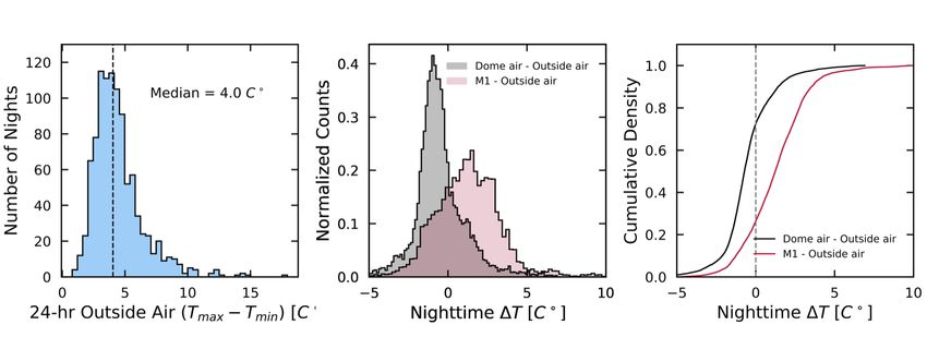
Turbulence can be parameterized in several ways. The amount of power in phase variations in each spatial
or temporal Fourier mode, called the power spectral density (PSD), is one metric. The PSD of atmospheric
turbulence is generally assumed to follow the Von Karman spectrum;18 for simplicity, we assume a scale-free
Kolmogorov spectrum:19–22
                                               P SD = 10α f β                                           (1)
where f are Fourier modes, 10α is the amplitude of the PSD, and β is the power-law index of the PSD. We use
the following convention to distinguish between spatial and temporal PSD parameters: spatial PSD parameters
are denoted with a subscript “s”, while temporal PSD parameters are denoted with a subscript “t”. The rate
at which energy is transferred from large scale eddies to smaller scale eddies is embodied in β. In frozen flow
turbulence,23 βs = −11/3 and βt = −8/3.24 This assumption implies that a single layer of turbulence can be
regarded as fixed phase screen propagating horizontally through the atmosphere. The strength and speed of the
turbulence is frequently distilled into two parameters: the coherence length and the coherence time, respectively
denoted as r0 and τ0 . The coherence length, also called the Fried parameter, describes the lateral distance across
the aperture in which the RMS phase aberration of the incoming wavefront is one radian. The full width at half
maximum (FWHM) of the PSF, also called the seeing disk, is 0 ∼ λ/r0 where λ is the observing wavelength. The
coherence time, τ0 ∝ r0 /v0 , where v0 is the characteristic velocity of the turbulence. AO systems are generally
designed using these turbulence models with assumptions about the local r0 and τ0 values of the observatory.15
If any of these assumptions are violated, there is a risk of under-designing the system in some aspect, whether
it is deformable mirror stroke budget or loop speed.
    Turbulence introduced in and around the telescope dome can lead to mediocre performance on nights with
otherwise exceptional observing conditions. We use the general term “dome seeing” to refer to any source
of additional turbulence in the dome and “mirror seeing” to refer to turbulence sourced specifically from the
telescope mirror(s). Studies done with seeing-limited instruments found that the PSF FWHM and Strehl Ratio
(the ratio of the peak PSF intensity to that of a perfect Airy pattern) are strongly correlated with temperature
differences throughout the dome.25, 26 Furthermore, laboratory studies observed that mirror seeing develops as
soon as the mirror’s temperature exceeds the ambient air temperature.27 Recent results from Robo-AO are also
suggestive of the effects of dome seeing on AO instrumentation.28 Anecdotally, some GPI data sets have shown
poorer performance on nights with otherwise exceptional seeing conditions, as measured by the observatory
seeing monitors. This motivates the need for a study of mirror seeing that pertains to high-contrast imaging.
Although, we limited our study to a single instrument, these results could also be generalized to other Gemini
instruments such as GEMS or ALTAIR and likely to other observatories as well.
    According to the above studies, the key to reducing dome seeing is to control the temperature inside the dome.
For the past few years, the temperature control strategy at GS has been to measure the outside air temperature
near the start of each night, then use that temperature as the set point for the dome air conditioning for the
following afternoon. This strategy performs well when the weather is stable, but it is not ideal when weather
fronts cause rapid changes in temperature from one day to the next. The primary mirror (M1) temperature is
not actively controlled, and is often considerably warmer than the outside air, as it is a large, heavy structure
with a much slower cool-down rate.
    In this work, we investigate the effects of mirror seeing on AO performance, using data from the The Gemini
Planet Imager Exoplanet Survey (GPIES).29 GPIES is a direct imaging campaign that began in 2014 to search
for exoplanets and circumstellar disks around ∼600 young, nearby stars. Each campaign observation is archived
together with observatory environmental metadata and AO telemetry. This large, uniform dataset enables
us to study the relationship between various environment and telescope parameters with GPI performance.
Additionally, we can do a more detailed analysis of mirror turbulence with the AO telemetry data. The datasets
used in this study are described in Section 2. The filtering and matching of datasets as well as the techniques
used to calculate turbulence parameters are described in Section 3. Our results are presented and discussed in
Section 4. We conclude in Section 5.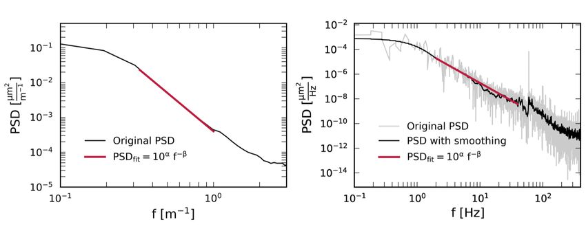
2. DATA
2.1 GPIES observations
A GPIES campaign observation is comprised of 20 – 40 sequential H-band (1.6 µm) integral field spectrograph
(IFS) images, each with a 60 second exposure. Each exposure is automatically reconstructed into a spectral cube
(x, y, λ), which we refer to as “raw images.” A record of the instrument, observatory, and ambient environment
states, along with a time stamp and target identification information are saved in the image header. At the end
of an observing sequence, individual raw IFS images automatically undergo calibration and PSF-subtraction and
are combined into a single “final” IFS image by the GPIES data pipeline.30–33
An important metric used for monitoring GPI’s performance is contrast, the minimum detectable planet-to-
star flux ratio at a given projected separation from the host star. The 5σ contrast at a given separation is defined
as five times the local standard deviation of the noise in an annulus centered at that separation. This calculation
first takes place for each wavelength slice in a cube, and then the values for the central 50% of the spectral band
are median-combined to produce a single contrast curve that is associated with the observation.31, 33 Typical
“raw contrast” values at 0.400 are . 10−4 . The “final contrast” is typically 10-50 times better than the raw
contrast.
The raw and final data products are logged in the GPIES database as they are produced.34 This includes
the raw and final 5-σ contrast measured at 0.200 , 0.400 , and 0.800 separations. For simplicity, we consider only the
raw and final contrast at 0.400 separation. At smaller separations performance can be affected by coronagraph
misalignment, and at larger separations images may be background limited.11 In total, we have access to 28,387
raw images and 719 final images, which were gathered between November 2014 and January 2019.
2.2 GPI AO telemetry
GPI’s AO system10 consists of a Shack-Hartmann wavefront sensor (WFS) and two deformable mirrors (DMs).
The WFS uses 2 x 2 pixel quad-cell centroiding to measure the slope of the wavefront across each subaperture
in the full telescope aperture, which is 43 subapertures wide. Each subaperture samples 18 cm of the wavefront
and these measurements are performed at a rate of 1 kHz on stars brighter than 8th magnitude in I-band, and
500 Hz on fainter stars. The phase of the wavefront is reconstructed in Fourier modes.35 Low-order modes are
sent to the woofer DM and the tip/tilt stage, high-order modes are sent to the tweeter DM. The realtime control
computer estimates the modal coefficients for tip, tilt, and focus and removes them from the signal that drives
the control loop.
Several types of AO data are periodically recorded for analysis purposes, 2–5 times per target, at the discretion
of the observer. A full telemetry set contains a record of the WFS measurements, DM and tip/tilt commands,
along with any other offsets applied. The datasets used here are 10–22 sec long, and a total number of 2009 AO
telemetry sets were recorded between September 2014 and January 2019.
A direct measurement of the AO system’s performance is the residual wavefront error (σWFE ), defined as the
error measured by the WFS after applying a correction with the DM. An instantaneous approximation of σWFE ,
based on the RMS subaperture slopes, is saved to the header of each raw IFS frame (See Section 3.1). We also
estimated the σWFE from reconstructed wavefront telemetry as discussed in Section 3.2.
2.3 Gemini observatory data
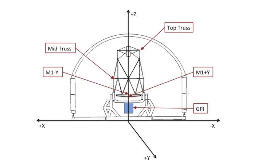
There are multiple temperature sensors placed in and around the telescope dome at GS. Each sensor records
the temperature every five minutes. The approximate location of the interior sensors relevant to this study
are displayed in Figure 1. At each location there is one sensor directly attached to the metal truss surface
(Minco S651PDX24B36 ) and another that is suspended freely in the air next to it (Omega RDT-80537 ). On
M1, there are two individual sensors mounted directly on the outer rim. The “M1-Y” sensor is attached to the
side that tips downwards when the telescope slews to lower elevation, while the “M1+Y” sensor is attached to
the side that tips upwards. The precision of the temperature data is ∼ 1% at 25 ◦ C, according to the sensor
specifications. Although precise, the sensors may be subject to constant bias offsets, as will be discussed in
Section 3.1. Additionally, the outside air temperature is recorded by a weather tower adjacent to GS.Figure 1. Schematic of Gemini South telescope and observatory dome. Arrows mark the location of temperature sensors.
The 0 and τ0 values at the time of observation were provided by the observatory’s Differential Image Motion
Monitor (DIMM) and Multi-Aperture Scintillation Sensor (MASS), respectively.38 These instruments are not
located in the dome, but rather in a separate tower ∼80 m away. Consequently, they are insensitive to mirror
or dome seeing, a crucial point for our study.
3. METHODS
3.1 Filtering, matching, and calibrating GPI science data and temperature readings
IFS raw and final datasets were filtered as follows. To ensure high signal-to-noise images and telemetry, we
included in our sample only bright stars (I-band magnitude < 7). This also guaranteed that the AO system
was operating at 1 kHz for all images in the sample. We also excluded images that were taken in the worst
seeing conditions or when there was no recent measurement (. 40 min) from the MASS/DIMM. According to
the MASS/DIMM, the median seeing recorded at Cerro Pachon from the years 2014 to 2019 was 0 = 0.900 and
τ0 = 1.5 ms. We only kept the images corresponding to the best 85% seeing conditions:0 < 1.200 and τ0 > 0.8 ms.
These seeing cuts combined culled almost 80% of the remaining dataset, in large part because no MASS/DIMM
values were available after early 2017. Next, we rejected final images where the field of view (FOV) rotated by
less than twice the FWHM of the PSF for a planet orbiting its star at 0.400 (θFOV > 12.2◦ )∗ . The final contrast
depends the FOV rotation because the GPI data pipeline relies in part on the angular differential imaging
observing technique. Sequences with a lower FOV rotation suffer loss of sensitivity due to self-subtraction during
the PSF subtraction process. After all of these cuts, 2,977 raw frames and 120 final images remained. The
remaining data represent 57 different observing nights between September 2014 and February 2017.
Lastly, not all sequences attained the same total integration
p time. To normalize all values to an equivalent
of a full sequence (38 min), we scaled final contrast by ti /38 min, where ti is the total integration time. This
scaling was verified to hold after the minimum θFOV was achieved, based on a multi-hour c Eri dataset.
The approximate σWFE that is stored in the IFS headers is overestimated because the calibration between
the RMS displacement of the WFS centroids and the actual wavefront error was never measured. We obtained
the linear relationship:
σAO telemetry = (81.01 ± 0.02)10−2 σIFS header − (20 ± 4) [nm RMS] (2)
∗
θFOV > 2λ
Dρ
, where λ = 1.65 µm, D = 8 m, and ρ = 0.400 .Figure 2. Comparison of residual wavefront error derived from AO telemetry, σAO telemetry , to the instantaneous approx-
imation saved to the IFS image headers, σIFS header (black points). The linear fit is overlaid (red line), and was used to
correct σIFS header in subsequent analysis.
using a subset of images that had contemporaneous residual phase maps reconstructed from full AO telemetry
(as described in Section 3.2). The data and fit are displayed in Figure 2. We corrected all IFS header values
using this fit.
We also filtered and calibrated the GS temperature data. Bad or missing data in the GS temperature logs
are recorded with a null value; these entries were removed. We cross-checked the M1 temperatures against
simultaneous readings from the GPI AO bench temperature sensor and the dome air and truss sensors. Both
M1 sensors revealed significant offsets. The observatory staff calibrated these two sensors on August 3, 2017.
Unfortunately, the offsets were not recorded during the calibration process. To correct the historical data, we
determined the zero-point offset for each sensor in the following way: first, we split the data into before and after
calibration sets; from January 1, 2014 to August 2, 2017 and from August 4, 2017 to December 31, 2018, and
then folded them by year. Next, we fit a line to the before calibration data from August 4, to December 31 and
subtracted the fit from the after calibration data. In the final step, we calculated the DC offset that made the
mean of the difference equal to zero. The average offset value for each sensor is displayed in Table 1. The dome
air temperature reported by the various truss air temperature sensors also showed moderate systematic offsets.
The lower-truss sensor reading most closely matched the temperature reported by the weather tower, while the
upper- and mid-truss sensors reported temperatures 1 − 2 ◦ C cooler. Because the calibration of these sensors
were not independently checked, as M1 sensors were, we chose to use only the readings from the lower-truss
sensor. We stress, however, that absolute temperatures were not essential in this study, as we investigated only
the relationship between GPI performance and relative temperature changes.
Table 1. Calculated temperature offsets for GS temperature sensors (Tcorrected = T0 + offset).
Sensor Offset [◦ C]
M1+Y 3.5
M1-Y 2.1
Ultimately, a single value of each environment parameter (M1 temperature, dome temperature, τ0 , and 0was associated with each raw and final image for all subsequent analysis. We averaged the two corrected M1
sensors to produce an instantaneous M1 temperature. We matched each raw science frame with its closest-in-time
temperature readings. If no temperature was recorded within thirty minutes of the observation, we excluded the
image from our sample; this removed ∼ 25 of the raw images. Finally, we matched final science frames with the
average M1 and dome temperatures and the average seeing recorded during the entire observation sequence.
3.2 Characterizing turbulence with AO telemetry
We quantified the characteristics of mirror turbulence by examining the spatial and temporal PSDs of the
wavefronts at the entrance pupil (ie: before AO correction). In theory it is possible to directly measure mirror
seeing with open-loop measurements from the WFS. But in practice, open-loop wavefront errors are too large
to be measured by GPI’s WFS. Thus, rather than directly measuring the open-loop phase, we reconstructed the
“pseudo open-loop” phase from closed-loop AO telemetry. A detailed description of this process can be found
in Reference 39 and in Reference 40. The closed-loop residual phase measured by the WFS, ΦWFS , is given by:
ΦWFS = ΦA − ΦDM , (3)
where ΦA is the pseudo open-loop phase and ΦDM is the DM commanded phase. Each pseudo open-loop time
series was mapped onto a slightly oversized cube containing (48 x 48) subapertures x 22,000 ms, with a pixel
scale of 0.18 m at M1. Any uncontrolled data points, such as those located outside the aperture area, on the
aperture edge, or behind the secondary mirror were set to zero.
Tip and tilt were already removed from the signal by the realtime control computer; however some static
aberrations remained. To estimate the low-order static aberrations, we calculated the time-average phase map
and fit it with the first six Zernike polynomials, under the assumption that any low-order turbulence-induced
wavefront error would average to zero over the 10-22 second time series. We used the python optical simulation
package Poppy41 to calculate normalized Zernike coefficients.
We then used the 2D Discrete Fourier Transform (DFT) to decompose the phase signal at each timestep into
its Fourier modes. Given the open loop phase φ(x, y, ti ) and the aperture a(x, y), the modal coefficients at each
time step ti are
N −1 N −1
1 X X
Fxy (kx , ky , ti ) = PN −1 PN −1 φ(x, y, ti )a(x, y)e−2πj(kx x+ky y) (4)
x=0 y=0 a(x, y) x=0 y=0
Computing the square of the spatial modes, yields the spatial PSD, which is the following:
Pxy (kx , ky ) = h|Fxy (kx , ky , t)|2 it (5)
where hit is the time-average of the individual PSDs. An example of the spatial PSD (left) and the temporal
PSD (right) of the turbulence recorded while observing c Eri on 12/19/2015 is shown in Figure 3.
The length scales captured by GPI range from 0.36 m to 8 m, where 0.36 m is twice one subaperture diameter
and 8 m is the full aperture diameter. We fit a power law of the form PSD = 10αs f βs from the middle region of
the spectrum (0.3 m−1 , 1.0 m−1 ), which is highlighted in Figure 3. This selection ensures that our parameters
are free from tilt and outer scale effects at lower spatial frequencies and WFS aliasing effects at higher spatial
frequencies.
This process was repeated to estimate the average temporal PSD of the DM actuators:
Pt (ω) = h|Ft (x, y, t)|2 ixy , (6)
where hixy is the average of all the DM actuators in the aperture and the DFT of each time series is equal to:
N −1
1 X
Ft (ω) = φ(x, y, t)a(x, y)e−2πj(ωt) . (7)
N t=0(a) (b)
Figure 3. Spatial (left) and temporal (right) PSDs of pseudo open-loop wavefront errors derived from AO telemetry
recorded while observing c Eri on 12/19/2015. We superimposed the temporal PSD obtained after applying the Savitzky-
Golay filter (black) with the original temporal PSD (grey).
Power law fits (red line) were performed in the inertial range of the PSDs.
The resulting temporal PSD, which is displayed in Figure 3 on the right, appears noisier than the spatial PSD
because the position of each DM actuator is more finely sampled than the spatial modes. Thus, we used a
Savitzky-Golay42 filter with a window length of 101 ms and polynomial order of 5 to reduce the noise in the
temporal PSD. The Savitzky-Golay filter splits the data into discrete segments and approximates the data inside
each interval with a polynomial fit. After we smoothed the PSD, we fit a power law of the form PSD = 10αt f βt
from (2 Hz, 40 Hz)to avoid potential biases associated with aliasing and/or vibrations that may be introduced
by the telescope.
(a) (b) (c)
Figure 4. Temperatures at the Gemini South observatory. (a) Histogram of the daily min-max range of outside air
temperatures. (b) Histogram of instantaneous temperature differences between dome air or M1 and outside air at night,
for those nights when GPI was observing, with DC offset corrections as described in Section 3.1. (c) Cumulative density
plot of the data in (b)4. RESULTS
4.1 Temperature conditions at Gemini South
We first investigated the typical temperature conditions at GS using temperature records from the years 2015–
2019, which include all nights, not only those with GPI data. We excluded nights with only partial records. We
required at least 10 measurements recorded in a 24 hr period, and at least four hours between Tmax and Tmin .
A total of 1001 nights, out of an original 1221, remained. Figure 4(a) shows a histogram of (Tmax − Tmin ) of the
outside air for each calendar day, split at sunset. The distribution peaks at 4 ◦ C, but occasionally reaches 15 ◦ C,
illustrating the wide range of day-night temperature swings that the observatory must cope with. We measured
the nighttime instantaneous temperature differences between M1, dome air, and ambient air, in order to identify
potential sources of dome seeing. We only considered nights in which GPI took on-sky data. We plot their density
histograms in figure 4 (b), and their cumulative densities in figure 4 (c). The reported median temperature of
the dome is 0.7 ◦ C cooler than ambient while the reported median temperature of M1 is 1.2 ◦ C warmer than
ambient. However, as discussed previously, while the calibration of the M1 sensors has been validated, those
of the outside air sensor and the dome air sensor have not. Thus, while the distributions of dome-ambient
and M1-ambient difference are correct, the medians could be biased. From the standard deviations of the two
distributions (1.6 ◦ C and 2.0 ◦ C respectively), we can conclude that the dome more quickly tracks ambient
temperature than M1.
Figure 5 shows the median 24-hour temperature profile of M1, dome air, and outside air for nights in which
GPI took on-sky data. It shows that the min–to–max range of M1 is small compared to the min–to–max range
of the ambient air. We postulate that M1 typically remains warmer than ambient air during the night, resulting
in additional “mirror seeing” and in GPI AO performance degradation. The exact thermal balance of any
observatory is complex. M1 may never be in good equilibrium after sudden jumps in the ambient temperature,
which on Cerro Pachon are frequently > 4 ◦ C in a day. There could also be potential sources of heat such as
electronics in or near the mirror cell. This is an ongoing area of study at the Gemini Observatory.
Figure 5. Median 24-hour temperature profile at GS for nights on which GPI took on-sky data. The black, red, and blue
lines represent the median temperature of M1, dome air, and the outside air. Vertical dashed lines mark the approximate
length of the shortest and longest nights of the year.4.2 Effect of temperature differentials on residual wavefront error and contrast
Next we explored the correlation between the instantaneous σWFE recorded in the GPI image headers and the
temperature differences between M1 and the outside air. The result, which is displayed in Figure 6, shows
that σW F E becomes larger as the temperature difference between M1 and the outside air increases. Some
vertical scatter is present due to additional contributions from other sources affecting performance, such as stellar
magnitude or atmospheric seeing conditions. With appropriate calibration, measurements from the observatory
seeing monitors could potentially be used to correct for some of the atmospheric seeing contribution; this analysis
is left to future work. Nonetheless, the performance limit imposed by mirror seeing is clearly captured by the
lower envelope of the data, which corresponds to the best seeing conditions. The model43 we used to capture
the relationship between σW F E and ∆TM is:
σW F E = a|∆TM | + b (8)
where a and b are free parameters. To isolate the impact of ∆TM , we only fit the bottom 25th percentile of each
0.5 ◦ C temperature difference bin. The resulting fit is:
σW F E = (13.9 ± 0.4) |∆TM | + (47.5 ± 0.7) [nm RMS] (9)
Our fit predicts that we obtain an additional 41.6 ± 1.2 nm of wavefront error when M1 is 3◦ C warmer than the
outside air. This behavior is consistent with results from previous studies of mirror seeing25–27 when ∆TM > 0◦ C.
Past studies observed a weaker effect at ∆TM < 0◦ C. Our data are consistent with an equal slope at both warmer
and cooler temperatures, although hints of a weaker effect at cooler temperatures are present. We note that our
data span a larger range of negative temperatures than most previous studies.
Figure 6. σWFE vs. ∆TM . The temperature difference between M1 and ambient sets the lower limit on σWFE . The red
line indicates a fit of the bottom 25th percentile of the data, which are the points shaded in black.
We also quantified the effects of mirror seeing on contrast performance, which is the quantity of interest when
imaging planets. Previous correlation studies of GPI performance showed that raw contrast and final contrast
2
both scaled with σWFE at close-to-intermediate separations.10, 11 Therefore, we expected that raw contrast and
final contrast to have the following relationship:
Contrast at 0.400 = c ∆TM
2
+d (10)where c and d are free parameters. Figure 7 displays raw contrast (left) and final contrast (right) plotted as a
function of ∆TM . Once again we see that the temperature difference sets a floor to the achievable contrast. For
both raw and final contrast, we again fit only the bottom 25th percentile of each 0.5 ◦ C temperature difference
bin. The fit for raw contrast is:
Contrast at 0.400 = (7.3 ± 0.1)10−6 ∆T2M + (3.6 ± 0.1)10−5 , (11)
and the fit for final contrast is:
Contrast at 0.400 = (3.4 ± 0.6)10−7 ∆T2M + (1.4 ± 0.3)10−6 . (12)
Our fits show that when M1 is 3 ◦ C warmer than the outside air, both raw and contrast degrade by a factor of 3±1.
This is an apparent discrepancy with Reference 44 results for the Keck/NIRC2 Vortex Coronagraph instrument
performance, which did not find a relationship between achievable contrast and temperature differences. However,
an overwhelming majority of their data had ∆TM < 0.5 ◦ C, where we see only a very weak effect. Furthermore,
Reference 44 fit all of their data, not only the best 25th percentile. We believe these two factors account for the
apparent discrepancy.
(a) (b)
Figure 7. Image contrast vs. ∆TM . (a) is raw contrast while (b) is final contrast. Blue line is the fit of the best 25th
percentile of the data (black points). On nights when the temperature of the mirror diverged by more than 3 ◦ C from
the outside air temperature, both raw and final contrast degraded by ∼ 3 ×.
4.3 Effect of temperature differentials on turbulence power spectra
Evidently high-contrast imaging performance is reduced significantly when M1 is not in thermal equilibrium;
however this relationship alone cannot identify the underlying cause. As discussed in Section 1, GPI’s AO
system was designed assuming Kolmogorov turbulence models of the local atmosphere. Perhaps M1 is an extra
source of turbulence, resulting in turbulence conditions for which the AO system is no longer optimized. The
GS seeing monitors, located outside the dome, cannot directly measure mirror turbulence. However, GPI’s
well-characterized AO system may be able to. In this section, we check for relationships between the structure
of the spatial and temporal PSDs and ∆TM measured during the entire GPIES campaign. The spatial PSD
is calculated with all temporal frequencies, and we fit only spatial frequencies between 0.3 m−1 and 1.0 m−1 .The temporal PSD is calculated using all spatial frequencies, and we fit only temporal frequencies between 2 hz
and 40 hz. Therefore, keep in mind that we cannot rule out effects at other length scales or frequencies. After
the data selection outlined in Section 3.1, a total of 582 AO telemetry sets remained. We then averaged the
parameters that were extracted from the fits for all telemetry sets taken while integrating on the same star,
leaving 122 measurements.
The parameters extracted from our fits, log(α) and (β), are plotted as a function of ∆TM in Figure 8. We
find that there is no clear dependence between β and ∆TM . The βs data are uniformly scattered on the expected
power-law for spatial Kolmogorov turbulence (−11/3), indicating that mirror seeing does not exhibit significant
deviations from Kolmogorov behavior at these length scales. The βt data also exhibits uniform behavior, but at
a slightly higher value than the expected power-law for temporal Kolmogorov turbulence (−8/3). This shows
that the temporal power spectrum is flatter than what is expected from Kolmogorov, implying an excess of high
temporal frequencies with respect to simply translating a Kolmogorov phase screen. Disentangling the relative
contributions of noise vs. small-spatial-scale boiling is left to future work.
Now we focus on α, which is directly related to the total seeing.45 We expect the total seeing to increase as
the mirror temperature difference increases, and indeed we find a positive trend between αs and ∆TM , albeit at
low signal to noise. This, combined with the flat dependence of βs on ∆TM tells us that the power spectrum is
shifted vertically upwards when ∆TM increases, implying that the intensity of turbulence gets increased at all
length scales in the inertial range. Surprisingly, this behavior is less obvious with αt , but we hypothesize that
our inability to probe smaller length scales and/or other noise sources could be obscuring the trend.
5. CONCLUSION
In this analysis we studied the effect of the temperature difference (∆TM ) between the primary mirror (M1) and
the outside air, a proxy for “mirror seeing,” on the performance of the Gemini Planet Imager at the Gemini
South Observatory. Our analysis included 2,977 60 sec single exposures, 120 fully reduced observing sequences,
and 582 AO telemetry sets recorded between September 2014 and February 2017 during the GPIES campaign,
as well contemporaneous temperature and atmospheric seeing measurements. We found that M1 is often warmer
than ambient temperature.
We demonstrated that GPI’s sensitivity to planets is directly impacted by these temperature differences.
Indeed, the best single image (“raw”) contrast and full sequence (“final”) contrast performance occurred when
∆TM was closest to 0 ◦ C. The raw and final image contrasts degrade by a factor 3 ± 1 when ∆TM = 3 ◦ C. We
also analyzed the spatial and temporal PSDs derived from AO system telemetry by fitting a power-law to the
inertial region of the spectrum (0.3 m−1 and 1.0 m−1 ) and (2 Hz and 40 Hz). We found that “mirror seeing”
increased the intensity of turbulence at all length scales in the inertial range, as evidenced by the increase in the
spatial PSD amplitude (αs ) with ∆TM . We also found that in these frequencies ”mirror seeing” was neither more
nor less Kolmogorov than turbulence measured when M1 was in equilibrium with the ambient air. Lastly, all
datasets showed some deviations from 1-layer frozen-flow expectations; the root cause of which is left to future
work.
We argue that improvements to the GS dome air and mirror temperature control strategies could improve
performance of GPI and other adaptive optics instruments. A possible remediation could involve actively cooling
M1 during the day with cooling plates behind the glass, which are capable of lowering M1’s temperature by
1◦ C/hr.46 Alternatively, some studies have shown that slowly blowing a stream of cold air above the mirror
surface may reduce mirror seeing effects,26 although this technique has not been tested in high-contrast imaging
applications. The observatory staff at GS are continuing to investigate the issue and are in the process of
installing a cross-primary laser system that will measure M1 seeing directly.
Our results are generalizable to general-purpose AO systems.
√ The factor of 3 contrast degradation that GPI
sees when ∆TM = 3 ◦ C roughly corresponds to a factor of 3 increase in wavefront error. Telescope temperature
control is critical for maximizing the performance of any AO instrument.Figure 8. Power law index (β) and log(amplitude (α)) derived from fits of spatial and temporal PSDs are plotted as a
function of ∆TM . The points are the mean of each campaign sequence. The black points highlight those datasets with the
best 25th percentile contrast, as defined in Figure 7. The power law expected for spatial Kolmogorov turbulence (-3.67)
and for temporal Kolmogorov turbulence (-2.67) is marked with a line. Only the strength of the turbulence as measured
by the spatial PSD shows clear dependence on ∆TM .
6. ACKNOWLEDGEMENTS
The GPI project has been supported by Gemini Observatory, which is operated by AURA, Inc., under a coop-
erative agreement with the NSF on behalf of the Gemini partnership: the NSF (USA), the National Research
Council (Canada), CONICYT (Chile), the Australian Research Council (Australia), MCTI (Brazil) and MIN-
CYT (Argentina). Additionally, portions of this work were performed under the auspices of the U.S. Department
of Energy by Lawrence Livermore National Laboratory under Contract DE-AC52-07NA27344. Vanessa P. Bailey
acknowledges government sponsorship; this research was carried out in part at the Jet Propulsion Laboratory,
California Institute of Technology, under a contract with the National Aeronautics and Space Administration.
We thank the referees for their helpful comments and we thank the following people for their contributions
to this project; Alex Madurowicz, Varun Harbola, Claire Hebert, Adam Snyder, Eric Nielsen, Jerome Maire, LeaA. Hirsch, and Robert De Rosa.
REFERENCES
[1] Marois, C., Macintosh, B., Barman, T., Zuckerman, B., Song, I., Patience, J., Lafrenière, D., and Doyon,
R., “Direct Imaging of Multiple Planets Orbiting the Star HR 8799,” Science 322, 1348 (Nov 2008).
[2] Nielsen, E. L., Liu, M. C., Wahhaj, Z., Biller, B. A., Hayward, T. L., Males, J. R., Close, L. M., Morzinski,
K. M., Skemer, A. J., and Kuchner, M. J., “The Gemini NICI Planet-Finding Campaign: The Orbit of the
Young Exoplanet β Pictoris b,” Astrophysical Journal 794, 158 (Oct 2014).
[3] Macintosh, B., Graham, J. R., Barman, T., De Rosa, R. J., Konopacky, Q., Marley, M. S., Marois, C.,
Nielsen, E. L., Pueyo, L., and Rajan, A., “Discovery and spectroscopy of the young jovian planet 51 Eri b
with the Gemini Planet Imager,” Science 350, 64–67 (Oct 2015).
[4] Bowler, B. P., “Imaging Extrasolar Giant Planets,” Proceedings of the Astronomical Society of the Pa-
cific 128, 102001 (Oct 2016).
[5] Rajan, A., Rameau, J., De Rosa, R. J., Marley, M. S., Graham, J. R., Macintosh, B., Marois, C., Morley,
C., Patience, J., and Pueyo, L., “Characterizing 51 Eri b from 1 to 5 µm: A Partly Cloudy Exoplanet,”
Astronomical Journal 154, 10 (Jul 2017).
[6] Keppler, M., Benisty, M., Müller, A., Henning, T., van Boekel, R., Cantalloube, F., Ginski, C., van Holstein,
R. G., Maire, A. L., and Pohl, A., “Discovery of a planetary-mass companion within the gap of the transition
disk around PDS 70,” Astronomy and Astrophysics 617, A44 (Sep 2018).
[7] Stone, J. M., Skemer, A. J., Hinz, P. M., Bonavita, M., Kratter, K. M., Maire, A.-L., Defrere, D., Bailey,
V. P., Spalding, E., and Leisenring, J. M., “The LEECH Exoplanet Imaging Survey: Limits on Planet
Occurrence Rates under Conservative Assumptions,” Astronomical Journal 156, 286 (Dec 2018).
[8] Soummer, R., Sivaramakrishnan, A., Oppenheimer, B. R., Roberts, R., Brenner, D., Carlotti, A., Pueyo,
L., Macintosh, B., Bauman, B., and Saddlemyer, L., “The Gemini Planet Imager coronagraph testbed,” in
[Techniques and Instrumentation for Detection of Exoplanets IV ], Society of Photo-Optical Instrumentation
Engineers (SPIE) Conference Series 7440, 74400R (Aug 2009).
[9] Macintosh, B., Graham, J. R., Ingraham, P., Konopacky, Q., Marois, C., Perrin, M., Poyneer, L., Bauman,
B., Barman, T., and Burrows, A. S., “First light of the Gemini Planet Imager,” Proceedings of the National
Academy of Science 111, 12661–12666 (Sep 2014).
[10] Poyneer, L. A., Palmer, D. W., Macintosh, B., Savransky, D., Sadakuni, N., Thomas, S., Véran, J.-P.,
Follette, K. B., Greenbaum, A. Z., and Mark Ammons, S., “Performance of the Gemini Planet Imager’s
adaptive optics system,” Applied Optics 55, 323 (Jan 2016).
[11] Bailey, V. P., Poyneer, L. A., Macintosh, B. A., Savransky, D., Wang, J. J., De Rosa, R. J., Follette,
K. B., Ammons, S. M., Hayward, T., and Ingraham, P., “Status and performance of the Gemini Planet
Imager adaptive optics system,” in [Adaptive Optics Systems V], Society of Photo-Optical Instrumentation
Engineers (SPIE) Conference Series 9909, 99090V (Jul 2016).
[12] Milli, J., Mouillet, D., Fusco, T., Girard, J., Masciadri, E., Pena, E., Sauvage, J.-F., Reyes, C., Dohlen, K.,
Beuzit, J.-L., Kasper, M., Sarazin, M., and Cantalloube, F., “Performance of the extreme-ao instrument
vlt/sphere and dependence on the atmospheric conditions,” AO4ELT5 Conference Series 10.26698, 34
(2017).
[13] Racine, R., Walker, G. A. H., Nadeau, D., Doyon, R., and Marois, C., “Speckle Noise and the Detection of
Faint Companions,” Proceedings of the Astronomical Society of the Pacific 111, 587–594 (May 1999).
[14] Perrin, M. D., Sivaramakrishnan, A., Makidon, R. B., Oppenheimer, B. R., and Graham, J. R., “The
Structure of High Strehl Ratio Point-Spread Functions,” Astrophysical Journal 596, 702–712 (Oct 2003).
[15] Madurowicz, A., Macintosh, B. A., Ruffio, J.-B., Chilcote, J., Bailey, V. P., Poyneer, L., Nielsen, E., and
Norton, A. P., “Characterization of lemniscate atmospheric aberrations in Gemini Planet Imager data,”
in [Adaptive Optics Systems VI], Society of Photo-Optical Instrumentation Engineers (SPIE) Conference
Series 10703, 107036E (Jul 2018).
[16] Cantalloube, F., Por, E. H., Dohlen, K., Sauvage, J. F., Vigan, A., Kasper, M., Bharmal, N., Henning,
T., Brandner, W., Milli, J., Correia, C., and Fusco, T., “Origin of the asymmetry of the wind driven halo
observed in high-contrast images,” Astronomy and Astrophysics 620, L10 (Dec 2018).[17] Milli, J., Kasper, M., Bourget, P., Pannetier, C., Mouillet, D., Sauvage, J. F., Reyes, C., Fusco, T., Can-
talloube, F., and Tristam, K., “Low wind effect on VLT/SPHERE: impact, mitigation strategy, and results,”
in [Adaptive Optics Systems VI], Society of Photo-Optical Instrumentation Engineers (SPIE) Conference
Series 10703, 107032A (Jul 2018).
[18] de Karman, T. and Howarth, L., “On the Statistical Theory of Isotropic Turbulence,” Proceedings of the
Royal Society of London Series A 164, 192–215 (Jan 1938).
[19] Fried, D. L., “Limiting Resolution Looking Down Through the Atmosphere,” Journal of the Optical Society
of America (1917-1983) 56, 1380 (Oct 1966).
[20] Hardy, J. W., [Adaptive Optics for Astronomical Telescopes], Oxford University Press (1998).
[21] Tatarskii, V. I., [Wave Propagation in Turbulent Medium], Dover books on physics and mathematical
physics, Dover (1961).
[22] Roddier, F., “The effects of atmospheric turbulence in optical astronomy,” Progess in Optics 19, 281–376
(Jan 1981).
[23] Taylor, G. I., “The Spectrum of Turbulence,” Proceedings of the Royal Society of London Series A 164,
476–490 (Feb 1938).
[24] Conan, J. M., Rousset, G., and Madec, P. Y., “Wave-front temporal spectra in high-resolution imaging
through turbulence.,” Journal of the Optical Society of America A 12, 1559–1570 (Jul 1995).
[25] Racine, R., Salmon, D., Cowley, D., and Sovka, J., “Mirror, Dome, and Natural Seeing at CFHT,” Proceed-
ings of the Astronomical Society of the Pacific 103, 1020 (Sep 1991).
[26] Lowne, C. M., “An investigation of the effects of mirror temperature upon telescope seeing.,” Monthly
Notices of the Royal Astronomical Society 188, 249–259 (Jul 1979).
[27] Iye, M., Noguchi, T., Torii, Y., Mikami, Y., and Ando, H., “Evaluation of Seeing on a 62-cm Mirror,”
Proceedings of the Astronomical Society of the Pacific 103, 712 (Jul 1991).
[28] Jensen-Clem, R., Duev, D. A., Riddle, R., Salama, M., Baranec, C., Law, N. M., Kulkarni, S. R., and
Ramprakash, A. N., “The Performance of the Robo-AO Laser Guide Star Adaptive Optics System at the
Kitt Peak 2.1 m Telescope,” Astronomical Journal 155, 32 (Jan 2018).
[29] Nielsen, E., De Rosa, R., Macintosh, B., Wang, J., Ruffio, J.-B., Chiang, E., Marley, M., Saumon, D.,
Savransky, D., Fabrycky, D., Konopacky, Q., Patience, J., and Bailey, V., “The Gemini Planet Imager
Exoplanet Survey: Giant Planet and Brown Dwarf Demographics from 10-100 AU,” in [AAS/Division for
Extreme Solar Systems Abstracts], AAS/Division for Extreme Solar Systems Abstracts 51, 100.02 (Aug
2019).
[30] Perrin, M. D., Maire, J., Ingraham, P., Savransky, D., Millar-Blanchaer, M., Wolff, S. G., Ruffio, J.-B.,
Wang, J. J., Draper, Z. H., and Sadakuni, N., “Gemini Planet Imager observational calibrations I: Overview
of the GPI data reduction pipeline,” in [Ground-based and Airborne Instrumentation for Astronomy V],
Society of Photo-Optical Instrumentation Engineers (SPIE) Conference Series 9147, 91473J (Jul 2014).
[31] Wang, J. J., Ruffio, J.-B., De Rosa, R. J., Aguilar, J., Wolff, S. G., and Pueyo, L., “pyKLIP: PSF Subtraction
for Exoplanets and Disks,” (Jun 2015).
[32] Perrin, M. D., Ingraham, P., Follette, K. B., Maire, J., Wang, J. J., Savransky, D., Arriaga, P., Bailey, V. P.,
Bruzzone, S., and Chilcote, J. K., “Gemini Planet Imager observational calibrations XI: pipeline improve-
ments and enhanced calibrations after two years on sky,” in [Ground-based and Airborne Instrumentation
for Astronomy VI ], Society of Photo-Optical Instrumentation Engineers (SPIE) Conference Series 9908,
990837 (Aug 2016).
[33] Ruffio, J.-B., Macintosh, B., Wang, J. J., Pueyo, L., Nielsen, E. L., De Rosa, R. J., Czekala, I., Marley,
M. S., Arriaga, P., and Bailey, V. P., “Improving and Assessing Planet Sensitivity of the GPI Exoplanet
Survey with a Forward Model Matched Filter,” Astrophysical Journal 842, 14 (Jun 2017).
[34] Wang, J. J., Perrin, M. D., Savransky, D., Arriaga, P., Chilcote, J. K., De Rosa, R. J., Millar-Blanchaer,
M. A., Marois, C., Rameau, J., and Wolff, S. G., “The automated data processing architecture for the GPI
Exoplanet Survey,” in [Society of Photo-Optical Instrumentation Engineers (SPIE) Conference Series ],
Society of Photo-Optical Instrumentation Engineers (SPIE) Conference Series 10400, 1040026 (Sep 2017).[35] Poyneer, L. A., Gavel, D. T., and Brase, J. M., “Fast wave-front reconstruction in large adaptive optics
systems with use of the Fourier transform,” Journal of the Optical Society of America A 19, 2100–2111 (Oct
2002).
[36] Minco, “Resistance thermometer, S651PDX24B.” https://www.minco.com/products/sense/
temperature/surfacesensor. (accessed: 06.10.2019).
[37] Omega, “Air temperature rtd sensors, RTD-805.” https://www.omega.com/en-us/
sensors-and-sensing-equipment/temperature/sensors/rtd-sensors/p/RTD-805-RTD-806. (ac-
cessed: 06.10.2019).
[38] Tokovinin, A. and Kornilov, V., “Accurate seeing measurements with MASS and DIMM,” Monthly Notices
of the Royal Astronomical Society 381, 1179–1189 (Nov 2007).
[39] Poyneer, L., van Dam, M., and Véran, J.-P., “Experimental verification of the frozen flow atmospheric
turbulence assumption with use of astronomical adaptive optics telemetry,” Journal of the Optical Society
of America A 26, 833 (Mar 2009).
[40] Srinath, S., Poyneer, L. A., Rudy, A. R., and Ammons, S. M., “Computationally efficient autoregressive
method for generating phase screens with frozen flow and turbulence in optical simulations,” Optics Ex-
press 23, 33335 (Dec 2015).
[41] Perrin, M., Long, J., Douglas, E., Sivaramakrishnan, A., and Slocum, C., “POPPY: Physical Optics Prop-
agation in PYthon.” Astrophysics Source Code Library (Feb. 2016).
[42] Savitzky, A. and Golay, M. J. E., “Smoothing and differentiation of data by simplified least squares proce-
dures,” Analytical Chemistry 36, 1627–1639 (Jan 1964).
[43] Tallis, M., Bailey, V. P., Macintosh, B., Chilcote, J. K., Poyneer, L. A., Ruffio, J.-B., Hayward, T. L.,
and Savransky, D., “Air, telescope, and instrument temperature effects on the Gemini Planet Imager’s
image quality,” in [Adaptive Optics Systems VI ], Society of Photo-Optical Instrumentation Engineers (SPIE)
Conference Series 10703, 1070356 (Jul 2018).
[44] Xuan, W. J., Mawet, D., Ngo, H., Ruane, G., Bailey, V. P., Choquet, É., Absil, O., Alvarez, C., Bryan,
M., and Cook, T., “Characterizing the Performance of the NIRC2 Vortex Coronagraph at W. M. Keck
Observatory,” Astronomical Journal 156, 156 (Oct 2018).
[45] Fétick, R. J. L., Fusco, T., Neichel, B., Mugnier, L. M., Beltramo-Martin, O., Bonnefois, A., Petit, C.,
Milli, J., Vernet, J., Oberti, S., and Bacon, R., “Physics-based model of the adaptive-optics-corrected point
spread function - applications to the sphere/zimpol and muse instruments,” A&A 628, A99 (2019).
[46] Greenhalgh, R. J. S., Stepp, L. M., and Hansen, E. R., “Gemini primary mirror thermal management
system,” in [Advanced Technology Optical Telescopes V], Stepp, L. M., ed., Society of Photo-Optical Instru-
mentation Engineers (SPIE) Conference Series 2199, 911–921 (Jun 1994).You can also read