Electron localisation descriptors in ONETEP: a tool for interpreting localisation and bonding in large-scale DFT calculations - IOPscience
←
→
Page content transcription
If your browser does not render page correctly, please read the page content below

Electronic Structure

TECHNICAL NOTE • OPEN ACCESS

Electron localisation descriptors in ONETEP: a tool for interpreting
localisation and bonding in large-scale DFT calculations
To cite this article: R J Clements et al 2020 Electron. Struct. 2 027001

View the article online for updates and enhancements.

                                This content was downloaded from IP address 46.4.80.155 on 23/10/2020 at 18:52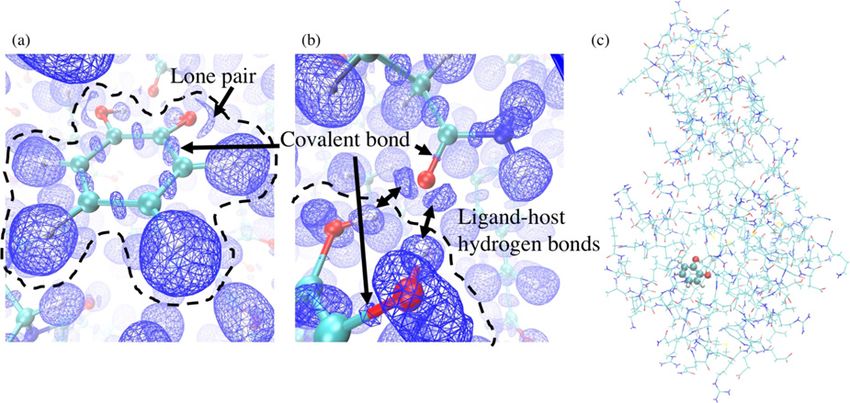
Electron. Struct. 2 (2020) 027001                                                             https://doi.org/10.1088/2516-1075/ab8d19

O P E N AC C E S S               TECHNICAL NOTE

                                 Electron localisation descriptors in ONETEP: a tool for
R E C E IVE D
3 January 2020
                                 interpreting localisation and bonding in large-scale DFT
R E VISE D
27 March 2020
                                 calculations
AC C E PTE D FOR PUBL IC ATION
24 April 2020                    R J Clements , J C Womack 1               and C-K Skylaris 2
PUBL ISHE D                      School of Chemistry, University of Southampton, Highfield, Southampton SO17 1BJ, United Kingdom
24 June 2020                     1
                                   Present address: School of Chemistry, University of Bristol, Cantock’s Close, Bristol, BS8 1TS, UK.
                                 2
                                   Author to whom any correspondence should be addressed.
Original content from            E-mail: C.Skylaris@soton.ac.uk
this work may be used
under the terms of the           Keywords: ONETEP, localised orbital locator, electron localisation function, density functional theory, linear scaling
Creative Commons
Attribution 4.0 licence.
                                 Supplementary material for this article is available online
Any further distribution
of this work must
maintain attribution to
the author(s) and the
title of the work, journal       Abstract
citation and DOI.                Electron localisation descriptors, such as the electron localisation function (ELF) and localised
                                 orbital locator (LOL) provide a visual tool for interpreting the results of electronic structure
                                 calculations. The descriptors produce a quantum valence shell electron pair repulsion (VSEPR)
                                 representation, indicating the localisation of electron pairs into bonding pairs and lone pairs in
                                 single molecules, coordination compounds and crystalline solids. We have implemented the ELF
                                 and LOL within ONETEP, a DFT code designed to perform calculations on systems containing
                                 thousands of atoms with plane-wave accuracy. This is possible using a linear-scaling formulation of
                                 DFT in which the Kohn–Sham orbitals are expressed in terms of a set of strictly localised
                                 non-orthogonal generalised Wannier functions (NGWFs), themselves expanded in a psinc basis
                                 set. In this paper, we describe our implementation and explore the chemical insights offered by
                                 electron localisation descriptors in ONETEP in a range of bonding and nonbonded
                                 situations.

                                 1. Introduction

                                 The electron localisation function (ELF) [1], devised by Edgecombe and Becke for Hartree–Fock (HF) cal-
                                 culations in 1990 and later extended to density functional theory (DFT) by Schmider and Becke in 2000
                                 [2], provides a useful tool for understanding chemical bonding from electronic structure calculations. The
                                 ELF indicates where pairs of electrons exist in the system, including lone pairs and bonding pairs. It is
                                 a dimensionless quantity, in the range of 0–1, with the purpose of providing a visual description of the
                                 chemical bond for almost all compounds [3]. The descriptor has been widely used over the years in the
                                 study of catalysis, organic synthesis, transition states and crystalline structures, for example [4–6]. The ELF
                                 is implemented in conventional DFT codes including CASTEP, Gaussian, Quantum Espresso and VASP
                                 [7–10].
                                     The ELF provides a valence shell electron pair repulsion (VSEPR) representation of coordination com-
                                 pounds. VSEPR is a simple model for understanding and interpreting electronic structure based on numbers
                                 of electron pairs, taught in many undergraduate chemistry courses [11]. σ and π bonds are distinguishable, as
                                 well as metallic and ionic bonding. The dimensionless quantity equals 1 in regions of perfect localisation with
                                 respect to a reference electron of like-spin. The ELF vanishes for one-electron regions dominated by a single,
                                 localised σ-spin orbital. The ELF corresponds to the electron gas-like pair probability when equal to 0.5. The
                                 quantity is a scalar field evaluable at all points in space, so can be visualised and interpreted alongside other
                                 similar quantities, for example electron density.

                                 © 2020 IOP Publishing Ltd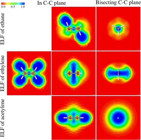
Electron. Struct. 2 (2020) 027001                                                                   R J Clements et al

    Here we describe the implementation of the ELF and a simpler version, the localised orbital locator (LOL)
[2], in ONETEP, which is a linear-scaling DFT code, with the aim of providing the capability for visual descrip-
tion of chemical bonding in larger systems than currently available, for example, protein–ligand complexes
involving a few thousand atoms. We present the reformulation of the ELF theory within the context of the
density matrix DFT implemented in ONETEP, in section 2, experimental details in section 3, and validation
using examples in section 4. This includes the results for single molecules and the key features of their covalent
bonds, bulk structures, and the directionality of nonbonded interactions in an entire protein–ligand complex
with ∼2600 atoms. We finish with some conclusions in section 5.

2. Theory and implementation

2.1. ONETEP
ONETEP [12], the order-N electronic total energy package, is a DFT code whose computational cost is
linear-scaling with respect to the number of atoms. The code uses a reformulation of the plane wave
pseudopotential method and retains the plane wave accuracy offered by conventional cubic-scaling DFT
codes.
    In ONETEP, non-orthogonal generalised Wannier functions (NGWFs) are used to expand the molecular
orbitals (MOs). The NGWFs are constrained to spherical localisation regions about the atom centres, to offer
a way of exploiting the locality of the density matrix, in order to achieve linear-scaling of calculations with
respect to system size. These NGWFs,

                                                     α
                                                     m∈L
                                          φα (r) =             D (r − rm ) cmα ,                                 (1)
                                                         m

are expanded in an orthogonal basis of periodic cardinal sinc (psinc) functions, D(r − rm ). Each psinc is cen-
tered on a point of a regular real-space Cartesian grid, rm . Only the psincs within the localisation region, Lα ,
are included, using a non-zero cmα [13, 14].
    A Fourier transform links psincs to plane waves, therefore, ONETEP ultimately runs calculations with
plane waves as with conventional plane wave pseudopotential DFT approaches, which allow for system-
atic improvement of the basis. Thus, the same control of accuracy is achieved, controlled just by the
grid spacing, which is specified via the kinetic energy cut off of the psinc functions. This accuracy has
been demonstrated by comparison against other non-linear-scaling codes such as CASTEP and NWChem
[15, 16].
    The NGWFs are optimised during the calculation rather than fixed, to allow for fewer local orbitals to be
used and to avoid transferability issues. This also has the important result of eliminating basis set superposition
error (BSSE) [17].
    The electronic density is constructed from the NGWFs as follows;

                                      nσ (r) = ρσ (r, r) = φασ (r)Kσαβ φ∗βσ (r),                                 (2)

using the Einstein summation for repeated Greek indices, for non-orthogonal quantities, where σ is the spin.
The density kernel, for spin σ,
                                                 N
                                                               †β
                                         Kσαβ =     M αiσ fiσ Miσ ,                                      (3)
                                                         i=1

where M is a linear transformation between the set of localised NGWFs, {φα (r)}, and the MOs, {ψ iσ (r)},
ψiσ (r) = φα (r)M αiσ . {fiσ } are the occupation numbers. In order to avoid cubic scaling steps, the {ψi }
and M are not calculated in practice, the calculation proceeds by calculating the NGWFs and the density
kernel.

2.2. Electron localisation function
The ELF was defined by Becke for HF and DFT and extended by Savin to periodic crystalline systems and
closed shell systems [1, 18], as follows:
                                                    1
                                          ELFσ =         ,                                        (4)
                                                 1 + χ2σ
for the individual spin, σ, where χσ (r) is the ratio,

                                                2(τσ (r) − τσW (r))   τσP (r)
                                     χσ (r) =         LSDA
                                                                    = LSDA    ,                                  (5)
                                                     τσ (r)          τσ (r)

                                                2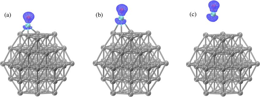
Electron. Struct. 2 (2020) 027001                                                                    R J Clements et al

τ σ (r) is the kinetic energy density,
                                                         1
                                                            N
                                              τσ (r) =       fiσ |∇ψσ (r)|2 .                                     (6)
                                                         2 i

τσW (r) is the von Weizsäcker approximation to the kinetic energy density,

                                                            1 |∇nσ (r)|2
                                                τσW (r) =                ,                                        (7)
                                                            8 nσ (r)
and where nσ (r) is the electronic density. The kinetic energy density for the uniform electron gas, τσLSDA (r),
named the local spin density approximation (LSDA), is
                                                                 5     5
                                                τσLSDA (r) = 2 3 cF nσ3 (r),                                      (8)
                                          2
where cF is the Fermi constant, 103 (3π 2 ) 3 .
    The numerator, τσP , contains all the electron localisation information. τσP will be small in regions of space,
r, where there is a high probability of finding a localised electron.
    To gain a physical interpretation, τσP is the difference between the kinetic energy density and the von
Weizsäcker kinetic energy density. τσW is the semi-local approximation to the kinetic energy density. The dif-
ference, τσP , therefore is excess kinetic energy density due to Pauli repulsion, which is called the Pauli kinetic
energy density. Also, the von Weizsäcker kinetic energy density is a lower bound to the positive definite orbital
kinetic energy density, in the limiting case where a single orbital is the main contributor to the density in that
region, at which point τ σ and τσW are equivalent, hence the Pauli kinetic energy density is always non-negative
[18–20].
    Pauli repulsion is lower in regions where electrons are less likely to encounter same-spin electrons, for
example, regions where electrons are more localised in covalent bonds or lone pairs. τσP is, therefore, small in
regions of high electron pair localisation. τσP ranges from arbitrarily small values, which give no indication of
how localised the electron is, to infinitely high values, therefore Becke and Edgecombe [1] proposed scaling
it with respect to the kinetic energy of the uniform electron gas, as shown in equation (5), and introduced
the mapping function (ELF) of equation (4). This formulation was chosen in order to obtain a more desirable
range of 0–1 for plotting, as opposed to having an open bound. Electron pair localisation can be found at
unity, i.e. when the probability of finding an electron in close proximity to another electron of the same spin
is zero.
    We have implemented the ELF in ONETEP using Becke’s definition with nσ (r) as the electronic density in
ONETEP, as defined above, in equation (2).
    The kinetic energy density has been implemented in ONETEP [21],
                                                             ⎛                   ⎞
                                           1
                                  τσ (r) =      (∇φασ (r)) · ⎝∇      Kσαβ φβσ (r)⎠ ,                            (9)
                                           2 α
                                                                           β

for overlapping NGWFs, φα and φβ , for each spin σ, and the density kernel Kσαβ as defined above.
    In the case of spin unpolarised systems, the up and down spin densities are equivalent to half of the total
electronic density; nσ = 12 n, therefore τσ = 12 τ and τσW = 12 τ W . χ, in terms of the total electronic density, is
therefore:
                                                  τσP (r)    2( 21 τ (r) − 12 τ W (r))
                                     χσ (r) =              =        5               5
                                                τσLSDA (r)        2 3 cF ( 12 n(r)) 3
                                                                2( 21 τ (r) − 12 τ W (r))
                                                            =      1  53 5       5
                                                                     2
                                                                          2 3 cF n 3 (r)
                                                                τ (r) − τ W (r)
                                                            =            5      .                                (10)
                                                                    cF n 3 (r)

    χσ is dimensionless, hence, the ELF is also dimensionless. For the case of the uniform electron gas, τσP and
τσLSDA are the same, therefore χσ equals 1; making the ELF equal to 0.5. This is a useful comparison value for
the analysis in the results and discussion section.

2.3. Localised orbital locator
We have also implemented the LOL, also introduced by Becke [2]. The LOL is similar to the ELF but is sim-
pler. Here, just the orbital kinetic energy density and the LSDA kinetic energy density are compared, without

                                                 3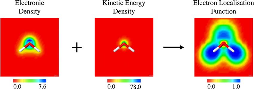
Electron. Struct. 2 (2020) 027001                                                                                         R J Clements et al

   Figure 1. The formulation of the ELF in terms of contour maps of the chemical components. The red green blue (RGB) colour
   scale ranges are given. The RGB scale for the ELF represents delocalisation to localisation, with respect to an electron of like-spin.
   Stick structures represent the molecules; oxygen is red and hydrogen is white.

considering the Pauli repulsion;
                                                                          1
                                                         LOLσ =               2τσ   .                                                  (11)
                                                                     1+
                                                                           τσLSDA

The quantity is, therefore, dimensionless for the LOL and ranges from 0–1 too, with localisation at unity.
   For the spin unpolarised case, like before we substitute in half of the total electronic density and half of the
kinetic energy density:
                                                           1
                                               LOL =             .                                            (12)
                                                       1+ τ5
                                                                           cF n 3

3. Calculation details

The ELF and the LOL were calculated for systems ranging in size, some of which were compared with the
original results of Edgecombe, Schmider and Becke, as well as additional analysis performed by Savin et al [3,
18, 20]. The XC functional rPBE was used for the nanoparticle systems, as used previously by Verga [22]. PBE
functionals were used for all other results. VMD version 1.9.4 [23] was used to plot the isosurfaces, and Jmol
version 14.29.24 [24] for the contour maps.
    An NGWF radius of 8.0 Bohr was used for every system, except for the Pt atoms of the nanoparticle and
the CO adsorbate, which had an NGWF radius of 9.0 Bohr. The kinetic energy cut off used was 900 eV for all
systems. A spherical Coulomb cut off of radius 28 Bohr was applied to the isolated hydrocarbons and 23 Bohr
to the water molecule. All systems were initially geometry relaxed using ONETEP.

4. Results and discussion

It is interesting to observe how the ELF compares with the ingredients that make it, the density and the kinetic
energy density. We show in figure 1 these three quantities as contour plots for the water molecule. These plots
clearly indicate the chemical information gained from calculating the ELF, while the density and kinetic energy
density are much less revealing in chemical terms. The regions of electron pairs are clearly shown in blue at
high values of the ELF. The lone pair can be identified above the oxygen, and the O–H bonding pair is also
clearly indicated.

4.1. Bonding types
The contour map of the ELF in figure 2 shows the covalent σ and π bonds in the molecules ethane, ethylene and
acetylene. Each type of C–C bond (single, double, triple) gives rise to a characteristic form of the ELF, which
enables the bonding type between the carbons to be identified without reference to the MOs. The π bond
is pictured as more of a ‘doughnut’ shape between the carbons, whereas the σ bond is oval. The π orbital is
more extended than the σ orbital. The region of the ELF that corresponds to the triple bond is much narrower
compared with the double bond, which seems to indicate that the ELF is not as intuitive in describing triple
bonds, possibly due to the delocalisation of the bonding electrons in two different planes. This is in agreement
with literature [3].
    The C–H bonds are represented by the diffuse blue regions surrounding the hydrogens in the contour
maps through the C–C and C–H plane. The atomic cores are coloured in red, representing no electron pair
localisation in the core region since we use norm-conserving pseudopotentials.

                                                        4
Electron. Struct. 2 (2020) 027001 R J Clements et al
Figure 2. Contour maps of the ELF in the plane and out of the plane of the molecules ethane, ethylene and acetylene. The RGB
colour scale ranges from 0 to 1. Stick structures represent the molecules; carbon is grey and hydrogen is white.
Figure 3. Contour maps of the ELF for (a) a 512-atom diamond cell in the 110 plane, (b) a 512-atom NaCl rocksalt structure in
the 110 plane and (c) a Pt55 -111 nanoparticle. Stick structures are only shown for bonds passing through the plane for clarity. The
RGB colour scale ranges are given. Relative scales are chosen to highlight the prominent features of each system.
4.2. Larger systems
To demonstrate the ELF calculated for larger systems, we tested two crystalline lattices; diamond and sodium
chloride. Figure 3 shows the ELF of these two in the 110-plane. The diamond lattice is comparable to results by
Savin et al [18]. The blue regions of high value indicate the shared pair of electrons of the C–C covalent bond.
The red centres on the carbons that match the value of the delocalised regions surrounding the molecules
are due to the norm-conserving pseudopotentials used. The core electron density is absent and the valence
electrons are not concentrated in this region. The NaCl lattice shows localisation solely on the atoms, as one
expects for ionic bonding, with no electron pairs between the atoms.
To test systems with metallic character, we use previous results from our group, by Verga et al, of CO adsorp-
tion onto a Pt nanoparticle in hollow (hcp) sites [22]. This is helpful for gaining insights to the uses of the
nanoparticle for catalytic activity, as these nanoparticles are models for catalysts. Electron localisation descrip-
tor (ELD) analysis here is helpful for gaining insights on electronic structure and the interactions between
reactants and surfaces. A cross section along the 111-plane through the Pt55 cuboctahedral nanoparticle is
shown in figure 3. Here the contour map demonstrates electron delocalisation between the atoms. There are
yellow–green valence regions on the Pt atoms, indicating that there is no electron localisation. The green–blue
surrounding regions do not correspond to the highly localised regions of covalent bonding between the atoms
seen in the diamond structure, but instead, these are continuous regions of relatively delocalised electrons
5Electron. Struct. 2 (2020) 027001 R J Clements et al
Figure 4. The ELF plotted as a blue mesh isosurface at 0.75 on a Pt55 -111 nanoparticle with CO adsorbed in a hollow (hcp) site.
(a) CO in a relaxed position, (b) and (c) CO shifted 1 and 2 Å away from the nanoparticle surface in the vertical direction,
respectively. Grey represents platinum, cyan carbon and red oxygen.
between the Pt atoms, indicated by a small ELF value of 0.4. This is clearly different from the red region between
the atoms of NaCl and between the carbon atoms of diamond where there is no electron pair presence. The
electron pair localisation only peaks at 0.44, for the Pt nanoparticle, which is not particularly high compared
with 0.93 of the covalent diamond and 0.88 of the ionic NaCl. This behaviour of the ELF is consistent with a
system with metallic character.
The ELF of the nanoparticle is also plotted as an isosurface in figure 4, at a value of 0.75. The first plot
is of the relaxed geometry of the Pt55 CO system. Going from left to right, the CO adsorbate is moved away
from the Pt surface in increments of 1 Å, in the vertical direction. First of all, looking at the Pt nanopar-
ticle, on the Pt atoms the ELF is negligible at a high localisation value of 0.75. This can be confirmed by
the contour plot in figure 3, the scale of which shows there are no regions taking this value. In contrast,
the ELF can be seen to show the delocalisation regions of the metallic nanoparticle as an isosurface in the
supplementary information (http://stacks.iop.org/EST/2/027001/mmedia), plotted at a much smaller value of
0.35.
Returning to the varying distance of CO from the Pt surface in figure 4, we observe a more well-defined
emergence of the lone pair on the carbon as the CO is moving away from the Pt, especially after a shift of 1 Å.
This is consistent with the disrupting of the σ-donor contribution of the CO as it is pulled away from Pt and is
returning to the isolated structure of the CO molecule. Equally observable is the strengthening of the bonding
between carbon and oxygen. This is further supported by contour plots of the CO in the supporting informa-
tion. The changes observed in the ELF as the Pt–CO distance increases are consistent with the conventional
picture of metal–carbonyl bonding.
4.3. Lone pair directionality in biomolecular interactions
Finally, we investigate the ELF on a system of biomolecular and pharmaceutical interest. This consists of the
interaction of a ligand with an entire protein (T4-lysozyme) with ∼2600 atoms, which we can calculate in
its entirety by using a linear-scaling code such as ONETEP. Here we perform calculations on one snapshot
of this complex from previous simulations by Fox et al [25], with the aim to examine what information
we can obtain from the ELF about the ligand–protein nonbonded interactions. For example, in figure 5,
where we focus on the region of the active site in the presence of the ligand, the ELF allows us to distin-
guish the presence of hydrogen bonds and lone pairs, which contribute to the protein–ligand stabilisation
interactions.
The visualisation of the ELF can also indicate directionality of the interactions. Here, the hydrogens of the
catechol ligand are pointing towards the oxygen electron pairs of the host protein, T4-lysozyme. The lone pairs
can also be seen on the oxygen of the catechol, as well as all of the bonding pairs in the carbon ring.
4.4. Linear-scaling computational effort
The key feature of ONETEP is its linear-scaling capability. In ONETEP, both the electronic density and kinetic
energy density, as given by equations (2) and (9), are quadratic forms, computed by the ‘FFT box’ technique, in
which Fourier transforms are applied to a subregion of the simulation cell, instead of the entire simulation cell
[12, 13]. Efficient algorithms have been developed to obtain these quantities, with similar procedures, except
that the evaluation of the kinetic energy density is more costly than the electronic density since it additionally
involves the application of the gradient operator and a scalar product over Cartesian components [21, 26]. As
discussed also in these previous papers, these quantities are nonzero only when the NGWFs α and β overlap
6Electron. Struct. 2 (2020) 027001 R J Clements et al
Figure 5. The ELF plotted as a blue mesh isosurface at 0.9 on a protein–ligand complex, T4-lysozyme with catechol. (a) The
ligand is central, contained within the broken line. (b) The ligand is in the bottom left corner. (c) The entire protein is represented
with lines and the ligand as a ball and stick structure for clarity. Carbons are cyan here, oxygen is red and nitrogen is blue.
Figure 6. Measured walltime for calculating the ELF as a function of the number of T4-lysozyme protein–catechol ligand
complexes (from 1 to 4) (black squares). The system was increased by one protein–ligand complex in the same direction, and the
simulation cell dimension was extended by its original dimension size used in the previous work of Fox et al [25], 154 Bohr, each
time. The (solid black) trendline, produced by the least squares method, shows a linear fit to the measured data. Calculations were
performed on the Iridis5 cluster using 16 nodes with 40 Intel Skylake cores each, running at 2.0 GHz, for a total of 64 MPI
processes, each spawning 10 OMP threads. Calculation parameters: kinetic energy cut off: 900 eV, NGWF localisation radius:
8.0a0 .
spatially. Given the localisation of the NGWFs, the number of these spatial overlaps is expected to increase
asymptotically linearly with respect to the system size. The implementation for the calculation of these quanti-
ties, in equations (2) and (9), is such that only the overlapping elements are included, and as a result, the overall
cost is expected to be linear-scaling. The ELF formula, in equation (4), is a local function of these quantities
so it is also expected to have a linear computational cost with the system size.
The calculation of the ELF was tested for its computational effort with respect to system size, for over
10 000 atoms, repeating the T4-lysozyme–catechol complex up to 4 times in an expanding simulation cell.
The results, in figure 6, demonstrate that the software does indeed achieve linear-scaling for the ELF cal-
culation, as the trendline of the measured data points is indeed linear. The linear-scaling cost of the total
energy calculation in ONETEP has been demonstrated elsewhere [12, 21]. In figure 6 the combined wall-
time for calculating the kinetic energy density, the electronic density and the construction of the ELF, is
plotted. This combined walltime is approximately 4% of the total walltime for the ONETEP properties
calculation.
4.5. LOL
The LOL [27], a simpler version of the ELF, has also been implemented in ONETEP. The only difference is that
in practice the values of the LOL range from 0 to only ∼0.6, as shown in the examples in the supplementary
information. From the examples given, the LOL can be regarded as producing slightly less chemically intuitive
contour plots, however the desirable features are still present.
7Electron. Struct. 2 (2020) 027001 R J Clements et al
5. Conclusions
We have presented the implementation of the electron localisation descriptors, the ELF and the LOL, in the
ONETEP linear-scaling DFT code. These descriptors provide a visualisation representation of electron pair
localisation in a system in terms of a scalar field, with values ranging from 0 to 1.
Importantly, the ELF is a visual descriptor and interpretative tool. We have compared our implementation
with other codes qualitatively, without the consideration of basis sets or any other fundamental differences
between codes. Our implementation of the ELF in ONETEP reproduces key qualitative features of other
implementations. We have demonstrated the chemical information that these descriptors provide using a
range of bonding situations, from isolated molecules to crystalline solids, with an example of how σ and
π bonding types can be distinguished using the ELF. We have presented examples on covalently bonded
materials such as diamond, ionic materials such NaCl, and metallic materials such as Pt nanoparticles. The
bonding between the atoms is distinctly different between these materials, and this is reflected in the ELF
representations. Furthermore, to demonstrate the usefulness of the ELF in biomolecular contexts, we have
presented an example of nonbonded interactions in a large protein–ligand complex, of interest to drug
design.
The availability of the ELF and LOL in a large-scale DFT code such as ONETEP opens the possibility for
providing additional chemical insight in a large range of applications, such as surface chemistry, reaction mech-
anisms, and drug design. Future extensions of these developments in ONETEP could include extension to PAW
calculations by including core densities and implementation of other visual electronic structures which make
use of the same quantities as the ELF.
The supplementary information contains further isosurface plots of the CO at varying distances from the
Pt55 nanoparticle and contour plots of these, with a comparison between the ELF and the LOL. Additionally
an isosurface of the LOL of the catechol ligand in the active site of T4-lysozyme is plotted.
Acknowledgments
RJC would like to thank the UKCP Consortium for funding a summer internship (Grant number:
EP/P022030/1) where the research started, also the Centre for Doctoral Training Next Generation of Com-
putational Modelling for a PhD studentship (Grant number: EP/L015382/1), and the resources of IRIDIS5
High Performance Computing Facility of the University of Southampton.
ORCID iDs
R J Clements https://orcid.org/0000-0003-4403-1258
J C Womack https://orcid.org/0000-0001-5497-4482
C-K Skylaris https://orcid.org/0000-0003-0258-3433
References
[1] Becke A D and Edgecombe K E 1990 A simple measure of electron localization in atomic and molecular systems J. Chem. Phys. 92
5397–403
[2] Becke A D and Schmider H L 2000 Chemical content of the kinetic energy density J. Mol. Struct.: THEOCHEM 527 51–61
[3] Savin A, Nesper R, Wengert S, Thomas F and Fässler E L F 1997 The electron localization function Angew. Chem., Int. Ed. Engl. 36
1808–32
[4] Dong F, Chaudret R, Piquemal J-P and Andrés Cisneros G 2013 Toward a deeper understanding of enzyme reactions using the
coupled ELF/NCI analysis: application to DNA repair enzymes J. Chem. Theory Comput. 9 2156–60
[5] Polo V, Andres J, Berski S, Domingo L R and Bernard S 2008 Understanding reaction mechanisms in organic chemistry from
catastrophe theory applied to the electron localization function topology J. Phys. Chem. A 112 7128–36
[6] Scheschkewitz D, Amii H, Gornitzka H, Schoeller W W, Bourissou D and Bertrand G 2002 Singlet diradicals: from transition
states to crystalline compounds Science 295 1880–1
[7] Clark S J, Segall M D, Pickard C J, Hasnip P J, Probert M J, Refson K and Payne M C 2005 First principles methods using CASTEP
Z. Kristallogr. 220 567–70
[8] Frisch M J et al 2016 Gaussian 16 Revision b.01 (Wallingford, CT: Gaussian Inc.)
[9] Amusia M Y, Msezane A Z and Shaginyan V R 2003 Density functional theory versus the Hartree–Fock method: comparative
assessment Phys. Scr. 68 C133–40
[10] Kresse G and Furthmüller J 1996 Efficient iterative schemes for ab initio total-energy calculations using a plane-wave basis set
Phys. Rev. B 54 11169–86
[11] Housecroft C E and Sharpe A G 2018 Inorganic Chemistry 5 edn (Harlow: Pearson)
[12] Skylaris C-K, Haynes P D, Mostofi A A and Payne M C 2005 Introducing ONETEP: linear-scaling density functional simulations
on parallel computers J. Chem. Phys. 122 084119
8Electron. Struct. 2 (2020) 027001 R J Clements et al
[13] Mostofi A A, Skylaris C-K, Haynes P D and Payne M C 2002 Total-energy calculations on a real space grid with localized functions
and a plane-wave basis Comput. Phys. Commun. 147 788–802
[14] Haynes P D, Skylaris C-K, Mostofi A A and Payne M C 2006 ONETEP: linear-scaling density-functional theory with local orbitals
and plane waves Phys. Status Solidi B 243 2489–99
[15] Fox S J, Pittock C, Fox T, Tautermann C S, Malcolm N and Skylaris C-K 2011 Electrostatic embedding in large-scale first
principles quantum mechanical calculations on biomolecules J. Chem. Phys. 135 224107
[16] Ruiz-Serrano Á L, Hine N D M and Skylaris C-K 2012 Pulay forces from localized orbitals optimized in situ using a psinc basis set
J. Chem. Phys. 136 234101
[17] Haynes P D, Skylaris C-K, Mostofi A A and Payne M C 2006 Elimination of basis set superposition error in linear-scaling
density-functional calculations with local orbitals optimised in situ Chem. Phys. Lett. 422 345–9
[18] Savin A, Jepsen O, Flad J, Andersen O K, Preuss H and von Schnering H G 1992 Electron localization in solid-state structures of
the elements: the diamond structure Angew. Chem., Int. Ed. Engl. 31 187–8
[19] Tal Y and Bader R F W 1978 Studies of the energy density functional approach I. Kinetic energy Int. J. Quantum Chem. 14 153–68
[20] Savin A, Silvi B and Colonna F 1996 Topological analysis of the electron localization function applied to delocalized bonds Can. J.
Chem. 74 1088–96
[21] Womack J C, Mardirossian N, Head-Gordon M and Skylaris C-K 2016 Self-consistent implementation of meta-GGA functionals
for the ONETEP linear-scaling electronic structure package J. Chem. Phys. 145 204114
[22] Verga L G, Russell A E and Skylaris C-K 2018 Ethanol, O, and CO adsorption on Pt nanoparticles: effects of nanoparticle size and
graphene support Phys. Chem. Chem. Phys. 20 25918–30
[23] Humphrey W, Dalke A and Schulten K 1996 VMD–visual molecular dynamics J. Mol. Graph. 14 33–8
[24] Jmol: an open-source Java viewer for chemical structures in 3D http://jmol.org/
[25] Dziedzic J, Fox S J, Fox T, Tautermann C S and Skylaris C-K 2012 Large-scale DFT calculations in implicit solvent—a case study
on the T4 lysozyme L99A/M102Q protein Int. J. Quantum Chem. 113 771–85
[26] Skylaris C-K, Haynes P D, Mostofi A A and Payne M C 2006 Implementation of linear-scaling plane wave density functional
theory on parallel computers Phys. Status Solidi B 243 973–88
[27] Schmider H L and Becke A D 2000 Chemical content of the kinetic energy density J. Mol. Struct.: THEOCHEM 527 51–61
9You can also read