Exiting from an Exchange Rate Floor in a Small Open Economy: Balance Sheet Implications of the Czech National Bank's Exchange Rate Commitment
←
→
Page content transcription
If your browser does not render page correctly, please read the page content below

Exiting from an Exchange Rate Floor in a
         Small Open Economy: Balance Sheet
       Implications of the Czech National Bank’s
             Exchange Rate Commitment∗

       Michal Franta,a Tomáš Holub,a,b and Branislav Saxaa
                            a
                                Czech National Bank
                                b
                                  Charles University

            The aim of this paper is to model the situation of a large
        central bank balance sheet with assets consisting almost exclu-
        sively of foreign exchange reserves in the circumstances of a
        catching-up economy exhibiting an exchange rate appreciation
        trend. As an illustration, we present projections of the Czech
        National Bank’s balance sheet after the discontinuation of its
        exchange rate commitment. Apart from the baseline projec-
        tion, which suggests a switch from losses to profits in 2026,
        several scenarios are discussed. Some relate to the exchange
        rate commitment itself (such as a discussion of its fiscal con-
        sequences), while others examine more general central bank
        balance sheet issues (such as a long-run decline in currency in
        circulation).
        JEL Codes: E52, E58, E47.

   ∗
    We would like to thank Kamil Galuščák, Dana Hájková, Michal Hlaváček,
Bernd Schlusche, Marek Šesták, Jan Vlček, Pierpaolo Benigno, and two refer-
ees at the IJCB, and seminar participants at the Slovak Economic Association
Meeting 2017 and at the Czech National Bank for valuable comments. We are
grateful to Adam Kučera for providing us with term premia estimates for USD
and EUR bonds, Martin Motl for sharing with us the data presented in Figure 2,
and Jaromı́r Tonner for counterfactual estimates of the macroeconomic variables
without the exchange rate floor. This work was supported by Czech National
Bank Research Project No. MP1/18. The opinions expressed in this paper are
those of the authors and not necessarily those of the Czech National Bank. Author
e-mails: michal.franta@cnb.cz; tomas.holub@cnb.cz; branislav.saxa@cnb.cz.

                                        51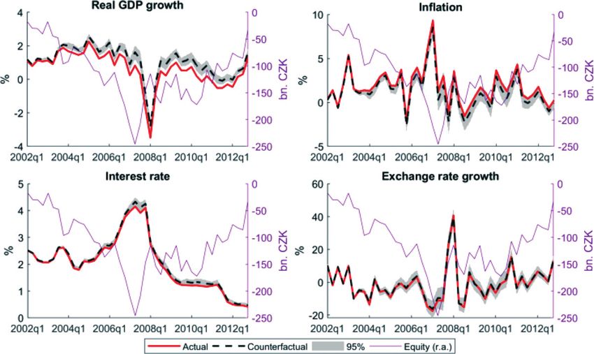
52         International Journal of Central Banking         June 2022

1.   Introduction

With the conduct of unconventional monetary policy after the global
financial crisis, central bank balance sheets have become a subject
of renewed interest. The issues of central bank solvency and fiscal
aspects of large balance sheets have received great attention from
researchers, who have focused, however, mainly on unconventional
monetary policies of major central banks such as the U.S. Federal
Reserve (the Fed) and the European Central Bank (ECB). They
have mostly concluded that the risk of central bank insolvency is
“real in theory, but remote in practice” (Hall and Reis 2015) or even
“truly negligible” (Cavallo et al. 2018). Nonetheless, it is impor-
tant to ask if such a conclusion also holds for a central bank with
assets consisting almost exclusively of foreign exchange reserves in
the circumstances of a small, open, catching-up economy exhibiting
an exchange rate appreciation trend.
    This paper therefore focuses on the central bank balance sheet
aspect of the Czech National Bank’s exchange rate commitment,
which was in place as an unconventional monetary policy instrument
from November 7, 2013 until April 6, 2017. When the commitment
was introduced, the Czech National Bank (CNB) made it clear that
its balance sheet consequences were seen as being of strictly sec-
ondary importance relative to the monetary policy objectives. The
central bank has also repeatedly emphasized that valuation losses on
its foreign currency portfolio induced by exchange rate appreciation
have no direct fiscal implications in terms of requiring a transfer
from the government budget, as the central bank will be able to
repay the losses out of its future profits, i.e., it remains solvent in
the long run.
    At the same time, the CNB’s exchange rate commitment may
have indirect fiscal implications in terms of reducing potential profit
transfers from the central bank to the government in the future.
There seems to be a relatively widespread belief in the Czech Repub-
lic outside the central bank that such indirect fiscal costs may be of
first-order importance and almost immediate. As a result, the CNB’s
balance sheet aspect will most probably remain a topic of public
debate for a protracted period of time. Indeed, after the exchange
rate commitment proved effective in terms of preventing deflation
and boosting the economic recovery (see Brůha and Tonner 2017)
Vol. 18 No. 2          Exiting from an Exchange Rate Floor            53

and was discontinued in a remarkably smooth manner, the main line
of criticism of this publicly unpopular policy shifted to the fiscal con-
sequences of the CNB’s valuation losses. These losses originate from
the devaluation of its massively larger foreign exchange reserves in
a situation of an appreciating exchange rate. Given the size of the
reserves and the long-term real equilibrium appreciation trend of the
Czech koruna, this phenomenon is likely to persist for an extended
period of time. It is necessary to be able to address this issue in a
quantitative analytical framework.
    Therefore, we develop and employ a simple balance sheet model
for a central bank of a small open economy with assets dominated by
foreign exchange reserves, and apply it to the CNB’s case.1 We show
how the model can be adjusted for different remittance policies and
thus employed by other central banks facing similar circumstances.
Next, we estimate balance sheet projections drawing on stochastic
simulations of the model. In addition to conveying a sense of the
uncertainty of the results, stochastic simulations enable probabilis-
tic assessment of various issues (such as the probability of negative
equity in a given year) and examination of questions that cannot
be examined in the deterministic setting (such as changes in the
composition of the foreign exchange (FX) reserves portfolio).
    In addition to the most probable balance sheet outlook, several
scenarios are discussed. Two of them are related to the exchange rate
commitment (the effect of the commitment on the balance sheet and
the simulation of an earlier exit from the commitment). Furthermore,
we demonstrate how some general balance sheet issues can be exam-
ined within the modeling framework—a long-run decline in currency
in circulation, sales of yields on FX reserves, and the relationship
between large negative equity and macroeconomic variables.
    We conclude that in the baseline scenario, the CNB can be
expected to stay in negative equity for about two decades, with a
trough roughly 10 years from now at around 6–7 percent of GDP.
This situation resembles the CNB’s previous experience with nega-
tive equity from 1998 until 2013, which did not lead to any solvency
issues or difficulties in pursuing appropriate policies. The financial or
“policy” solvency of the CNB is thus not endangered (even though

  1
    We extend an earlier approach of Cincibuch, Holub, and Hurnı́k (2009)
described in Appendix B.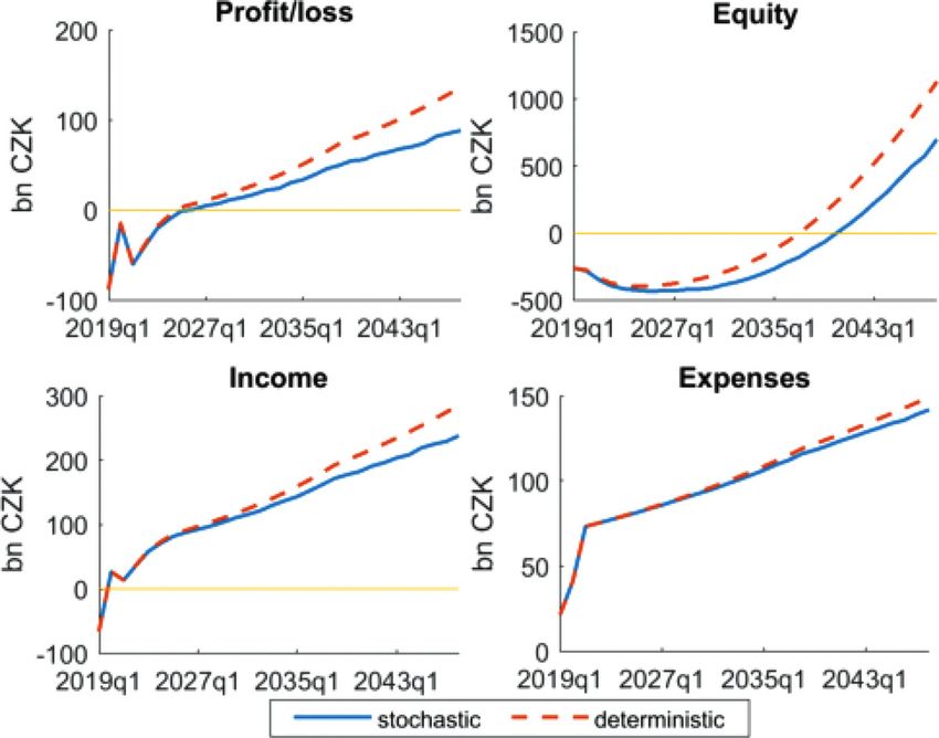
54          International Journal of Central Banking          June 2022

the uncertainty bands are very wide according to our stochastic sim-
ulations). At the same time, these findings may at first sight suggest
non-negligible indirect fiscal implications of the exchange rate com-
mitment. However, the counterfactual simulations of no exchange
rate commitment and earlier discontinuation of the commitment
show that the central bank’s equity would have stayed negative until
at least the year 2030 anyway. Given the institutional arrangements,
this means that there would probably have been no profit transfers
from the CNB to the Czech government in any case until that year.
From that point of view, the fiscal implications of the exchange rate
commitment related to the expansion of the central bank’s balance
sheet seem to be relatively small (especially if one also takes into
account the other indirect fiscal effects, which are clearly positive)
and fairly distant in time. This conclusion is relevant not just to
the CNB at present but in general to all small open economies with
central bank balance sheets dominated by foreign exchange reserves
that might consider using the exchange rate as an unconventional
monetary policy instrument in the future.
     Other scenarios suggest that a long-run decline in currency in cir-
culation can significantly affect the CNB’s balance sheet. However,
the main conclusion on the sustainability of central bank finances
still holds. Next, sales of yields on FX reserves do not affect the size
of the balance sheet too much but eliminate tail events represented
by prolonged periods of extremely negative equity. Finally, based on
the past Czech experience of negative equity, we found that taking
into account feedback effects between the CNB’s equity and macro-
economic variables implies a slightly less favorable outlook for the
balance sheet.
     The paper is organized as follows. In section 2 we summarize
key stylized facts associated with the balance sheet implications of
the CNB’s exchange rate commitment. Section 3 develops the bal-
ance sheet model. Section 4 provides stochastic simulations of future
CNB balance sheet developments. Section 5 uses the framework to
simulate several policy scenarios, bringing a quantitative dimension
to the recent public debates. Section 6 summarizes and concludes.
Appendix A presents the macro models applied in the stochastic sim-
ulations, while Appendix B compares our results with those based
on the Cincibuch, Holub, and Hurnı́k (2009) model. Appendix C
presents some additional results and Appendix D provides several
Vol. 18 No. 2         Exiting from an Exchange Rate Floor          55

notes on the asset-side composition. Finally, Appendix E discusses
various extensions of the baseline model for different remittance poli-
cies and for the Fed’s accounting treatment of losses in order to
compare it with the CNB’s approach.

2.   Stylized Facts on the Expansion and Composition
     of the CNB’s Balance Sheet

The CNB introduced its exchange rate commitment on November
7, 2013 in order to avoid deflation and to speed up the return of
inflation to the 2 percent target (Franta et al. 2014). To estab-
lish the exchange rate commitment and build its credibility, the
CNB had to purchase foreign exchange reserves worth EUR 7.5 bil-
lion (Figure 1) during the first few days of the commitment. For
the next 19 months, the exchange rate was above the exchange
rate “floor,” so the CNB did not have to intervene in the for-
eign exchange market. In this period, the foreign exchange reserves
were thus increasing only due to “client operations,” related mainly
to the drawdown of European Union (EU) funds. From mid-2015,
however, the exchange rate moved close to the announced “floor,”
influenced by the quantitative easing of the ECB and continued
favorable developments in the domestic economy. The CNB thus
had to start intervening whenever needed. The most pronounced
wave of interventions then took place in the first quarter of 2017.
By then, it was apparent that the exchange rate commitment was
coming to an end, and exporting companies were thus hedging
against possible future exchange rate appreciation. At the same time,
financial investors were building massive long positions in CZK.
The exchange rate commitment was discontinued on April 6, 2017,
once the CNB Board had concluded that the conditions had been
met for sustainable achievement of the 2 percent inflation target
in the future. Altogether, the FX interventions amounted to EUR
75.9 billion between November 2013 and April 2017 (another EUR
11 billion was purchased as part of client operations in the same
period). Since the exit, though, there have been no foreign exchange
interventions, as the exchange rate developments have been very
smooth.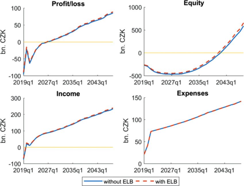
56            International Journal of Central Banking                 June 2022

          Figure 1. The CNB’s FX Operations during
               the Exchange Rate Commitment

Source: CNB.

    As a result, the CNB experienced a significant increase in its bal-
ance sheet size.2 Relative to GDP, its balance sheet expansion was
more significant than that of the U.S. Fed or the ECB. The most
significant difference compared with these two major central banks
arose in the first quarter of 2017, when the CNB’s foreign exchange
reserves jumped rapidly (Figure 2). Among other central banks, only
the Swiss National Bank (SNB) and the Bank of Japan have seen
bigger increases in their balance sheet size.3 Since the exit from the

    2
      Before 2013, the CNB’s balance sheet size relative to GDP had been declining
from its late-2002 peak, and later stagnating. This was partly due to a program
of selling income on the CNB’s FX reserves, which had been in place since 2004.
In November 2012, the CNB Board decided to suspend these sales, as the central
bank was getting ready for the potential use of the exchange rate as a mone-
tary policy instrument (see Franta et al. 2014). We discuss the balance sheet
consequences of the possible future resumption of this program in Section 5.4.
    3
      The Swiss case is similar to the Czech one in that the balance sheet increase
has been dominated by purchases of foreign exchange assets. At the same time,
though, the SNB has a very different institutional setup and tradition of profit
distribution than the CNB. The SNB has been a significant source of—rather
Vol. 18 No. 2            Exiting from an Exchange Rate Floor                 57

         Figure 2. The Central Bank’s Balance Sheet
              Size in International Comparison

Source: Bloomberg, CNB calculations.

exchange rate commitment, the CNB’s balance sheet has started to
decline gradually in relation to GDP. This reflects the absence of any
further foreign interventions, relatively swift nominal GDP growth,
and a decline in the CZK value of the FX reserves due to exchange
rate appreciation.
    As well as changing in size, the CNB’s balance sheet has changed
in composition, albeit less radically. This can be seen in Figure 3,
which compares the central bank’s balance sheet before the exchange
rate commitment (October 2013) with that immediately before the
exit (March 2017) and at the end of 2017. The asset side has
remained fully dominated by foreign assets, the bulk of which are
composed of the CNB’s foreign exchange reserves.4 The CNB’s other

stable—income not just for the Swiss federal government but also for local can-
tons. Its balance sheet developments have thus had important direct fiscal con-
sequences. As a result, Amador et al. (2016) argue that the concern about future
losses led to a “reverse speculative attack” and a forced exit from the SNB’s
exchange rate floor in early 2015. On the other hand, the CNB has paid (almost)
no dividend to the government since its inception in 1993, and was thus in a
better position to view its balance sheet expansion as a non-issue.
   4
     The FX reserves were already a dominant part of the CNB’s assets before
November 2013, reflecting (i) an inflow of foreign capital under the fixed exchange
rate regime that had been in place until May 1997, (ii) three waves of foreign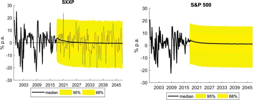
58            International Journal of Central Banking                  June 2022

               Figure 3. Composition of the CNB’s
                 Balance Sheet (in CZK billions)

Source: CNB.

assets are negligible. On the liability side, currency issued by the
CNB has continued to grow steadily, but most of the increase has
been concentrated in deposits of residents. These consist mainly
of commercial bank reserves placed at the CNB—which include
required reserves, two-week (henceforth 2W) repo operations,5 the
O/N (overnight) deposit facility, and free reserves—as well as gov-
ernment deposits at the central bank. Foreign currency liabilities
have increased, too, but to a much smaller extent than foreign

exchange interventions in the 1998–2002 period (see Geršl and Holub 2006), and
(iii) purchases of foreign currencies from the government, related initially mainly
to privatization revenues and later on to the drawdown of EU funds.
    5
      The Czech banking sector exhibits a systematic liquidity surplus. 2W repo
operations are thus used exclusively for absorbing liquidity, i.e., the CNB sells
securities to banks with a promise to buy the securities back two weeks later. That
is why the repo operations are listed on the liability side of the balance sheet and
they entail a corresponding decrease in reserve balances. A stylized central bank
balance sheet usually places net central bank operations on the asset side, because
in the majority of cases central bank operations provide liquidity. Note, however,
that the Federal Reserve balance sheet contains (reverse) repo agreements on
both the asset and the liability side.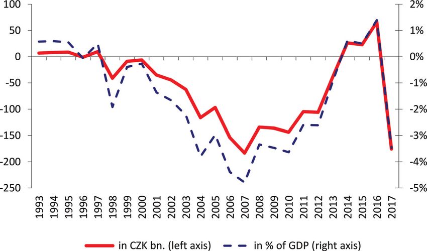
Vol. 18 No. 2           Exiting from an Exchange Rate Floor      59

                   Figure 4. The CNB’s Equity

Source: CNB, authors’ calculations.

currency assets, implying significantly increased exposure of the
CNB’s balance sheet to exchange rate changes. Compared with the
situation before the exchange rate commitment, a significantly larger
share of the liability side is now interest bearing, in contrast to
the interest-free currency that constitutes the base for the CNB’s
seigniorage (monetary income). The equity of the CNB was nega-
tive before the exchange rate commitment (at CZK –85 billion in
October 2013). It turned positive during the commitment period
(CZK 86 billion in March 2017), but has moved back into nega-
tive territory since then (CZK –172 billion at the end of 2017). The
CNB’s other liabilities have been very small.
    As can be seen in Figure 4, the CNB actually had negative
equity for 16 years before the exchange rate commitment was intro-
duced, from 1998 until 2013. It peaked at almost CZK –200 billion
in 2007, which at that time was equivalent to slightly less than 5
percent of annual GDP. In the late 1990s, the negative equity was
related to the cost of bank bail-outs, which were partly financed by
the central bank. Later on, the CNB’s losses originated from val-
uation losses associated with an appreciating trend of the koruna
against all major reserve currencies, given the dominance of for-
eign exchange reserves on the asset side of the CNB’s balance sheet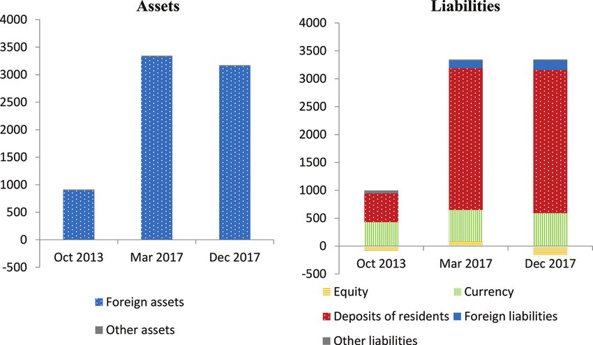
60            International Journal of Central Banking                    June 2022

and its mark-to-market approach to exchange rate changes (see Cin-
cibuch, Holub, and Hurnı́k 2009; Frait and Holub 2011). The CNB
followed a strategy of gradually repaying its accumulated losses out
of future profits, as it did not experience any negative impact of
negative equity on its policies (Benecká et al. 2012) or indepen-
dence. The accumulated losses were indeed fully repaid in 2014 (i.e.,
much earlier than suggested in Cincibuch, Holub, and Hurnı́k 2009)
thanks to depreciation of the koruna against the euro associated
with the exchange rate commitment and to even more pronounced
depreciation of the koruna against the U.S. dollar. The practically
zero sterilization costs during the episode of a technically zero inter-
est rate helped improve the CNB’s profitability, too. However, since
the exit from the CNB’s commitment, appreciation of the koruna
against the euro (by almost 6 percent) and the U.S. dollar (by 17
percent) have brought the central bank back into negative equity. At
the end of 2017, its size in absolute nominal terms broadly matched
the pre-crisis peak of 2007. Relative to GDP, it was slightly smaller
due to a higher level of domestic economic activity in nominal terms.
    Given the structure of its balance sheet presented in Figure 3, the
CNB’s financial results are predominantly affected by two factors.
First, they reflect the returns on foreign exchange reserves expressed
in CZK, which consist of the yields in foreign currencies and the
valuation effects stemming from changes in the value of the Czech
koruna against a basket of reserve currencies. Exchange rate changes
and capital gains or losses on assets in the CNB’s reserves portfolio
are both marked-to-market and thus immediately affect the central
bank’s equity.6 Second, the interest rates paid on the deposits of res-
idents at the CNB—mainly remunerated at the 2W repo rate—are
the main item on the costs side. As can be seen in Figure 5, the

    6
      Exchange rate gains and losses enter the CNB’s profit and loss account and
thus also its equity. The same is true for all realized capital gains or losses on
assets in the FX reserves portfolio, as well as for any unrealized gains and losses in
its stock indexes part. In the past (until 2018), unrealized capital gains or losses
on fixed-income assets (bonds) were not shown in the profit and loss account,
but instead were put into a revaluation reserve, which, however, is a part of the
CNB’s equity, too. For more information on the CNB’s accounting procedures,
see CNB (2018). In our simulations, we abstract from the distinction between
realized and unrealized gains on bonds.
Vol. 18 No. 2 Exiting from an Exchange Rate Floor 61
Figure 5. The CNB’s Sterilization
Costs and Yields on FX Reserves
Source: CNB.
yields on the CNB’s FX reserves in foreign currencies have consis-
tently exceeded the 2W repo rate in the last 10–15 years. However,
exchange rate changes have often dominated in terms of CZK yields
and thus the overall profit and loss account of the CNB.
Looking into the future, the two key questions for the CNB’s
ability to repay its current accumulated loss are thus (i) whether
the positive differential between the foreign currency yield on the
FX reserves and the 2W repo rate remains in place (especially as
the CNB has started to normalize its monetary policy well ahead
of the ECB) and (ii) if the nominal currency appreciation is smaller
or larger than this differential on average. The answer to the former
question partly depends on how the CNB’s foreign exchange reserves
are managed regarding the risk-return trade-off. The latter question
is related to the future pace of convergence of the Czech economy
to the advanced countries.
The repayment of accumulated losses will—as in the past
episode—be facilitated by favorable institutional arrangements
related to the CNB’s profit distribution. Income losses are absorbed
by corresponding variations in the equity position. Specifically, when
the CNB incurs an operating loss, that loss is absorbed through a62 International Journal of Central Banking June 2022
decrease in the CNB’s equity position of equal size.7 And, at the
end of the subsequent fiscal year, even if the CNB makes a profit,
this does not necessarily imply that it will resume its remittances
(transfers) to the fiscal authority. Such an outcome, in fact, depends
in the first place on the CNB’s equity position. If this position is neg-
ative, remittances cannot resume until the CNB has made enough
profits to make it less negative and ultimately bring it back into the
non-negative domain. Even then, that is, when the equity position is
no longer negative, the CNB can choose, at its discretion, to retain
at least part, if not all, of its positive income realizations to further
build up its stock of assets, thereby lowering the potential for future
losses.
It is important to bear in mind this arrangement when drawing
conclusions about the potential fiscal consequences of the various
policies simulated in the subsequent part of this paper. In partic-
ular, the crucial outcome is the duration of the negative equity in
various scenarios rather than the size of the negative equity in any
particular year or at its peak. This is because the government gets
no profit transfer no matter how large the negative equity is. At
the same time, the year when the CNB’s accounting equity returns
above zero must be viewed as the earliest possible date of start-
ing profit transfers, although this does not mean they would start
automatically.
3. Model of the Czech National Bank’s Balance Sheet
In this section we develop a model for analyzing balance sheet issues
for a CNB-like central bank that employs the fair-value accounting
approach.8 The following equations assume a simplified structure
of the CNB’s balance sheet, with assets comprising foreign assets
only and liabilities encompassing currency in circulation, deposits
7
Note that the government has no obligation to recapitalize the central bank.
8
As concisely defined, for example, in Bonis, Fiesthumel, and Noonan (2018),
fair value “represents the market price that would be received in selling an asset
in an orderly transaction between market participants at the measurement date,
which is the date reported in the financial statements.” The fair-value account-
ing approach means that the income and capital position of the central bank are
affected by changes in the market value of a security.Vol. 18 No. 2 Exiting from an Exchange Rate Floor 63
of residents (predominantly banks and to a lesser extent the gov-
ernment), and equity. These are the dominant components of the
CNB’s balance sheet (see above in Section 2).9
Income in year t, Inct , comprises the yield on holdings of foreign
assets at the end of the previous year, F Xt−1 , which are assumed
to be denominated in euros (70 percent) and U.S. dollars (30 per-
cent). The effective yield on foreign assets expressed in the domestic
currency is the weighted sum of the foreign portfolio yields and the
appreciation/depreciation of the koruna with respect to the euro and
the dollar:10
Inct = 0.7 yieldEU
t
R
+ ΔeEU
t
R
F Xt−1
U SD U SD
+ 0.3 yieldt + Δet F Xt−1 . (1)
For both euro- and U.S.-dollar-denominated assets, we assume that
90 percent of the assets will yield a return equal to the expected
yield on one-year bonds,11 while the remaining 10 percent of the
assets are invested in a stock portfolio.
The next year’s foreign assets increase by current-year income.12
Moreover, we add the possibility of autonomous changes in FX hold-
ings made by the central bank during year t, F XIntt . Such transac-
tions could include FX interventions, EU fund purchases, and sales
9
To make the observed values of the balance sheet items numerically consis-
tent, we distribute all other non-zero items into the three dominant categories.
External liabilities are added with a minus sign to foreign assets, and all other
items (remaining liabilities, loans to residents, fixed assets, and remaining assets)
are added with the relevant sign to deposits of residents.
10
The equation employed for income is an approximation.
For a given for-
Et+1
eign currency, income equals Et
(1 + yieldt ) − 1 F X t−1 , where Et denotes
the nominal exchange rate at the beginning of period t. Standard logarithmic
approximation then implies the formula for income.
11
At the end of 2017, the durations of the EUR and USD investment tranches
were 2.7 and 5 years, respectively. The durations of the liquidity tranches were
approximately 0.1 year in both the EUR and USD portfolios.
12
The current-year income is invested in foreign currency assets. This assump-
tion is relaxed in Section 5.4. Next, we implicitly assume that the FX portfolio
is reinvested each period in order to maintain the assumed composition in terms
of both currency and bonds and stocks. Several notes concerning the stock-bond
ratio can be found in Appendix D.64 International Journal of Central Banking June 2022
of income on FX reserves. Including this term allows the model to
be used to conduct various policy-relevant simulations.
F Xt = F Xt−1 + Inct + F XIntt (2)
The expenses of the CNB, Expt , include interest payments on the
deposits of residents. We assume that the interest rate applied is
equal to the main policy rate, i.e., the two-week repo rate paid on
the CNB’s main monetary policy facility.13 Operational costs, OCt ,
are included and are assumed to be a constant fraction of nomi-
nal GDP, specifically the average fraction observed over the period
2006–15.
Expt = iCZ
t Dept−1 + OCt (3)
Overall liabilities evolve according to the standard law of motion
extended to include the possibility of direct FX transactions by the
bank, which is reflected by the liability side, and possible transfers
from the central bank to government:
Liabt = Liabt−1 + Expt + F XIntt + T rt . (4)
The term T rt represents a discretionary outlay due to the CNB’s
remittance policy described in Section 2. The only constraints on
profit transfers imposed by law are the following:
T rt = 0 if Eqt ≤ 0 or Πt ≤ 0
(5)
0 ≤ T r t ≤ Πt otherwise,
where Eqt stands for the central bank’s equity at the end of period
t. In the case of positive transfers, the account that the government
holds with the central bank is credited with the transferred amount
and the central bank’s equity is reduced correspondingly through an
increase of liabilities14
13
Domestic banks can deposit their excess liquidity at the CNB for a two-week
period on the basis of repurchase agreements (“repos”) at a rate not exceeding—
but typically very close to—the two-week repo rate.
14
In the following benchmark simulations and simulations underlying all the
scenarios, profit transfers are assumed to be zero. The main reason for this is the
historical experience with a long period of zero transfers covering periods withVol. 18 No. 2 Exiting from an Exchange Rate Floor 65
Deposits are calculated as the residual of total liabilities and
currency in circulation (Casht ):
Dept = Liabt − Casht , (6)
where the growth rate of currency in circulation is approximated by
nominal GDP growth gt :15
Casht = (1 + gt ) Casht−1 . (7)
The profit or loss (net income) of the central bank is defined as the
difference between income and expenses. Equity is then defined as
the difference between central bank assets and liabilities; its current
level reflects equity in the previous year adjusted for the profit or
loss and possible profit transfer to government):
Πt = Inct − Expt (8)
Eqt ≡ F Xt − Liabt
= F Xt−1 + Inct + F XIntt
(9)
− (Liabt−1 + Expt + F XIntt + T rt )
= Eqt−1 + Πt − T rt .
The balance sheet model (1)–(9) can be easily adjusted for different
remittance policies, and we discuss such extensions for the cases of
the Swiss National Bank, the Riksbank, and the Bank of Korea in
Appendix E. In addition, the case of the Federal Reserve is touched
upon in this appendix.
Given the accounting equations (1)–(9), the projections of the
balance sheet items and the income statement are based on the
both negative and positive equity. So, it is reasonable to apply the same approach
to transfers in the future. Importantly, the median equity, which is of primary
interest, is negative in the benchmark and the scenarios for the vast majority of
periods and so is not affected by changes in positive parts of the simulated equity
paths brought about by potential transfers to government. Therefore, the median
is intact after imposing non-zero profit transfers for positive equity paths in the
simulation. That is why our assumption of zero transfers is not crucial. Non-zero
transfers are discussed in Appendix E.
15
An alternative to the usual assumption of currency growth equal to nominal
GDP growth is to model money demand explicitly, as in Veracierto (2018).66 International Journal of Central Banking June 2022
macroeconomic forecast officially published by the CNB,16 the equi-
librium values employed in the CNB’s forecasting process, and the
outlooks for financial variables taken from yield curves and historical
averages of stock returns.
The macroeconomic outlook for the domestic monetary policy
rate, nominal output, and exchange rates for the first two years of
the projection is taken from the official CNB forecast. The outlook
beyond two years ahead is approximated using the equilibrium val-
ues (Table 1, first row). They converge linearly to the equilibrium
values expected at the end of the convergence process (Table 1, sec-
ond row), which is assumed to occur after 20 years. The termination
of the convergence process resembles the situation of euro-area entry,
because in such a situation the foreign monetary policy interest rate
becomes the domestic rate and the exchange rate with respect to
the euro can be viewed as fixed. So, we can reasonably interpret the
situation after 20 years in both ways.17
The expected yield on the one-year euro bond used to approxi-
mate the euro bond portfolio yield is based on the 3M EURIBOR
(three-month euro-area interbank offered rate) outlook from the
CNB’s forecast adjusted for the spread between the three-month
rate and the one-year rate for the first six years of simulations.18
The expected yield on the one-year U.S. Treasury bond is based
on the observed financial market yield curve and estimates of the
term premia for the first 10 years of simulations.19 After 6 and 10
years, the expected yields for both the euro and dollar bond portfo-
lios converge to the equilibrium value, calculated as the equilibrium
value of the 3M EURIBOR assumed in the CNB forecasting process
16
The forecast published in Inflation Report I/2018.
17
We do not, however, take into account that euro adoption would imply CNB
participation in the redistribution of monetary income among euro-area central
banks. This issue was analyzed in Cincibuch, Holub, and Hurnı́k (2008).
18
ECB (2017) provides estimates of 10-year term premia that are slightly higher
than the term premium implied by the compounded 1-year EUR interest rate out-
look applied in the CNB forecast and the observed yield curve. We therefore view
the EUR interest rate outlook based on the CNB forecast as reasonable.
19
The USD portfolio forward rate is calculated using the yield curve
and term premia estimates from the no-arbitrage term structure model
described in Adrian, Crump, and Moench (2013). The data are available
at http://libertystreeteconomics.newyorkfed.org/2014/05/treasury-term-premia-
1961-present.html.Vol. 18 No. 2
Table 1. Equilibrium Values
3M CZK/ CZK/
Portfolio
PRIBOR – Currency in EUR USD
Return
3M 2W Repo Circulation yoy yoy 3M
PRIBOR Spread Inflation Growth Rate Change Change EURIBOR EUR USD
CNB Forecast 3.00 0.24 2.00 5.00 −1.50 −1.50 3.50 — —
End of Convergence 3.50 0.24 2.00 3.00 0.00 0.00 3.50 4.02 4.02
(or Euro Zone Entry)
Exiting from an Exchange Rate Floor
6768 International Journal of Central Banking June 2022
increased by the average difference between the three-month rate
and the one-year euro bond yield.20 The equilibrium yield is assumed
starting with the twentieth year of the outlook. The expected yield
on the stock portfolio is approximated by the average historical stock
market yields in the respective currencies over the whole projection
horizon. For both the EUR and USD market, the value is set to 6
percent per annum.21
To obtain stochastic projections of the CNB’s income statement
and balance sheet items, we follow the methodology employed in
Ferris, Soo, and Schlusche (2017). As a starting point, the deter-
ministic path defined above is taken. Then 10,000 forecast paths
of the macroeconomic variables around the deterministic path are
generated.22 The forecast paths reflect the size of the shocks and
their effects estimated on historical data. The core model used to
generate the set of paths is a small-scale Bayesian vector autore-
gression (BVAR) one tailored to the Czech economy. In addition,
simple satellite models are employed to generate forecast paths
for stock returns and CZK/USD appreciation/depreciation. The
accuracy of the underlying macro models is crucial for the accu-
racy of the stochastic projections of the balance sheet. Therefore,
details of the models and some additional results are presented in
Appendix A.
4. Benchmark Simulation
The simulation is based on the values of the balance sheet items as of
December 31, 2017 and the CNB’s official macroeconomic forecast
published in Inflation Report I/2018, i.e., the forecast that starts
with 2018 as the first forecasted year. The simulations are at yearly
20
The average difference between the 3M EURIBOR and the one-year euro
bond yield is computed over the periods 2004:Q1–2007:Q4 and 2009:Q1–2017:Q4,
i.e., with the exception of 2008, when the spreads reflected a money market freeze.
The spread equals 0.3 percentage point.
21
In reality, this yield will be time varying and negatively correlated with the
government bond yield. This negative correlation was in fact the main reason
for adding the equities to the CNB’s reserve portfolio. It is implemented in the
stochastic simulations presented in Section 4 via the variance-covariance matrix
of annual yields.
22
To check whether 10,000 draws is a sufficient number, a robustness exercise
with 2,500 draws only is performed, yielding very similar results.Vol. 18 No. 2 Exiting from an Exchange Rate Floor 69
Figure 6. CNB Balance Sheet Outlook (baseline scenario)
Note: The “closest-to-median path” is the forecast path closest to the pointwise
medians of all four simulated quantities (see footnote 23).
frequency. The first simulated values relate to the first quarter of
2019, i.e., flows represent the period 2018:Q1–2018:Q4 and stock
variables pertain to the first day of 2019. The projection period
covers 30 years.
Figure 6 shows the baseline simulation of the CNB income state-
ment outlook together with the evolution of equity.23 The presented
quantities are in nominal terms. The uncertainty around the median
23
Note that the median profit is not necessarily equal to the difference between
the median income and the median expenses, because the forecast paths under-
lying the three medians can differ. For a given forecast path, the equality holds.
The solution could be to take the forecast path that implies the closest-to-median
profit, income, and expenses and work with that path. Such path is shown in
Figure 6, which suggests that no additional information on the dynamics of the
system in general is provided by using the closest-to-median paths instead of the
pointwise median paths. We therefore stick to the standard approach and present
pointwise medians in the paper.70 International Journal of Central Banking June 2022
projections expressed by the 68 percent and 95 percent of the dis-
tributions is substantial and grows with the length of the projection
horizon. Moreover, the simulated distributions are skewed. While
the macroeconomic outlooks are symmetric around the determinis-
tic path, the implied distributions of income statement items and
equity are asymmetric, because the balance sheet accounting iden-
tities are non-linear. For example, assuming constant interest rate
and exchange rate outlooks, income becomes an exponential func-
tion of time with parameters determined by the two outlooks. The
normally distributed interest rate and exchange rate are then trans-
formed into a log-normally distributed income distribution, which
is skewed. The sign of the skewness is determined by the particu-
lar assumed values of the macroeconomic variables constituting the
deterministic path.
The wide range of uncertainty can be illustrated on past experi-
ence using deterministic simulations based on Cincibuch, Holub, and
Hurnı́k (2009) at the CNB. While this model initially—in the phase
of fast convergence and exchange rate appreciation—significantly
underestimated the extent of the CNB’s losses and negative equity,
the situation changed abruptly with the unexpected major shock
generated by the global crisis. This led to much faster elimination
of the CNB’s negative equity compared with the simulations, fol-
lowed by rapid reemergence of the losses once the central bank dis-
continued its exchange rate commitment in 2017 (and the dollar
simultaneously started to depreciate against the euro). In general,
the financial outcome and equity of a central bank with the CNB’s
balance sheet size and structure can be strongly countercyclical; it
tends to improve in adverse situations with a depreciating currency
and deteriorate in cyclical upswings with an appreciating currency.
But given that the deterministic simulations draw their macroeco-
nomic assumptions from sources that are by definition not able to
forecast major future cyclical swings, the uncertainty around them
is huge.
To assess the evolution of balance sheet items from the point
of view of their sustainability, the ratios of total assets to nominal
GDP and equity to GDP can be simulated. This is done in Figure 7,
which shows (in the left panel) that the median projection of the
ratio of total assets to GDP is located below 0.5 for the whole 30
years with the exception of the first year. The probability that theVol. 18 No. 2 Exiting from an Exchange Rate Floor 71
Figure 7. Projections of the Ratios of Total
Assets to GDP and Equity to GDP
size of the balance sheet exceeds that of GDP—defined as the ratio of
the simulated balance sheets with this property to all the simulated
balance sheets—starts at zero and reaches 0.03 at the end of the
projection horizon. Only two central banks of advanced economies
currently exhibit a ratio exceeding 0.5—the Bank of Japan and the
Swiss National Bank. Regarding the expected ratio of equity to GDP,
Figure 7 (right panel) suggests that the median never falls below
–8 percent of GDP. The probability of negative equity starts at
0.91 and 0.82 in 2018 and 2019, respectively, and decreases steadily
towards 0.43 in 30 years.
To obtain a more focused picture, Figure 8 presents the medians
of the benchmark stochastic projections (with all the above reserva-
tions concerning the reliability of the projections in mind). It turns
out that the loss will be highest in the first year of the projection at
approximately CZK 88 billion, which is equivalent to 1.6 percent of
the GDP forecasted for that period. The loss will then diminish and
turn into a profit after eight years in 2026. As a consequence, the
equity will be negative for roughly the next two decades, the lowest
point being negative equity of CZK 458 billion (i.e., 6.6 percent of
GDP) in 2027:Q1. Appendix B shows that these results are quali-
tatively similar to the outcomes of the earlier model of Cincibuch,
Holub, and Hurnı́k (2009) but are somewhat more optimistic overall
in the longer term given our more nuanced approximation of future
yields on the CNB’s foreign exchange reserves.
From the historical perspective, the negative equity expected
during the coming 23 years is not so far from the CNB’s past72 International Journal of Central Banking June 2022
Figure 8. CNB Balance Sheet Outlook (medians)
experience of negative equity lasting 16 years over the period 1998
to 2013 (see Section 2). Moreover, without the exchange rate com-
mitment, the span of the period of negative equity starting at the
end of the 1990s would have been longer (see Section 5.1 below). In
terms of the size of the accumulated loss, the near future is close
to the situation the CNB faced in 2007, when its negative equity
approached 5 percent of GDP.
5. Policy Scenarios
Several policy scenarios are discussed in this section. The aim of the
first two is to contribute to the public debate that has arisen around
the central bank balance sheet recently in the Czech Republic. The
debate revolves around the fiscal consequences of the exchange rate
commitment, based on the idea that with a different past monetary
policy the CNB would soon have been able to start paying dividends
to the Czech government.24 We provide a quantitative assessment of
24
In reality, the CNB has never paid a dividend to the government since it was
established in 1993 (with one negligible exception). The debate is thus in itself
very hypothetical.Vol. 18 No. 2 Exiting from an Exchange Rate Floor 73
this idea, something which has so far not been delivered by its propo-
nents. The third and fourth scenarios address the possible long-run
decline in the amount of currency in circulation and the scope for
active management of the central bank’s balance sheet by means of
resuming the program of selling yields on the FX reserves. Finally,
the last scenario discusses the relationship between the CNB’s large
negative equity and inflation.
5.1 Counterfactual Scenario of No
Exchange Rate Commitment
The first scenario considers the situation of no exchange rate com-
mitment. The use of the exchange rate as an additional mone-
tary policy tool was introduced in November 2013 and discon-
tinued in April 2017. The scenario works with the balance sheet
items as of October 31, 2013, i.e., without the central bank’s pur-
chases of euros related to the floor. The counterfactual estimates of
GDP growth, the domestic interest rate, and the CZK/EUR and
CZK/USD exchange rates are taken from Brůha and Tonner (2017)
based on the dynamic stochastic general equilibrium (DSGE) model
with the labor market block described in Tonner, Tvrz, and Vasicek
(2015). The estimates of the evolution of domestic variables with-
out the floor are available for the period 2013:Q4–2015:Q4. For the
following years we assume a transition to the steady state similarly
to the benchmark case. We therefore abstract from the observed
shocks that apparently hit the economy in 2016 and 2017. For for-
eign variables (EUR and USD interest rates), the observed values
are taken for the first four years of the counterfactual projection
and the outlooks are based on the most recent market expectations
afterwards.25
Figure 9 shows that without the exchange rate commitment, the
CNB’s equity in the first three years would have been lower than the
25
Note that the counterfactual scenario is based on a model where endoge-
nous variables reach steady state sooner or later and where economic agents with
rational expectations consider the inflation target as fully credible. In reality, one
of the motivations for the introduction of the exchange rate commitment was
the risk of the deflationary spiral where expectations become unanchored on the
inflation target. Such scenario would lead to much more adverse developments of
the Czech economy than the counterfactual scenario considers.74 International Journal of Central Banking June 2022
Figure 9. No Exchange Rate Commitment
Note: The benchmark simulation (exchange rate (ER) commitment) is computed
starting with 2017:Q4–2018:Q3 to follow the timing of the no-ER-commitment
scenario. The original benchmark simulation started with 2018:Q1–2018:Q4.
observed actual numbers (see asterisks in this figure). This is due to
lower GDP (and currency) growth and especially due to a stronger
currency in the counterfactual scenario without the commitment,
which implies a lower value of FX reserves expressed in the domes-
tic currency and thus lower equity.26 Subsequently, the size of the
negative equity would have been less than half that in the bench-
mark simulation due to a lower stock of foreign exchange reserves
and the resulting less-adverse valuation losses (in combination with
the assumption of no deflation spiral in the counterfactual scenario
and neutrality of monetary policy for long-term real economic devel-
opments). The time span of negative equity, however, would be 18
years from the beginning of the simulation. Interestingly, this is not
much less than in the benchmark case with the exchange rate com-
mitment, where negative equity is projected for 23 years (although
starting in 2017/2018). In terms of the CNB’s (in-)ability to pay
dividends to the government, the counterfactual simulation is thus
no more optimistic than the benchmark until around 2030. This
shows the importance of quantifying the counterfactual scenario if
26
Note that the CNB’s FX reserves were smaller but still substantial before
the exchange rate commitment was introduced (see Section 2).Vol. 18 No. 2 Exiting from an Exchange Rate Floor 75
one wants to discuss the fiscal consequences of the CNB’s exchange
rate commitment in depth.27
5.2 Hypothetical Termination of the Exchange
Rate Commitment at the End of 2016
The second policy scenario concerns the question of how the balance
sheet and its outlook would have looked if the exchange rate com-
mitment had been terminated at the end of 2016. This situation is a
subject of local public debate. The popular argument goes that an
earlier exit at the end of 2016 would have led to a much smaller bal-
ance sheet and consequently to an earlier potential transfer of profits
to the Ministry of Finance. The extension of the CNB’s exchange
rate commitment into 2017 is thus criticized for having had major
(and—implicitly presumed—almost immediate) fiscal implications.
There are two major flaws to this argument. First, in September
2016 the CNB committed not to “discontinue the use of the exchange
rate as a monetary policy instrument before 2017 Q2” (CNB 2016).
It is extremely unrealistic to assume that the increase in the CNB’s
FX reserves in November and December 2016 would have been the
same as the one observed in reality without this extended commit-
ment. Most probably, exporters would have hedged before the end of
2016, and financial investors would have done the same as regards
building their long CZK speculative positions. There is no signif-
icant reason to believe that the overall size of the CNB’s balance
sheet expansion would have been much lower; it would just have
had a different timing. The only way to avoid the observed balance
sheet increase would probably have been to extend the “hard” com-
mitment in autumn 2016 and then break it. However, this would
27
Moreover, when assessing the overall fiscal consequences of the exchange
rate commitment, one cannot just look at the CNB’s equity and potential future
transfers of profits from the central bank to the government. In the hypothetical
scenario without the commitment, the lower nominal GDP growth would lead
mainly to a deterioration in the primary government budget balance as a result
of lower revenues, and to an adverse denominator effect. In addition, the higher
interest rate would increase the costs of debt service. Using the “no exchange rate
commitment” counterfactual scenario in Brůha and Tonner (2017), the CNB’s fis-
cal experts have estimated the debt/GDP ratio as reaching 42.7 percent at the
end of 2015 in the hypothetical scenario without the commitment, compared with
the observed 40 percent level.76 International Journal of Central Banking June 2022
Figure 10. Early Exit from the Exchange
Rate Commitment (medians)
have been extremely harmful to the CNB’s credibility. At the same
time, the exchange rate developments after such a surprising exit
would probably have been much less smooth than in reality; and
with a more pronounced CZK appreciation, the CNB’s equity might
have turned more negative even with a smaller balance sheet.
Second, even if one ignores the above fundamental issues, none
of the CNB’s critics have taken the trouble to quantify the impli-
cations of a smaller central bank balance sheet. In Figure 10, we
thus provide a simulation with the—extremely unlikely—assumption
that the CNB’s balance sheet expansion in 2017:Q1 would not have
happened and everything else would have remained the same.
The scenario is based on the balance sheet data as of Decem-
ber 31, 2016, the observed data for 2017, and the macroeconomic
forecast from Inflation Report I/2018. It turns out that in the event
of an end-2016 exit, profits would turn positive two years earlier
(i.e., in 2024) and equity five years earlier than in the baseline.
Therefore, the fiscal implications of the extension of the CNB’sVol. 18 No. 2 Exiting from an Exchange Rate Floor 77
exchange rate commitment—if there are any, given all the above
disclaimers—relate to a relatively short period in the fairly distant
future.
5.3 Long-Run Decline in Currency in Circulation
The third scenario is intended to shed some light on the CNB’s
finances in the event of a long-run decline in currency in circulation
relative to GDP. One possible reason for such a decline would be a
switch to non-cash payment systems. This issue is discussed for the
Czech Republic and other OECD countries by Komárek, Polášková,
and Hlaváček (2018). Even though they conclude that the popular-
ity of cash is unlikely to drop significantly in the Czech Republic
any time soon, in spite of all the advances in payment technologies,
it is relevant to keep this option in mind, especially when discussing
long timescales.
The situation is modeled by relaxing the assumption of currency
growth being equal to nominal GDP growth. The value and volume
of cash transactions in the economy are no longer approximated by
nominal GDP growth, and an increasing proportion of transactions
are carried out in other forms of money. In the scenario we assume
that the ratio of growth of money in circulation to nominal GDP
growth decreases from +1 to –2 in 30 years. The numbers are cho-
sen to approximately mimic the trend observed in Sweden over the
last two decades. Note, however, that Sweden represents an extreme
case in terms of its recent decline in currency in circulation.28
The resulting outlook for the CNB balance sheet and a compar-
ison with the benchmark specification can be found in Figure 11.
Profit and equity are lower due to lower seigniorage (monetary
income). The switch to positive profits would take place two years
later than in the baseline scenario, whilst equity would approach
zero at the end of the projection horizon in the scenario with declin-
ing currency in circulation. Income from FX holdings is not affected
and expenses would be higher because of a large amount of interest-
bearing commercial bank reserves—lower currency in circulation
28
Williams and Wang (2017) report that Sweden and Norway are the only coun-
tries for which nominal GDP growth exceeded currency in circulation growth over
the period 2006–16.78 International Journal of Central Banking June 2022
Figure 11. Declining Currency in Circulation (medians)
implies a larger amount of deposits for a given amount of liabili-
ties. Overall, the simulated extreme decline in the cash ratio does
not alter the ultimate switch to positive profit and equity and thus
is not a major threat to the sustainability of the CNB’s finances.
5.4 Sales of FX Income
The fourth scenario captures an example of active management
of the CNB’s balance sheet size in which the evolution of the
asset side—and thus also the liability side—differs from simple
autonomous expansion due to coupon income earnings on FX assets
(expressed in the domestic currency). In particular, we focus on the
option of resuming the CNB’s earlier program of selling FX secu-
rities to commercial banks, with the size of the sale equal to the
amount of FX income earnings realized within the period.29 In this
scenario, we assume that such sales would resume after two years,
i.e., in 2020.
29
The labeling “FX income sales” is adopted in the subsection title and in the
following text for the sake of brevity.Vol. 18 No. 2 Exiting from an Exchange Rate Floor 79
FX income sales represent a way to keep the absolute size of the
foreign exchange reserves non-increasing, leading to decline relative
to GDP in the long run. A central bank with large foreign exchange
reserves might prefer to limit their further growth for several rea-
sons. For example, such action might put it in a better position for
the possible use of unconventional monetary policy measures in the
future. If price stability—the central bank’s primary objective—is
not endangered, it might also be desirable for the central bank to
limit the volatility of future profits and losses stemming from hold-
ing large foreign exchange reserves, i.e., to conduct a standard profit
mean-variance type of consideration over the portfolio of assets.
Sales of interest income earned on holdings of foreign currency
assets are essentially implemented by selling to commercial banks
a portion of those holdings. The size of these asset sales is thereby
equal to the amount of FX reserves accumulated within the account-
ing period as a result of interest income earned on the stock of foreign
currency securities held at the start of the period. The asset side is
thus reduced by a corresponding amount. This procedure is reflected
in a decrease in the reserve balances of commercial banks on the
liability side of the central bank’s balance sheet, which ultimately
implies that reserve balances on the CNB’s balance sheet are reduced
by an amount equal to interest income earned on foreign currency
assets.30 By the next period, the income statement is affected by the
decrease in both asset holdings and commercial bank reserves and,
potentially, also by the effect of the sale on the exchange rate.
From the point of view of the modeling framework, when the
securities equivalent of income earnings on foreign currency assets is
sold, the intervention term F XIntt turns negative. In the scenario,
an amount of securities equal to the entire interest income earned
on the foreign currency portfolio in a given year is assumed to be
sold to commercial banks, and the CNB’s liability side decreases
accordingly.
For the sake of simplicity, we assume that these sales are suffi-
ciently small not to deflect the exchange rate path—and thus the
30
The size of the commercial bank’s balance sheet remains the same when pur-
chasing the foreign currency securities, but the composition changes in terms of
the currency denomination of its assets, with an exactly offsetting decrease in
reserve balances held at the central bank.You can also read