Atmospheric-methane source and sink sensitivity analysis using Gaussian process emulation
←
→
Page content transcription
If your browser does not render page correctly, please read the page content below
Atmos. Chem. Phys., 21, 1717–1736, 2021
https://doi.org/10.5194/acp-21-1717-2021
© Author(s) 2021. This work is distributed under
the Creative Commons Attribution 4.0 License.

Atmospheric-methane source and sink sensitivity analysis using
Gaussian process emulation
Angharad C. Stell1 , Luke M. Western1 , Tomás Sherwen2,3 , and Matthew Rigby1
1 School of Chemistry, University of Bristol, Bristol, BS8 1TS, UK
2 Wolfson  Atmospheric Chemistry Laboratories, Department of Chemistry, University of York, York, YO10 5DD, UK
3 National Centre for Atmospheric Science, University of York, York, YO10 5DD, UK

Correspondence: Angharad C. Stell (a.stell@bristol.ac.uk) and Matthew Rigby (matt.rigby@bristol.ac.uk)

Received: 19 August 2020 – Discussion started: 24 August 2020
Revised: 27 November 2020 – Accepted: 30 November 2020 – Published: 9 February 2021

Abstract. We present a method to efficiently approximate the     strongly influenced by the combined uncertainty in more mi-
response of atmospheric-methane mole fraction and δ 13 C–        nor components of the atmospheric budget, which are often
CH4 to changes in uncertain emission and loss parameters         fixed and assumed to be well-known in inverse-modelling
in a three-dimensional global chemical transport model. Our      studies (e.g. emissions from termites, hydrates, and oceans).
approach, based on Gaussian process emulation, allows rela-      Overall, our work provides an overview of the sensitivity
tionships between inputs and outputs in the model to be effi-    of atmospheric observations to budget uncertainties and out-
ciently explored. The presented emulator successfully repro-     lines a method which could be employed to account for these
duces the chemical transport model output with a root-mean-      uncertainties in future inverse-modelling systems.
square error of 1.0 ppb and 0.05 ‰ for hemispheric-methane
mole fraction and δ 13 C–CH4 , respectively, for 28 uncertain
model inputs. The method is shown to outperform multiple
linear regression because it captures non-linear relationships   1   Introduction
between inputs and outputs as well as the interaction between
model input parameters. The emulator was used to deter-          Methane (CH4 ) is the second-most important greenhouse
mine how sensitive methane mole fraction and δ 13 C–CH4          gas in terms of anthropogenic radiative forcing of climate
are to the major source and sink components of the atmo-         (Myhre et al., 2013; Etminan et al., 2016). It has a wide range
spheric budget given current estimates of their uncertainty.     of sources and sinks, and the currently estimated magnitude
We find that our current knowledge of the methane budget,        of each source and sink is shown in Fig. 1. However, the
as inferred through hemispheric mole fraction observations,      understanding of the atmospheric-methane budget is incom-
is limited primarily by uncertainty in the global mean hy-       plete. This lack of understanding is demonstrated by a mis-
droxyl radical concentration and freshwater emissions. Our       match between bottom-up (inventory- and process-model-
work quantitatively determines the added value of measure-       based) and top-down (atmospheric-data-based) emissions es-
ments of δ 13 C–CH4 , which are sensitive to some uncertain      timates (Kirschke et al., 2013) and conflicting accounts of the
parameters to which mole fraction observations on their own      drivers of recent changes in its atmospheric budget; for exam-
are not. However, we demonstrate the critical importance of      ple, recent studies have proposed that the plateau in methane
constraining isotopic initial conditions and isotopic source     concentrations in the early 2000s and subsequent growth
signatures, small uncertainties in which strongly influence      since 2007 (Rigby et al., 2008) could be driven by increased
long-term δ 13 C–CH4 trends because of the long timescales       wetland emissions (Nisbet et al., 2016), increased agricul-
over which transient perturbations propagate through the at-     tural emissions (Schaefer et al., 2016), reduced biomass
mosphere. Our results also demonstrate that the magnitude        burning and increased fossil fuel sources (Worden et al.,
and trend of methane mole fraction and δ 13 C–CH4 can be         2017), or highly uncertain changes in hydroxyl radical (OH)
                                                                 concentrations (Rigby et al., 2017; Turner et al., 2017).

Published by Copernicus Publications on behalf of the European Geosciences Union.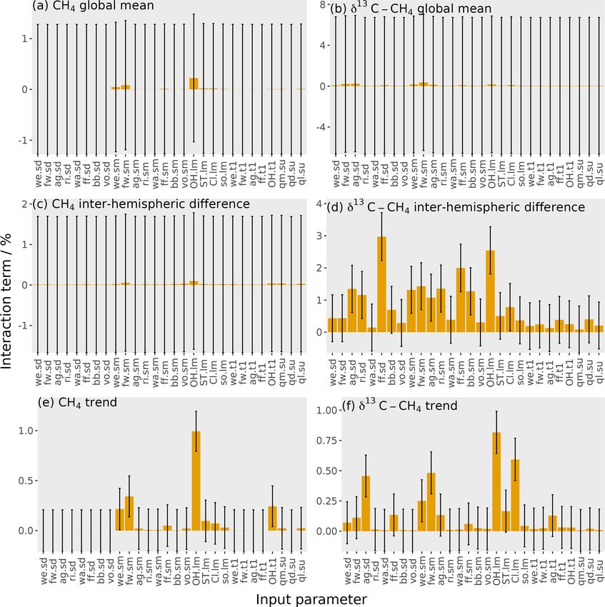
1718 A. C. Stell et al.: Methane budget sensitivity using Gaussian process emulation
Figure 1. The magnitude of the different sources and sinks contributing to the methane budget, derived from the ranges of bottom-up
estimates (Saunois et al., 2016). The blue bars are sources of methane, and the orange bars are sinks of methane. The error bars represent the
range of values used in this work, which are detailed in Sect. 2.2. The dashed black line shows the cut-off between the parameters that are
varied in this work and those that are not (see Sect. 2.2 for more detail).
Top-down (atmospheric-data-based) investigations of the sand (‰),
global methane budget have primarily relied on atmospheric 13
CH4
measurements of mole fractions made at “background” sites, 12 CH
4 sample
δ 13 C–CH4 = 13 − 1 × 1000, (1)
far from emission sources (e.g. Houweling et al., 1999; Chen CH4
and Prinn, 2006; Simpson et al., 2006; Rigby et al., 2008; 12 CH
4 standard
Bousquet et al., 2011; Rigby et al., 2017; Turner et al., 2017; where the standard is Pee Dee Belemnite (Coplen, 2011).
Naus et al., 2019), and/or remotely sensed observations (e.g. This global mean δ 13 C–CH4 has decreased since the renewed
Bergamaschi et al., 2013; Turner et al., 2016; Miller et al., methane growth in 2007 (Nisbet et al., 2016; Schaefer et al.,
2019). Measurements of the ratio of methane’s most abun- 2016).
dant isotopologues, 12 CH4 and 13 CH4 , have increasingly Many studies aiming to identify the cause of observed
been used to provide additional constraints on methane’s changes in atmospheric methane have relied on one-
sources and sinks (e.g. Bergamaschi et al., 1998; Quay et al., dimensional or two-dimensional (1D or 2D) box models of
1999; Nisbet et al., 2016; Rice et al., 2016; Schaefer et al., the atmosphere (e.g. Nisbet et al., 2016; Rigby et al., 2017;
2016; Rigby et al., 2017; Turner et al., 2017; Worden et al., Schaefer et al., 2016; Turner et al., 2017; Worden et al.,
2017; McNorton et al., 2018). The two isotopologues are 2017). A 2D box model typically splits the atmosphere into
emitted in different ratios from different sources (Whiticar a very small number of latitudinal and vertical boxes, within
and Schaefer, 2007; Schwietzke et al., 2016) and are fraction- which zonal mean mole fractions are calculated. These mod-
ated in the atmosphere by the isotopologues’ different rates els are known to be limited by their lack of interannual varia-
of loss with respect to the sinks (Saueressig et al., 2001). tion in transport and low spatial resolution. Naus et al. (2019)
These processes affect the ratio of 13 CH4 to 12 CH4 in the found that 2D box model parameters could be derived from
atmosphere, often described by δ 13 C–CH4 in parts per thou- a three-dimensional chemical transport model (3D CTM)
to combat these limitations, although some bias remained.
Atmos. Chem. Phys., 21, 1717–1736, 2021 https://doi.org/10.5194/acp-21-1717-2021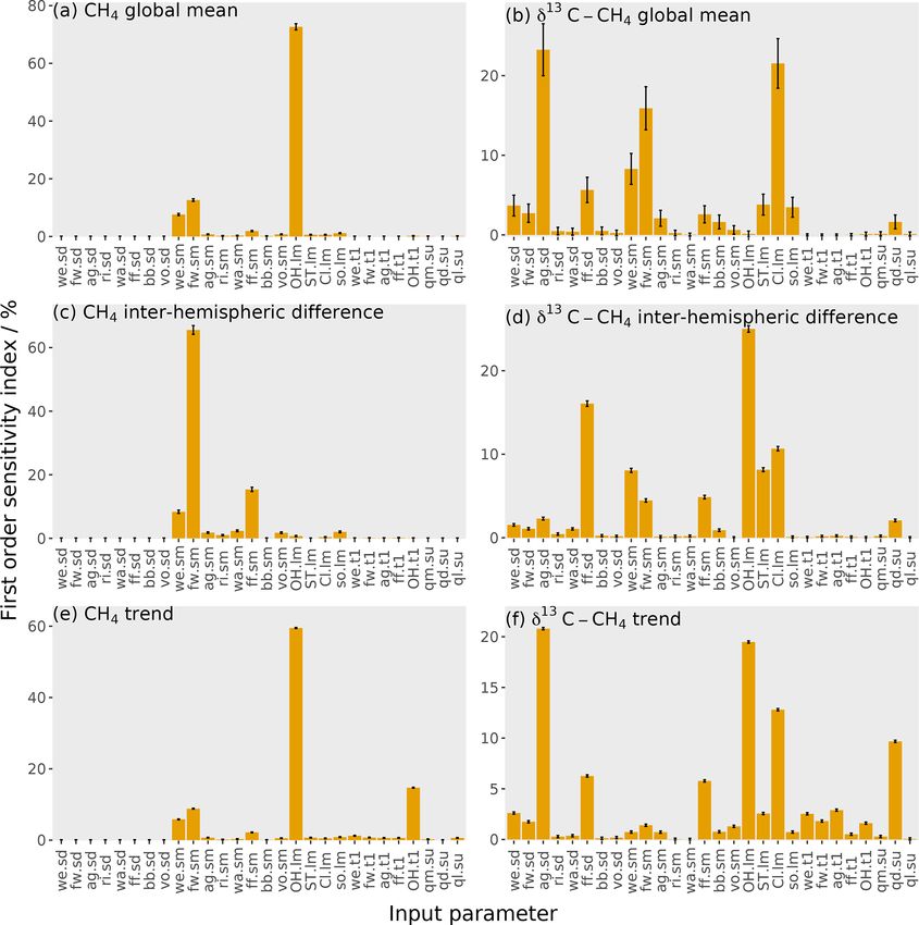
A. C. Stell et al.: Methane budget sensitivity using Gaussian process emulation                                             1719

Global inversions using 3D CTMs have been carried out (e.g.        2010). Such a sensitivity analysis, which as far as we are
Bousquet et al., 2011; Bergamaschi et al., 2013; Rice et al.,      aware has not yet been carried out for the sensitivity of at-
2016; McNorton et al., 2018). However, these studies often         mospheric methane to sources and sinks, will allow a better
rely on assumptions of linearity and Gaussian probability dis-     understanding of complex systems controlling atmospheric
tributions (which can be non-physical) and frequently omit         abundance of methane and future prioritisation of research
the exploration of some key parameters (e.g. by assuming           into its most important uncertain parameters.
fixed and known OH concentrations).
   The problem of efficiently estimating the relationship be-
tween uncertain inputs and observable outputs of a com-            2     Methods
plex model has been addressed in other fields using emu-
lation. An emulator is a statistical approximation to a more       This section begins with the motivation for using emulation
complex model, often using a Gaussian process (O’Hagan,            for sensitivity analysis (Sect. 2.1). Section 2.2 presents the
2006; Ebden, 2015). This technique has been applied to a           3D chemical transport model (CTM), for which the emula-
large variety of scientific problems, for example parameter        tor will act as a surrogate model, and its input parameters.
optimisation in models describing galaxy formation (Ver-           Section 2.3 outlines how the model was used to produce the
non et al., 2010), influenza epidemics (Farah et al., 2014),       data required to train the emulator. Then, Sect. 2.4 details
and the Greenland ice sheet (Chang et al., 2014); uncertainty      the mathematical background to Gaussian process emulators,
quantification in models of biospheric carbon flux (Kennedy        and their validation method is outlined in Sect. 2.5. Finally,
et al., 2008), aerosol effective radiative forcing (Regayre        Sect. 2.6 presents the sensitivity analysis method.
et al., 2018), and concentrations of cloud condensation nuclei
(Lee et al., 2012); and sensitivity analysis in aerosol models     2.1    Approach
(Lee et al., 2011) and chemistry–climate models (Wild et al.,
2020).                                                             In order to make running ∼ 106 simulations for a variance-
   In this work, we outline a set of emulators, which simu-        based sensitivity analysis feasible, emulators that are as com-
late atmospheric methane based on the inputs to a 3D CTM.          putationally cheap as 2D box models were built. The emula-
We limit our investigation to the simulation of hemispheric        tors built in this work are a statistical approximation to the
monthly average mole fraction and δ 13 C–CH4 , and therefore       3D CTM output of hemispheric median monthly methane
the emulators effectively serve as a more accurate 2D box          mole fraction and δ 13 C–CH4 . These emulators are much less
model. However, as discussed in Sect. 2.3, we anticipate that      computationally expensive than the 3D CTM, with a single
it would be trivial to extend the technique to the simulation of   evaluation taking 40 ms to run on a single core of a 1.6 GHz
model outputs at individual monitoring sites or for remotely       Intel Core i5 CPU in a laptop, compared to 4.5 h on 12 cores
sensed observations.                                               of a 2.4 GHz Intel E5-2680 v4 Broadwell CPU in a super-
   To demonstrate the value of the approach, we use the em-        computer for the 3D CTM. This computational expense re-
ulators to carry out a sensitivity analysis of atmospheric ob-     duction is possible while maintaining the spatial resolution
servations to the major uncertain components of the methane        in the emissions, loss fields, and transport as well as the in-
budget. One-at-a-time sensitivity tests (where only one input      terannual variability in transport lost in 2D box models. Ad-
parameter is perturbed at a time) are often used for complex       ditionally, this method assumes neither linear relationships
models due to the computational burden of the large number         between inputs and outputs nor non-interacting inputs, and
of simulations required to carry out a full sensitivity analy-     it allows a thorough exploration of the parameter space and
sis that allows for the possibility of interacting parameters.     error quantification that is difficult to achieve for 3D CTMs.
For example, this approach is effectively taken in previous        Perhaps the greatest drawback of the emulation method in
methane inverse-modelling studies, where sensitivities of ob-      this work is the small number of parameters that can be in-
servations to bulk regional flux changes are calculated us-        cluded, which is further discussed in Sect. 3.1.
ing finite differences (Fung et al., 1991; Hein et al., 1997;         In this work, a Gaussian process, which is a type of non-
Chen and Prinn, 2006; McNorton et al., 2018). A variance-          parametric curve fitting, emulates the 3D CTM (further ex-
based sensitivity analysis (Saltelli et al., 2000), where sensi-   plained in Sect. 2.4). There are other methods that could be
tivities are calculated using a large ensemble (typically mil-     used to create the emulators if the form of the function that
lions) of simulations, would be prohibitive with the compu-        maps model inputs to outputs is known, for example, linear
tational burden of a 3D CTM. However, here we show how             regression if the underlying function is linear. The Gaussian
a variance-based analysis can be performed using ∼ 102 3D          process achieves the same outcome but does not assume the
CTM simulations, requiring only modest computational re-           underlying functional form, and it requires only one main
sources. Using a fast emulator, we are able to thoroughly          assumption: the outputs follow a multivariate Gaussian dis-
sample the parameter space and also quantify parameter in-         tribution. Figure 2 shows a simple example of a 1D Gaus-
teractions, both of which can be critical for an accurate sen-     sian process emulator. The starting point for a Gaussian pro-
sitivity analysis of a complex model (Saltelli and Annoni,         cess is a set of known simulator outputs (the blue points in

https://doi.org/10.5194/acp-21-1717-2021                                             Atmos. Chem. Phys., 21, 1717–1736, 2021
1720                                           A. C. Stell et al.: Methane budget sensitivity using Gaussian process emulation

                                                                      2.2     The chemical transport model set-up and input
                                                                              parameter ranges

                                                                      2.2.1    The chemical transport model set-up

                                                                      This section describes how the 3D CTM, which the emula-
                                                                      tors will approximate, is set up. The model used is the well-
                                                                      established Model for Ozone and Related Chemical Trac-
                                                                      ers (MOZART) (Emmons et al., 2010), an offline global
                                                                      3D CTM. The MOZART model, run in a similar config-
                                                                      uration, has been used previously in global methane stud-
                                                                      ies and has been compared to other models and observa-
                                                                      tions (e.g. Patra et al., 2011). In this work, 56 vertical model
                                                                      levels were used, spanning from the Earth’s surface up to
                                                                      about 48 km. The model was run with a spatial resolution of
                                                                      12.00◦ N × 11.25◦ W and a time step of 1 h, with data output
                                                                      on a 6-hourly basis using MERRA reanalysis meteorological
                                                                      fields (Rienecker et al., 2011) from 1995 to 2012.
                                                                         The MOZART input parameters that are explored in this
                                                                      work describe the methane sources and losses in a similar
                                                                      way to Ganesan et al. (2018). The sources we use as inputs
                                                                      to MOZART are wetlands (Bloom et al., 2017), fresh water
Figure 2. A simple 1D example of a Gaussian process (GP). The         (see Supplement), agriculture (Crippa et al., 2018), rice (Yan
blue points represent known outputs of the simulator, and the black
                                                                      et al., 2009), waste (Crippa et al., 2018), fossil fuels (Crippa
line is the mean of the Gaussian process which interpolates between
the known outputs. The Gaussian-process-estimated uncertainty in
                                                                      et al., 2018), biomass burning (van der Werf et al., 2010),
its prediction is represented by the grey shading. The orange point   volcanoes (Etiope and Milkov, 2004), termites (Fung et al.,
is the Gaussian process prediction of an unknown simulator output     1991), hydrates (Fung et al., 1991), and oceans (Lambert and
and the orange bar represent the uncertainty in the prediction.       Schmidt, 1993; Houweling et al., 1999). The loss processes
                                                                      included in the model are the reactions of methane with the
                                                                      hydroxyl radical (OH) (offline, using fields generated by Spi-
Fig. 2), known as a training dataset. As long as a training           vakovsky et al., 2000), tropospheric chlorine radicals (Cl)
dataset exists or can be generated, this emulation method can         (Sherwen et al., 2016), net stratospheric loss (due to reaction
be applied to any simulator. The Gaussian process predicts            with Cl and O(1 D)) (Velders, 1995; Patra et al., 2011), and
the simulator output at untested inputs by interpolating be-          methanotrophic loss in soils (Murguia-Flores et al., 2018).
tween the training dataset. The prediction of the simulator           The model input fields are summarised in Table 1. The model
output (the black line in Fig. 2) is accompanied by an esti-          input fields are 2D for sources and the soil sink and 3D for
mated uncertainty in the prediction (the grey shading) that           the remaining sinks.
varies depending on how close the prediction input value is              The δ 13 C–CH4 observations are modelled by simulat-
to the values in the training dataset. A prediction of the sim-       ing both 12 CH4 and 13 CH4 . The emissions of these two
ulator output (the orange point in Fig. 2) has an uncertainty         species are determined by the literature source signatures
(shown by the orange bar), which is large if the input value          (Sect. 2.2.2), and the loss differs between the isotopologues
lies beyond the training dataset. Large errors like this are          according to the literature kinetic isotope effect (Sect. 2.2.2).
avoided in this work by using a training dataset range that              For each model simulation, MOZART was spun up us-
encompasses the full parameter uncertainty range explored             ing 30 years of repeating meteorology and sources and sinks
in our sensitivity analysis.                                          (nominally representative of the year 1995), starting from a
   The first step in this method is to decide on the range of         steady-state atmosphere. The model is then run for 1996–
possible input parameters to the simulator and run simula-            2012 with time-varying meteorology, emissions, and losses.
tions sampled over these ranges to form a training dataset.           To account for any transient signals during the first few years
A dataset of known model outputs that is independent of the           following spin-up (further discussed in Sect. 3.5), only 2000–
training dataset is used to validate the emulators. Once the          2012 was analysed. In each simulation, the fields in Table 1
emulators are validated, they can be used for the sensitivity         provide the spatial and temporal distribution of the emissions
analysis.                                                             and losses. The total global magnitude of the fields are scaled
                                                                      by the range of values discussed in Sect. 2.2.2 in order to in-
                                                                      vestigate the sensitivity of the methane observations.

Atmos. Chem. Phys., 21, 1717–1736, 2021                                                 https://doi.org/10.5194/acp-21-1717-2021
A. C. Stell et al.: Methane budget sensitivity using Gaussian process emulation 1721
Table 1. The emission and loss field input to MOZART, their literature sources, their temporal resolution, and the years covered by the fields.
Source Reference Temporal Years
resolution
Wetlands WetCHARTs (Bloom et al., 2017) Monthly 2001–2012 (1996–2000 are 2001 repeating)
Fresh water This work (see Supplement and Annual Climatology
available to download: Stell, 2020a)
Agriculture EDGAR 4.32 (Crippa et al., 2018) Annual 1996–2012
Rice Yan et al. (2009) Monthly 2000 repeating
Waste EDGAR 4.32 (Crippa et al., 2018) Annual 1996–2012
Fossil fuel (includes biofuel) EDGAR 4.32 (Crippa et al., 2018) Annual 1996–2012
Biomass burning GFED4s (van der Werf et al., 2010) Monthly 1997–2012 (1996 is the mean of all years)
Volcanoes Etiope and Milkov (2004) Annual Climatology
Termites Fung et al. (1991) Annual Climatology
Hydrates Fung et al. (1991) Annual Climatology
Oceans Lambert and Schmidt (1993); Annual Climatology
Houweling et al. (1999)
Loss
OH Spivakovsky et al. (2000) Monthly Climatology
Stratosphere Velders (1995); Patra et al. (2011) Monthly Climatology
Cl Sherwen et al. (2016) Monthly 2005 repeating
Soil Murguia-Flores et al. (2018) Monthly 1996–2009
(2010–2012 are 2009 repeating)
Rice is considered separately to agriculture and wetlands. Biofuel is included in fossil fuel rather than biomass burning. Agricultural burning is included in biomass
burning rather than agriculture. The mean of the WetCHARTs ensemble is used for wetland emissions.
2.2.2 The chemical transport model input ranges example, Wang et al. (2019) suggest a much smaller loss of
methane by reaction with Cl. The kinetic isotope effects were
We test the sensitivity to five properties of input source and held constant at typical literature values (King et al., 1989;
sink parameters: their source magnitudes, source δ 13 C–CH4 Tyler et al., 1994; Saueressig et al., 1995; Reeburgh et al.,
signatures, loss magnitudes, temporal trend variation for the 1997; Crowley et al., 1999; Snover and Quay, 2000; Tyler
largest emissions or losses, and initial conditions. Several mi- et al., 2000; Saueressig et al., 2001) derived as outlined in
nor terms in the methane budget (termites, hydrates, oceans, the Supplement. The reaction rates of methane with OH, Cl,
and loss kinetic isotope effects) were held constant, and so and O(1 D) were held constant at the values in Burkholder
are not included as inputs to the emulators, in order to sim- et al. (2015). While there is some uncertainty in these rate
plify the analysis. The uncertainty that results from these mi- constants, the sensitivity to this term will be similar to that of
nor terms being held constant is explored in Sect. 2.5. The their respective loss magnitudes. The ranges of loss parame-
range of possible values for the chosen parameters must be ter values used in this work are given in Table 2.
identified so that a set of MOZART simulations over these The default temporal trends of the emissions and losses
ranges can be created, which forms the training dataset for from 1996 to 2012 are set by the input fields in Table 1.
the emulators. The overall inventory or process model trend for the five
The ranges of possible source magnitudes were based on largest methane emissions or losses (OH, wetlands, fresh wa-
the ranges of compiled literature values in Saunois et al. ter, agriculture, and fossil fuels) was allowed to vary by a
(2016). The minimum and maximum values from Saunois linear trend of ± 20 % (± 1.2 % yr−1 ). For example, a trend
et al. (2016) have been decreased and increased, respectively, parameter that reduces a term by 20 % is applied as a 10 %
by 10 % in this work as Saunois et al. (2016) do not include increase in the first year, decreasing to no change in the mid-
the uncertainties in the compiled studies or outliers in their dle of the time series, and then decreasing to −10 % in the
ranges. The ranges of possible δ 13 C–CH4 source signatures final year.
were the 3-standard-deviation ranges in Schwietzke et al. Three parameters were varied during the spin-up: the total
(2016). The ranges of source parameter values used in this source magnitude, the total source δ 13 C–CH4 signature, and
work are given in Table 2. an overall imbalance between the source and sink. Table 2
The ranges of possible loss magnitudes were based on gives the range of these spin-up parameters. The range of
Saunois et al. (2016) in the same way as the sources. These the spin-up total source magnitude was derived by consider-
ranges do not include some more recent literature values; for ing the minimum and maximum of the sum of the sources in
https://doi.org/10.5194/acp-21-1717-2021 Atmos. Chem. Phys., 21, 1717–1736, 20211722 A. C. Stell et al.: Methane budget sensitivity using Gaussian process emulation
Table 2. The range of the total source δ 13 C–CH4 signature exhibited substantial above-baseline variability in the model
is constrained to values where the resulting January 1996 (likely an artefact of the coarse model resolution).
initial-condition field has a global surface δ 13 C–CH4 ap- The MOZART outputs are monthly time series describ-
proximately matching observations (−47.3 ± 0.6 ‰). Simi- ing the Southern Hemisphere mole fraction, the Northern
larly, the range of the imbalance between the source and sink Hemisphere mole fraction, the Southern Hemisphere δ 13 C–
is constrained to values where the resulting January 1996 CH4 , and the Northern Hemisphere δ 13 C–CH4 . These four
initial-condition field has a global surface methane mole frac- 3D CTM outputs are the quantities that the Gaussian pro-
tion approximately matching observations (1760 ± 30 ppb). cesses emulate. However, it should be trivial to extend this
However, the January 1996 initial condition can go beyond to individual grid cells of the 3D CTM in future work. This
these observed ranges by varying the other two spin-up pa- number of emulators is feasible as the same training dataset
rameters. The range of initial-condition values is larger than could be used, and the computational burden of both building
that considered in previous methane-modelling studies, and it and running the emulator is far smaller than creating the 3D
therefore may be an overestimate. However, given that con- CTM training simulations.
straints are only typically provided based on surface obser- In order to explore sensitivities to quantities that are more
vations, whereas the initial model fields are 3D, extending often used (either implicitly or explicitly) to inform the
from the surface to the upper stratosphere, it is very difficult global methane budget, the hemispheric outputs are com-
to determine how uncertain the initial conditions truly are. bined as a global mean, inter-hemispheric difference, and
trend of the mole fraction and δ 13 C–CH4 . The global mean is
defined as the temporal mean of the mean over the northern
2.3 Creating the chemical transport model training
and southern hemispheres for all months between 2000 and
and validation datasets
2012. The inter-hemispheric difference is the temporal mean
over the Northern Hemisphere minus the Southern Hemi-
This section discusses the generation of the training and vali- sphere, averaged over all months between 2000 and 2012.
dation datasets, which is the most computationally expensive The trend is defined as the global mean in December 2012
part of the analysis as repeated runs of the 3D CTM are re- minus December 2000.
quired. The training and validation datasets were designed to
give accurate emulators for the whole range of the parame- 2.4 Gaussian process emulators
ter values in Table 2. Therefore, the sets of input parameters
in the datasets should be evenly spaced so that every possi- 2.4.1 The basics of Gaussian process emulation
ble input parameter set is close to training data. Hence, each
parameter described in Table 2 is assigned a uniform prob- The Gaussian process is defined by two functions that vary
ability distribution over the range given. In order to sample depending on the input parameter values: the mean function
from the distributions in a way that effectively covers the in- and the covariance function. It is sufficient to have a mean
put parameter space, a maximin Latin hypercube was used function of 0, though in this work, a multiple linear regres-
(McKay et al., 1979; Morris and Mitchell, 1995). A training sion was chosen as the system is close to linear. A linear
dataset of 270 MOZART simulations was created and used mean function does not stop the Gaussian process from being
to build the Gaussian process emulators. We chose 270 sim- able to model non-linear relationships. The covariance func-
ulations as it was found to provide a balance between the tion is a measure of the similarity of input sets, and as the
accuracy of the emulator and the computational expense of distance between the inputs increase, the value of the func-
generating training simulations. This is further discussed in tion decreases. In this work we use the squared exponential
the Supplement. An independent maximin Latin hypercube covariance function as there are no discontinuities or sharp
design of 90 MOZART simulations was created as a valida- changes in the methane observations due to input parameter
tion dataset, which was used to evaluate the emulators. variation. The (i, j )th element of the covariance matrix (K)
Although observations were not required for this study, is given by
for consistency with observed trends, we opted to calculate m
!
hemispheric averages based on mole fractions and δ 13 C– 2
X (xk,i − xk,j )2
ηij = σf exp − , (2)
CH4 at grid cells where baseline observations were made k=1 lk2
by the Global Monitoring Laboratory (GML) Carbon Cy-
cle group, part of the US National Oceanic and Atmospheric where the maximum covariance is σf2 , xk is the value of the
Administration (NOAA) (Dlugokencky et al., 1994, 2017), kth input parameter, and lk is the length-scale parameter to
and the Institute of Arctic and Alpine Research (INSTAAR) be optimised during training.
(Miller et al., 2002; White et al., 2018), respectively. Mea- In this work, the input parameters are the 28 scaling factors
surement stations that do not have approximately continuous in Table 2, and the outputs are the MOZART hemispheric av-
records for the period of interest (more than 9 out of 13 years) erage mole fraction and δ 13 C–CH4 values. The prediction of
were discarded. We also discarded measurement sites that an output value (y ∗ ) at a set of input parameters (x ∗ ) sam-
Atmos. Chem. Phys., 21, 1717–1736, 2021 https://doi.org/10.5194/acp-21-1717-2021A. C. Stell et al.: Methane budget sensitivity using Gaussian process emulation 1723
Table 2. A table of the ranges of the 28 input parameters to MOZART that were varied in the training simulations, hence also in the emulators,
and in the sensitivity analysis. Where one value is given, the value is held constant for all training simulations. Where two values are given,
they are the lower and upper limit, respectively.
Source Magnitude Delta value 1996–2012 trend
(Tg yr−1 ) (‰) (% yr−1 )
Wetlands 136, 250 −63.3, −59.7 −1.2, 1.2
Fresh water 54, 198 −64.6, −59.8 −1.2, 1.2
Agriculture 86, 122 −75.2, −58.4 −1.2, 1.2
Rice 21, 40 −66.0, −58.2
Waste 46, 69 −57.7, −53.5
Fossil fuel (includes biofuel) 104, 162 −45.1, −38.4 −1.2, 1.2
Biomass burning 14, 29 −27.9, −16.5
Volcanoes 27, 62 −46.1, −41.9
Termites 9.6 −65.0
Hydrates 0 −62.2
Oceans 16 −57.9
Loss Magnitude Kinetic isotope 1996–2012 Trend
(Tg yr−1 ) effect (% yr−1 )
OH 414, 730 1.0039 −1.2, 1.2
Stratosphere 6, 55 1.0397
Cl 12, 41 1.0640
Soil 8, 52 1.0215
Spin-up Magnitude Delta value
(Tg yr−1 ) (‰)
Spin-up source 495, 976 −55.6, −53.7
Spin-up source minus loss 23.2, 62.8
The trend magnitudes are based on a percentage of the original field read into the model, so they could equally
be expressed as ± 2.0 Tg yr−1 for wetlands, ± 1.5 Tg yr−1 for fresh water, ± 1.3 Tg yr−1 for agriculture,
± 1.3 Tg yr−1 for fossil fuels, and ± 6.2 Tg yr−1 for OH.
ples from the joint multivariate Gaussian distribution of the 2.4.2 Gaussian process emulation for time series
training data (y) and the predicted values, which follows outputs
K(x, x) K(x, x ∗ )
y ∗ Each MOZART output is a time series of 156 months (12
∼ N m(x ), , (3)
y∗ K(x ∗ , x) K(x ∗ , x ∗ ) months for each of 13 years) of hemispheric median mole
fraction or δ 13 C–CH4 . These 156 monthly outputs are highly
where m is the mean function, and x is the training dataset correlated in time, which can be exploited in the design of
inputs. This means that the expected value of y ∗ is the emulator covariance matrix to minimise information loss.
There will also be correlations in space between the northern-
E(y ∗ ) = m(x ∗ ) + K(x ∗ , x)K(x, x)−1 y, (4)
and southern-hemispheric outputs, but these correlations are
and the uncertainty, in terms of variance, in the estimate is not considered in this work. The chosen covariance matrix
(6) is composed of the Kronecker product of a temporal
V (y ∗ ) = K(x ∗ , x ∗ ) − K(x ∗ , x)K(x, x)−1 K(x, x ∗ ). (5) covariance matrix (6 t ) and a parameter covariance matrix
(6 x ),
The Gaussian process emulation method is further described
6 = 6t ⊗ 6x . (6)
in Rasmussen and Williams (2006), and some simple tutori-
als are available in O’Hagan (2006) and Ebden (2015). The elements of 6 t and 6 x are described by ζij and ηij ,
respectively. The chosen temporal covariance is a first-order
autoregressive model (its value depends only on the previous
month), and its (i, j )th element is
ρ |ti −tj |
ζij = , (7)
1 − ρ2
https://doi.org/10.5194/acp-21-1717-2021 Atmos. Chem. Phys., 21, 1717–1736, 20211724 A. C. Stell et al.: Methane budget sensitivity using Gaussian process emulation
where ρ is the autocorrelation parameter, and t is the month. In a variance-based sensitivity analysis, the model sensi-
The chosen parameter covariance is a squared exponential, tivity is quantified using sensitivity indices. These indices
and its (i, j )th element is given by Eq. (2). measure the proportion of the output variance caused by an
The emulator parameters (ρ in Eq. 7, σf and lk in Eq. 2) input parameter being varied over its possible range (Saltelli
are optimised by maximising the log-likelihood function et al., 2000). In this work, two sensitivity indices are calcu-
lated: the first-order and total effect indices. The first-order
1 1 sensitivity index reflects the proportion of the variance in the
log(L) ∝ − (y − m(x))T 6 −1 (y − m(x)) − log(|6|). (8)
2 2 output that can be attributed to a single parameter. This can
be calculated as
This log-likelihood function is maximised using a bounds-
constrained quasi-Newton method (Gay, 1990) started from V [E(y|xk )]
28 different random points, and the emulator with the maxi- Sk = , (9)
V (y)
mum log-likelihood is chosen. This set-up uses an adaptation
of the R package Stilt (Olson et al., 2018). where V [E(y|xk )] is the variance in the expected value of
the emulator output y given the value of parameter xk , and
2.5 Validation of the emulators V (y) is the variance in the emulator output caused by all pa-
rameters.
It is important to check that the emulators are an accurate The total effect index is the proportion of the output vari-
approximation of the 3D CTM before they are used. The val- ance that can be explained by a single parameter and its in-
idation dataset is used to confirm this because it contains teractions with other parameters. This can be calculated as
inputs and known 3D CTM outputs that the emulator was
not trained on. The emulator predictions for the validation V [E(y|x∼k )]
ST k = 1 − , (10)
dataset inputs can be compared to the 3D CTM output, and V (y)
these differences reveal how accurate the approximation is.
There are several graphical comparison methods presented where V [E(y|x∼k )] is the variance in y caused by all pa-
in the Supplement, but the main focus is the absolute error rameters except xk . A parameter’s interactions with all other
in emulation. For the emulators to be useful, their error in parameters can be calculated by subtracting the first-order
emulating the CTM output must be much smaller than a rea- sensitivity index from the total sensitivity index. These sen-
sonable estimate of the other errors in the system. sitivity indices were calculated using Monte Carlo methods
The error in a complex model is difficult to calculate, and (Saltelli et al., 2000), and further details are given in the Sup-
so it is often ignored; expert judgement is used; or estimates plement.
of model–data mismatch uncertainties are approximated, e.g.
based on spatial or temporal variability in the model output 3 Results and discussion
in the vicinity of observation points (e.g. Chen and Prinn,
2006). In this work, the uncertainty in the 3D CTM is ap- Here, we demonstrate the accuracy of the emulators and
proximated by the uncertainty due to the invariant param- show how they can be applied to a sensitivity study of the
eters (as in Vernon et al., 2010). The invariant parameters global methane budget. Section 3.1 compares the 3D chem-
and their investigated ranges are given in Table 3. The uncer- ical transport model (CTM) training dataset to the observa-
tainty was calculated with a maximin Latin hypercube design tions in order to check that the observations lie within the
of 90 MOZART simulations, where variations were allowed envelope of the model output ensemble. Section 3.2 exam-
only in those parameters held constant in the emulator train- ines the size of the 3D CTM invariant parameter error, which
ing dataset. This invariant parameter error does not include is compared to the emulator error in Sect. 3.3 in order to
many other sources of error (e.g. model transport uncertain- justify the use of emulation. The Gaussian process emula-
ties are not addressed) and higher-order “invariant parameter tion method is then shown to be warranted by comparison
errors” (e.g. erroneous trends or spatial distributions), so it to a simpler multiple linear regression in Sect. 3.4. Having
can be considered a lower bound of the total 3D CTM error. demonstrated the utility of the method, a sensitivity analysis
is presented in Sect. 3.5.
2.6 Calculation of sensitivity indices
3.1 Comparison of 3D chemical transport model
The sensitivity analysis, using the validated emulators, iden- training dataset to observations
tifies how sensitive the 3D CTM outputs are to changes in the
inputs. A variance-based sensitivity analysis requires ∼ 106 The training dataset is compared to observations to check
simulations, which would be unfeasible using the 3D CTM that the observations lie within the envelope of the MOZART
as the model is so computationally expensive. By using an output ensemble. The MOZART simulations used to train
emulator, the only 3D CTM simulations required are those the emulators are shown in Fig. 3. The outputs that are con-
needed to train the emulators. sidered in the sensitivity analysis (the temporal mean of the
Atmos. Chem. Phys., 21, 1717–1736, 2021 https://doi.org/10.5194/acp-21-1717-2021A. C. Stell et al.: Methane budget sensitivity using Gaussian process emulation 1725
Table 3. The ranges of the invariant parameters explored (from the literature as in Sect. 2.2.2), where the first number is the minimum, and
the second number is the maximum. The 13 CH4 A factor is the Arrhenius pre-exponential factor, which is changed in the model to describe
uncertainty in the kinetic isotope effect with respect to the losses. The OH and 13 CH4 A factor was also considered, but MOZART only
allows the rate constant to be input with two decimal places, and the OH and 13 CH4 A factor is constant when given to two decimal places
over the range of kinetic isotope effects explored.
Term Magnitude (Tg yr−1 ) Delta value (‰) 13 CH A factor
4
Termites 5.0, 14.2 −66.7, −63.3
Hydrates 0.0, 0.9 −63.0, −61.4
Oceans 8.3, 23.7 −51.7, −44.1
Soil −24.0, −19.0
Tropospheric chlorine 6.66, 6.68 × 10⁻¹² cm3 molec.−1 s−1
Stratosphere 0.958, 0.966 s−1
Methane loss by soil was input to the model as negative emissions; hence its isotopic fractionation is not characterised by an A factor.
global mean, the temporal mean of the inter-hemispheric dif- Over the 13-year period of our study, the mean invariant pa-
ference, and the trend in the global mean (Sect. 2.3) for the rameter uncertainty is about 10 ppb and 0.1 ‰ for the mole
mole fraction and δ 13 C–CH4 ) are presented in Fig. 4. In these fraction and δ 13 C–CH4 , respectively. These values are gen-
figures, the distribution of the MOZART simulations (in or- erally slightly larger than the estimate of the combined mea-
ange) is compared to the NOAA and INSTAAR atmospheric surement and model representation uncertainty, which exam-
observations presented in Rigby et al. (2017) (in black) (de- ines the limited temporal and spatial resolution of the model
rived from a slightly different subset of measurement stations (further details in the Supplement). Additionally, the invari-
to those used in this work). ant parameter uncertainty is large compared to atmospheric-
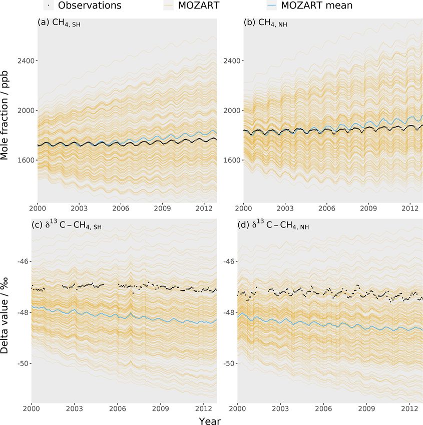
These figures demonstrate the large range of methane methane trends (e.g. between 2000 and 2012, the methane
mole fraction and δ 13 C–CH4 values covered by the training mole fraction and δ 13 C–CH4 changed by around 40 ppb and
dataset. This is caused by the large range of emission, loss, −0.1 ‰, respectively). Furthermore, these uncertainties are
and initial-condition values (Sect. 2.2.2). Additionally, the highly correlated through the study period and therefore ef-
figures show that the observations are within the MOZART fectively act as a substantial bias. The omission of this sub-
range for all outputs. stantial source of error will likely be leading to an underes-
These figures also show that the range of MOZART inter- timation of uncertainties in emissions and losses derived in
hemispheric-difference values is small compared to the range inverse-modelling studies or may contribute to the misallo-
of global mean and trend values. Ideally, the spatial distri- cation of some emission or loss to particular processes.
butions of the emissions and losses would also be param-
eterised, allowing greater variation in the inter-hemispheric 3.3 Validation of the emulators
differences. However, only a limited number of parameters
can be included in the Gaussian process emulation method Before using the emulators, it is important to check that
of this work. The more parameters, the more 3D CTM simu- they reproduce the 3D CTM output well. A more complete
lations are required to train the emulator and the slower com- analysis can be found in the Supplement, which shows that
putation becomes. Therefore, only up to about 30 parameters the emulator is an unbiased representation of the 3D CTM.
are typically included in a Gaussian process, whereas meth- The emulator error was calculated by predicting the valida-
ods such as adjoint models (e.g. Bousquet et al., 2011; Berga- tion dataset (Sect. 2.3) and comparing the predictions to the
maschi et al., 2013) can include thousands of parameters. MOZART output using the root-mean-square error (RMSE),
v
u n
3.2 The 3D chemical transport model invariant uX (y em,i − y mzt,i )2
RMSE = t , (11)
parameter error i=1
n
The MOZART invariant parameter error (Sect. 2.5), as far as where y em is the emulator output, y mzt is the MOZART out-
we are aware, has not been considered in previous methane- put, and n is the number of simulations being compared. The
modelling studies. This error was calculated as the standard RMSE was calculated to be about 1.0 ppb and 0.05 ‰ for
deviation in the output of the set of simulations where pa- the mole fraction and δ 13 C–CH4 , respectively. This emula-
rameters not included in the emulator training dataset (fluxes tor error is small when compared to the MOZART invariant
from termites, hydrates, and oceans as well as isotopic frac- parameter error (Sect. 2.5) in Fig. 5.
tionation by soil, tropospheric Cl, and stratospheric losses) As the MOZART invariant parameter error is significantly
were perturbed within their uncertainty ranges (Table 3). larger than the emulator error, it is possible to use a less ac-
https://doi.org/10.5194/acp-21-1717-2021 Atmos. Chem. Phys., 21, 1717–1736, 20211726 A. C. Stell et al.: Methane budget sensitivity using Gaussian process emulation
Figure 3. The MOZART training dataset (orange lines), the mean MOZART output (blue line), and the observations (black line) for each
of the four emulators: (a) the Southern Hemisphere mole fraction, (b) the Northern Hemisphere mole fraction, (c) the Southern Hemisphere
δ 13 C–CH4 , and (d) the Northern Hemisphere δ 13 C–CH4 . The observations are hemispheric averages based on NOAA and INSTAAR data
(derived from a slightly different subset of measurement stations to those used in this work) presented in Rigby et al. (2017).
curate emulator that requires fewer training simulations. As Therefore, this section compares the performance of multi-
making the training dataset is the longest step in the process, ple linear regression and the Gaussian process as emulators
this would be beneficial for more time-consuming higher- of the 3D CTM.
resolution models. In the case of MOZART, we find that only The residuals for the global mean between the 3D CTM
around 90 simulations may be required, which is further dis- validation dataset and the predictions from the two meth-
cussed in the Supplement. ods (multiple linear regression and the Gaussian process) are
compared in Fig. 6. The Gaussian process residuals, with an
3.4 Comparison of multiple linear regression and the RMSE of 0.9 ppb and 0.05 ‰, are much smaller than for mul-
Gaussian process tiple linear regression, for which they are 19 ppb and 0.14 ‰.
In comparison to the MOZART invariant parameter error
Previous studies (e.g. McNorton et al., 2018) have assumed (10 ppb and 0.1 ‰), the multiple linear regression residuals
that for small changes in the source and loss magnitudes, the are large, unlike the Gaussian process (Sect. 3.3). Therefore,
relationship between methane sources and losses and atmo- the multiple linear regression struggles to emulate MOZART
spheric mole fraction and δ 13 C–CH4 is linear and that the with the required accuracy.
parameters do not interact (Sect. 3.5). If these two condi- The multiple linear regression accuracy can be improved
tions are true or close to true, then multiple linear regres- by considering the non-linearity of the mole fraction with re-
sion would be able to emulate the 3D CTM. Multiple linear spect to the OH loss. By using a log-transformed OH param-
regression might be preferred to a Gaussian process as it re- eter to estimate the mole fraction, the RMSE becomes 11 ppb
quires a smaller training dataset (hence fewer 3D CTM sim- (the complete residual distribution is shown in Fig. 6). Mul-
ulations) and is conceptually and computationally simpler.
Atmos. Chem. Phys., 21, 1717–1736, 2021 https://doi.org/10.5194/acp-21-1717-2021A. C. Stell et al.: Methane budget sensitivity using Gaussian process emulation 1727
Figure 4. Histograms of the 270 3D CTM training simulations for six outputs: (a) mole fraction global mean, (b) δ 13 C–CH4 global mean,
(c) mole fraction inter-hemispheric difference, (d) δ 13 C–CH4 inter-hemispheric difference, (e) mole fraction trend, and (f) δ 13 C–CH4 trend.
The black line is the corresponding value for the NOAA and INSTAAR atmospheric observations (Sect. 2.3), which are hemispheric averages
(derived from a slightly different subset of measurement stations to those used in this work) presented in Rigby et al. (2017).
tiple linear regression using a log-transformed OH parameter The sensitivity of the global mean mole fraction is shown
still has a significantly larger RMSE than the Gaussian pro- in Fig. 7a and is dominated by the OH loss magnitude (73 %),
cess, implying that the remaining small non-linearities and with considerable contributions from the freshwater (13 %)
parameter interactions are important for predicting the out- and wetlands (8 %) source magnitudes. These sensitivities
put value. This finding suggests that inverse-modelling stud- follow the absolute size of the uncertainty in the source and
ies that have assumed linear and independent sensitivities be- loss magnitudes seen in Fig. 1 and are therefore relatively un-
tween observations and source and sink parameters may have surprising. However, these results highlight the overwhelm-
underestimated their posterior uncertainties. ing importance of global mean OH concentration in deter-
mining the global methane mole fraction and the major influ-
3.5 Using the emulators for sensitivity analysis ence of freshwater emission uncertainties, which have largely
been ignored in recent global modelling studies.
Figure 7b shows the sensitivity of the global mean δ 13 C–
3.5.1 First-order sensitivity indices CH4 to each input parameter. The parameters that this out-
put is most sensitive to are the agricultural source δ 13 C–
In this section, we examine the sensitivity of the MOZART CH4 signature (23 %), the Cl sink magnitude (22 %), and the
outputs to the input parameters describing methane sources freshwater source magnitude (16 %), with a couple of other
and sinks. This sensitivity is explored using the first-order parameters contributing substantially: the wetlands source
sensitivity indices (Eq. 9) in Fig. 7, which show the propor- magnitude (8 %) and the fossil fuels δ 13 C–CH4 signature
tion of the variance of the MOZART output caused by vary- (6 %). As the mole fraction and δ 13 C–CH4 are most sensi-
ing each parameter.
https://doi.org/10.5194/acp-21-1717-2021 Atmos. Chem. Phys., 21, 1717–1736, 20211728 A. C. Stell et al.: Methane budget sensitivity using Gaussian process emulation Figure 5. The MOZART error (blue line), emulator error (green line), and total error (MOZART and emulator errors added in quadrature) (black line) for each of the four emulators: (a) the Southern Hemisphere mole fraction, (b) the Northern Hemisphere mole fraction, (c) the Southern Hemisphere δ 13 C–CH4 , and (d) the Northern Hemisphere δ 13 C–CH4 . tive to different parameters, this means that the δ 13 C–CH4 ing, so it has a large impact on the δ 13 C–CH4 . The third- could be a useful additional measurement for constraining highest contribution is from the freshwater source magnitude the methane budget. However, two of the parameters that as this source has a large uncertainty, and its source δ 13 C– δ 13 C–CH4 is most sensitive to are δ 13 C–CH4 -specific (the CH4 signature is substantially more negative than the atmo- agricultural and fossil fuel source δ 13 C–CH4 signatures) and spheric δ 13 C–CH4 . Interestingly, in this investigation, global so do not, on their own, add information about the mag- mean δ 13 C–CH4 has almost no sensitivity to the magnitude nitudes of the different methane sources and sinks. Unlike of the OH sink. As we show in the Supplement, this finding the global mean mole fraction, the ordering of the param- is because the transient response of global mean δ 13 C–CH4 eters to which δ 13 C–CH4 is most sensitive does not sim- to a change in the OH concentration exhibits a sign change, ply follow the absolute magnitude of uncertainty in the in- which coincidentally falls almost exactly at the centre of the put parameters. The global mean δ 13 C–CH4 is most sensitive period we investigate. Therefore, while the change in OH to the agricultural source δ 13 C–CH4 signature, which has a concentration at the beginning of our simulation causes a sig- large uncertainty compared to other source δ 13 C–CH4 signa- nificant change in global δ 13 C–CH4 during the years 2000 tures. Additionally, this source δ 13 C–CH4 signature is sub- and 2012 (with opposite signs), these changes roughly can- stantially more negative than the atmospheric δ 13 C–CH4 in cel in the 2000–2012 mean. comparison to other sources, and so this parameter results in The mole fraction inter-hemispheric difference (the tem- a large output variance in the global mean δ 13 C–CH4 . The poral mean over the Northern Hemisphere minus the South- second-highest contribution to the output variance is the Cl ern Hemisphere as in Sect. 2.3) is most sensitive to the fresh- loss magnitude, which has a small uncertainty in comparison water (66 %), fossil fuel (15 %), and wetlands (8 %) source to other parameters. However, this loss is highly fractionat- magnitudes, as shown in Fig. 7c. The sensitivity to these pa- Atmos. Chem. Phys., 21, 1717–1736, 2021 https://doi.org/10.5194/acp-21-1717-2021
A. C. Stell et al.: Methane budget sensitivity using Gaussian process emulation                                                       1729

Figure 6. The residuals for the global mean between the different emulation methods (in different colours) and the true MOZART output
for (a) methane mole fraction and (b) δ 13 C–CH4 . Each emulator is built using a Gaussian process (GP) (grey) or multiple linear regression
(MLR) (orange). The mole fraction has an additional emulator: a multiple linear regression with log-transformed OH (blue).

rameters is due to their large uncertainties and large differ-          somewhat coincidental, as discussed above and in the Sup-
ences in emissions between the two hemispheres. The OH                  plement).
loss magnitude, which has the largest uncertainty in any pa-               The sensitivity of the mole fraction trend (the global mean
rameter, has been assumed to be close to equally distributed            in December 2012 minus December 2000 as in Sect. 2.3) is
between the hemispheres (Patra et al., 2014), hence its low             shown in Fig. 7e. The sensitivity is dominated by a single pa-
sensitivity with respect to this output. However, had the un-           rameter: 59 % of the variance is caused by the uncertainty in
certainty in the hemispheric distribution of OH been included           the OH loss magnitude. The OH loss trend (15 %), freshwa-
in our analysis, it would likely have explained a larger pro-           ter source magnitude (9 %), and wetlands source magnitude
portion of this sensitivity. The dominant role of freshwater            (6 %) also contribute significantly. The OH loss parameter’s
emission uncertainty in determining the inter-hemispheric               importance for the output mole fraction value stems from the
difference further highlights the need to better understand             large uncertainty in the OH loss.
this part of the methane budget.                                           The δ 13 C–CH4 trend sensitivity is shown in Fig. 7f. The
   Figure 7d shows the sensitivity of the δ 13 C–CH4 inter-             trend is most sensitive to the agricultural source δ 13 C–CH4
hemispheric difference. The parameters that the δ 13 C–CH4              signature (21 %), the OH loss magnitude (19 %), the Cl loss
inter-hemispheric difference is most sensitive to are the OH            magnitude (13 %), and the spin-up source δ 13 C–CH4 signa-
loss magnitude (25 %), the fossil fuel source δ 13 C–CH4 sig-           ture (10 %). There are additional contributions from the fos-
nature (16 %), and the Cl sink magnitude (11 %). There are              sil fuel source δ 13 C–CH4 signature (6 %) and the fossil fuel
also significant contributions from the wetlands source mag-            source magnitude (6 %). Parameters that can change the at-
nitude (8 %) and the stratospheric loss magnitude (8 %). The            mospheric global mean δ 13 C–CH4 will also affect the trend
parameters to which the δ 13 C–CH4 inter-hemispheric differ-            (e.g. the agricultural source δ 13 C–CH4 and the Cl loss mag-
ence is most sensitive are similar to those that most strongly          nitude). Additionally, the trend is sensitive to the OH loss
influence the global mean δ 13 C–CH4 but with a higher sen-             magnitude, despite the global mean being insensitive to this
sitivity to parameters with a large inter-hemispheric differ-           parameter. This sensitivity to OH is explained by the slow
ence (e.g. fossil fuels). The exception is the sensitivity to           (and somewhat counter-intuitive) way that changes in the
the OH loss magnitude, which strongly impacts the inter-                δ 13 C–CH4 propagate through the atmosphere and will be de-
hemispheric difference but not the global mean (which is                pendent on the time period investigated, which is explained
                                                                        in detail in the Supplement. The δ 13 C–CH4 trend is also sen-

https://doi.org/10.5194/acp-21-1717-2021                                                   Atmos. Chem. Phys., 21, 1717–1736, 2021
1730 A. C. Stell et al.: Methane budget sensitivity using Gaussian process emulation Figure 7. The orange bars show the first-order sensitivity coefficients to the input parameters, with the error bars showing the uncertainty in these indices (calculated using bootstrap resampling; see Supplement). Each panel is for one of six outputs: (a) mole fraction global mean, (b) δ 13 C–CH4 global mean, (c) mole fraction inter-hemispheric difference, (d) δ 13 C–CH4 inter-hemispheric difference, (e) mole fraction trend, and (f) δ 13 C–CH4 trend. The values given here are for the temporal mean of the time series. The input parameter codes are given by a combination of a two-character code giving the source or loss (wetlands, we; fresh water, fw; agriculture, ag; rice, ri; waste, wa; fossil fuels, ff; biomass burning, bb; volcanoes, vo; hydroxyl radical, OH; stratospheric, ST; Cl radical, Cl; soil, so; total source magnitude, qm; total source δ 13 C–CH4 signature, qd; total loss imbalance, ql) and another code giving the type of parameter (source δ 13 C–CH4 signature, sd; source magnitude, sm; loss magnitude, lm; temporal trend, t1; spin-up, su). sitive to the spin-up because of the slow response time in the a serious challenge if δ 13 C–CH4 observations are to be used atmospheric δ 13 C–CH4 , meaning that the trend is strongly to estimate the recent changes in the methane budget. dependent on its initial value (Tans, 1997). A wide range These first-order sensitivity indices demonstrate several of spin-up source δ 13 C–CH4 signature values (Table 2) are key challenges in methane inverse-modelling studies. Three examined in this work; however the importance of the spin- parameters that the mole fraction and δ 13 C–CH4 are highly up applies to even small ranges. For example, if the spin- sensitive to are often not explored in methane modelling: the up source δ 13 C–CH4 signature is perturbed by 0.1 ‰ from OH loss is often assumed to be known (e.g. Schaefer et al., the initial median parameter values, the output atmospheric- 2016; Worden et al., 2017), as is the Cl loss (e.g. Nisbet δ 13 C–CH4 trend changes by 0.04 ‰, almost half the ob- et al., 2016; Rigby et al., 2017), or the Cl loss is omitted served δ 13 C–CH4 trend during this period. Therefore, con- (e.g. Turner et al., 2017). Furthermore, freshwater emissions straining the initial conditions throughout the atmosphere is have not been included as an independent source in global Atmos. Chem. Phys., 21, 1717–1736, 2021 https://doi.org/10.5194/acp-21-1717-2021
You can also read