Geometric controls of tidewater glacier dynamics - The Cryosphere
←
→
Page content transcription
If your browser does not render page correctly, please read the page content below
The Cryosphere, 16, 581–601, 2022
https://doi.org/10.5194/tc-16-581-2022
© Author(s) 2022. This work is distributed under
the Creative Commons Attribution 4.0 License.

Geometric controls of tidewater glacier dynamics
Thomas Frank1,2 , Henning Åkesson3,4,5 , Basile de Fleurian1 , Mathieu Morlighem6,7 , and Kerim H. Nisancioglu1,8
1 Department  of Earth Science, University of Bergen, Bjerknes Centre for Climate Research, Bergen, Norway
2 Department  of Earth Sciences, Uppsala University, Uppsala, Sweden
3 Department of Geological Sciences, Stockholm University, Stockholm, Sweden
4 Bolin Centre for Climate Research, Stockholm, Sweden
5 Department of Geosciences, University of Oslo, Oslo, Norway
6 Department of Earth Sciences, Dartmouth College, Hanover, NH, USA
7 Department of Earth System Science, University of California, Irvine, CA, USA
8 Centre for Earth Evolution and Dynamics, University of Oslo, Oslo, Norway

Correspondence: Thomas Frank (thomas.frank@geo.uu.se)

Received: 4 March 2021 – Discussion started: 31 March 2021
Revised: 5 January 2022 – Accepted: 14 January 2022 – Published: 17 February 2022

Abstract. Retreat of marine outlet glaciers often initiates de-   1   Introduction
pletion of inland ice through dynamic adjustments of the up-
stream glacier. The local topography of a fjord may promote
                                                                  Rates of ice discharge from the Greenland Ice Sheet are
or inhibit such retreat, and therefore fjord geometry consti-
                                                                  likely to exceed their Holocene (last 12 000 yr) maxima this
tutes a critical control on ice sheet mass balance. To quantify
                                                                  century (Briner et al., 2020; Kajanto et al., 2020), and parts of
the processes of ice–topography interactions and enhance the
                                                                  Antarctica are on the brink of irreversible mass loss (Garbe
understanding of the dynamics involved, we analyze a mul-
                                                                  et al., 2020). Consequently, major natural and societal chal-
titude of topographic fjord settings and scenarios using the
                                                                  lenges related to changes in the terrestrial cryosphere of the
Ice-sheet and Sea-level System Model (ISSM). We system-
                                                                  high latitudes lay ahead. An advanced understanding of the
atically study glacier retreat through a variety of artificial
                                                                  underlying processes of ice loss is paramount for fact-based
fjord geometries and quantify the modeled dynamics directly
                                                                  decision-making (Oppenheimer et al., 2019).
in relation to topographic features. We find that retreat in
                                                                     About half of the current mass loss over Greenland (30 %
an upstream-widening or upstream-deepening fjord does not
                                                                  to 70 %) is due to dynamic ice discharge related to thinning,
necessarily promote retreat, as suggested by previous stud-
                                                                  speed-up and increased calving of outlet glaciers (Nick et al.,
ies. Conversely, it may stabilize a glacier because converg-
                                                                  2009; Felikson et al., 2017; Haubner et al., 2018; Mouginot
ing ice flow towards a constriction enhances lateral and basal
                                                                  et al., 2019; King et al., 2020). In Antarctica, dynamic insta-
shear stress gradients. An upstream-narrowing or upstream-
                                                                  bility of the West Antarctic Ice Sheet is considered a major
shoaling fjord, in turn, may promote retreat since fjord walls
                                                                  driver of future sea-level rise (Pattyn and Morlighem, 2020),
or bed provide little stability to the glacier where ice flow
                                                                  but there is also emerging evidence of changes in ice dynam-
diverges. Furthermore, we identify distinct quantitative rela-
                                                                  ics at some glaciers in East Antarctica (Brancato et al., 2020;
tionships directly linking grounding line discharge and re-
                                                                  Miles et al., 2020). While outlet glaciers therefore are critical
treat rate to fjord topography and transfer these results to a
                                                                  to ice sheet mass balance and associated sea-level rise, con-
long-term study of the retreat of Jakobshavn Isbræ. These
                                                                  siderable knowledge gaps on the processes governing their
findings offer new perspectives on ice–topography interac-
                                                                  dynamics still exist.
tions and give guidance to an ad hoc assessment of future
                                                                     Despite the general warming trend observed over the re-
topographically induced ice loss based on knowledge of the
                                                                  cent decades, we do not observe an overall synchronous pat-
upstream fjord geometry.
                                                                  tern in outlet glacier evolution. This is clear for various set-
                                                                  tings in the Arctic, such as in Greenland (Warren and Glasser,

Published by Copernicus Publications on behalf of the European Geosciences Union.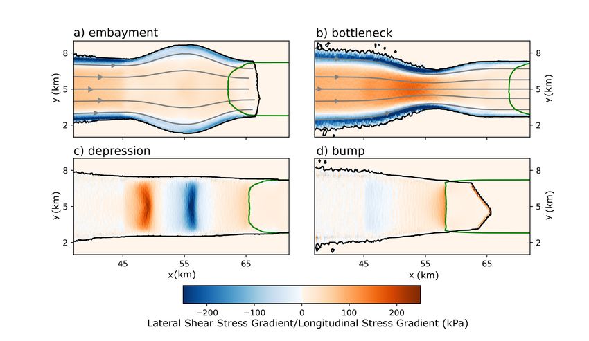
582                                                          T. Frank et al.: Geometric controls of tidewater glacier dynamics

1992; Carr et al., 2013; Bunce et al., 2018; Catania et al.,         are limited in space and time. While remotely sensed obser-
2018), Svalbard (Schuler et al., 2020), Novaya Zemlya (Carr          vations of ice dynamics over the past decades exist, the re-
et al., 2014) and North America (McNabb and Hock, 2014)              cent retreat in Greenland and elsewhere over this period is too
as well as in Antarctica (Pattyn and Morlighem, 2020). Even          short to allow for a complete assessment of geometry–glacier
adjacent glaciers with similar climatic and oceanic condi-           interactions (Carr et al., 2013; Catania et al., 2018; Bunce
tions can show strongly different behavior (Carr et al., 2013;       et al., 2018). In contrast, on paleo-timescales, retreat has oc-
Catania et al., 2018; Bunce et al., 2018). The main proposed         curred over large distances, but the temporal resolution of
explanation is that differing bathymetry and glacier geome-          geomorphological studies is limited by the available geolog-
try significantly modulate glacier response to climate over a        ical data, and key information is missing to discern different
range of timescales (Warren and Glasser, 1992; Briner et al.,        drivers of glacier retreat (Briner et al., 2009; Åkesson et al.,
2009; Jamieson et al., 2012; Åkesson et al., 2018a; Cata-            2020). Meanwhile, numerical studies that can address these
nia et al., 2018). Broadly, there is a consensus that wide and       issues have so far mostly used width- and depth-integrated
deep parts of a fjord promote retreat, while narrow and shal-        flow line models, which carry many assumptions that do not
low areas tend to stabilize glacier termini. Moreover, kine-         hold in some settings (Nick et al., 2009; Enderlin et al., 2013;
matic wave theory indicates that the upstream propagation            Åkesson et al., 2018b; Steiger et al., 2018). In particular, they
of a thinning signal is heavily influenced by bed topography         parameterize or do not account for factors that are thought to
(Felikson et al., 2017, 2021). Modeling of idealized settings        be instrumental to explain ice–topography interactions, such
(Enderlin et al., 2013; Åkesson et al., 2018b) and theoretical       as lateral drag, across-flow variations in glacier characteris-
studies based on analytical calculations and numerical exper-        tics and viscosity changes due to variations in ice tempera-
iments further emphasize the potential of fjord geometry to          ture. The latter, for instance, was found to be key to explain
modulate glacier retreat (Weertman, 1974; Raymond, 1996;             Jakobshavn Isbræ’s recent retreat (Bondzio et al., 2017).
Vieli et al., 2001; Schoof, 2007; Pfeffer, 2007; Gudmundsson            Here, we use a numerical ice-flow model resolving two
et al., 2012; Gudmundsson, 2013).                                    horizontal dimensions; we include a suite of 21 experiments
   It is therefore critical to advance our understanding of the      and present a systematic approach to compare the relative im-
influence of fjord geometry on glacier retreat to accurately         portance of basal and lateral fjord topography. This setup al-
predict sea-level rise, especially when extrapolating observa-       lows the assessment of how fjord topography controls glacier
tions of a few well-monitored glaciers to those less studied         retreat on interannual to centennial timescales. We hypothe-
(Nick et al., 2009). This knowledge is also pivotal to cor-          size that there are quantifiable relationships between glacier
rectly infer past climate signals from glacier proximal land-        retreat and topography that apply to a wide range of glacio-
forms because their formation may have been influenced by            logical settings. Such general relationships would yield sub-
fjord topography and may not necessarily have been in equi-          stantial predictive power for a broad assessment of expected
librium with the prevailing climate (Åkesson et al., 2018b;          future outlet glacier retreat.
Steiger et al., 2018).                                                  We create a large ensemble of artificial fjords that include
   The most important suggested mechanisms behind geo-               geometric features (referred to as “perturbations” in the fol-
metric control of glacier retreat are (1) friction, with glaciers    lowing) typically found in glacial fjords, such as sills and
in narrow fjords and grounded well above flotation being             overdeepenings (referred to as “bumps” and “depressions”,
stabilized by fjord geometry, while the opposite is the case         respectively; together “basal perturbations”) as well as nar-
for glaciers in wide fjords and close to flotation (Raymond,         row and wide fjord sections (referred to as “bottlenecks”
1996; Pfeffer, 2007; Enderlin et al., 2013; Åkesson et al.,          and “embayments”, respectively; together “lateral perturba-
2018b) (buttressing and lateral shear between an ice shelf           tions”). We then force synthetic glaciers to retreat through
and nearby islands and/or fjord walls can be an important            this variety of fjords by increasing ocean-induced melt rates
factor as well; Gudmundsson et al., 2012; Gudmundsson,               and assess key retreat metrics such as the grounding line re-
2013; Jamieson et al., 2012, 2014); (2) area exposed to ocean        treat rate. The ice dynamics of each simulation are compared
melt, where a wider or deeper fjord induces a larger cumu-           and quantitatively linked to the characteristics of the respec-
lative melt flux (Straneo et al., 2013; Åkesson et al., 2018b);      tive fjord geometry. Finally, we investigate whether the re-
and (3) the marine ice sheet instability (MISI), which is a          treat dynamics and ice–topography interactions are transfer-
feedback mechanism between increasing driving stress with            able from the idealized setup to a long-term study on Jakob-
increasing ice thickness at the grounding line (GL), where           shavn Isbræ in western Greenland.
inland-sloping (retrograde) beds lead to self-accelerating ice
loss (Weertman, 1974; Schoof, 2007).
   While the main controls of ice–topography interactions are
known, a quantitative understanding is still largely missing,
especially on timescales beyond a few decades. In this con-
text, in situ observations of ice dynamics do not cover the
full spectrum of ice–topography interactions because they

The Cryosphere, 16, 581–601, 2022                                                         https://doi.org/10.5194/tc-16-581-2022
T. Frank et al.: Geometric controls of tidewater glacier dynamics                                                               583

2     Methods                                                       as N = ρi gH − ρw gmax(0, −zB ), where ρi and ρw are the
                                                                    density of ice and salt water, respectively; g is gravitational
2.1    Ice sheet model                                              acceleration; H is ice thickness; and zB is bed elevation with
                                                                    respect to sea level. N is thus the difference between the ice
We use the Ice-sheet and Sea-level System Model (ISSM;              overburden and water pressure assuming perfect connectiv-
Larour et al., 2012) with the shallow-shelf approximation           ity between the subglacial water layer and the ocean. The
(SSA; Morland, 1987; MacAyeal, 1989). A discussion on               effective pressure in the friction law induces an elevation de-
the appropriateness of this approximation compared to a full-       pendence of the basal resistance to flow. This dependence is
Stokes model is provided in Sect. 4.2. Our domain is rectan-        motivated through the assumption that weak sediments are
gular (80 km × 10 km), with x and y representing the along-         more likely to be present in low-lying areas. Implications for
flow and across-flow coordinates, respectively (Fig. 1a). We        our results are discussed in Sect. 4.2. We set k as spatially
create an unstructured mesh with a fixed resolution of 100 m        uniform to isolate the topographic signal of retreat in our re-
close to the GL, comparable to other high-resolution studies        sults and thus to reduce the number of degrees of freedom for
of Greenlandic fjords (e.g., Morlighem et al., 2016, 2019).                                                         1
                                                                    the interpretation. We fix k = 40 (Pa yr m−1 ) 2 , which is mid-
The temporal resolution is set to 1t = 0.01 yr (3.65 d)
                                                                    range among values typically found in glaciological settings
to satisfy the Courant–Friedrichs–Levy condition (Courant
                                                                    resembling ours (Bondzio et al., 2017; Haubner et al., 2018;
et al., 1928). We apply a subelement GL migration scheme
                                                                    Åkesson et al., 2018a).
(Seroussi et al., 2014) and enable a moving calving front with
                                                                       Ocean-induced melting is parameterized through pre-
the level-set method (Bondzio et al., 2016). We use a thermal
                                                                    scribed melt rates that are invariant of depth. On all elements
model (Larour et al., 2012) to constrain the ice rheology pa-
                                                                    that have a floating section, a fixed basal melt rate is applied,
rameter, B, based on the temperature-dependent relationship
                                                                    thinning the ice from below. The reference forcing for this
from Cuffey and Paterson (2010). The spin-up ice temper-
                                                                    subshelf melt rate used for model spin-up is 30 m yr−1 . All
ature is −5 ◦ C, representative of conditions in southern and
                                                                    elements at the ice front are subject to a frontal rate of un-
central Greenland and the southern Fennoscandian Ice Sheet
                                                                    dercutting if they are grounded. This parameterization ac-
(Nick et al., 2013; Åkesson et al., 2018a). To simulate calv-
                                                                    counts for both small-scale calving events associated with
ing, a von Mises law is used (Morlighem et al., 2016), where
                                                                    undercutting and direct melt at the ice front (Rignot et al.,
the calving rate c is given as
                                                                    2016; Morlighem et al., 2019). The reference forcing here
             σ̃                                                     is 200 m yr−1 . Both values are on the lower end of observed
c = ||v||        ,                                           (1)    melt rates (Motyka et al., 2003; Enderlin and Howat, 2013;
            σmax
                                                                    Xu et al., 2013), thus reflecting a configuration prior to re-
where v is the velocity vector, σ̃ is a scalar quantity rep-        cent warming when glaciers were more in balance with the
resenting the tensile stress at the ice front, and σmax is a        ambient climate than today (King et al., 2020). For both fric-
stress threshold. This formulation, demonstrated to perform         tion and melt, experiments not shown here indicate that the
well in Greenlandic fjords (Choi et al., 2018), means that ice      mesh is sufficiently refined in the vicinity of the grounding
front retreat occurs when the tensile stress at the glacier front   line so that the type of subelement scheme chosen does not
exceeds a fixed threshold; σmax generally needs to be de-           affect the simulations significantly.
termined experimentally for studies on real-world glaciers.            As part of the idealized setup, the surface mass balance
Here we fix σmax to 1 MPa for grounded ice and 200 kPa              (SMB) is fixed to zero, except in the uppermost 10 km of
for floating ice. These values yield a representative setup and     the domain (Fig. 1a), where we set an accumulation rate of
are within the range suggested for Greenland outlet glaciers        55 m yr−1 . This creates a realistic fixed upstream ice flux and
(Morlighem et al., 2016; Choi et al., 2018, 2021). Note that        is not meant to represent local SMB found on real glaciers.
the choice of the calving law is an important yet poorly con-       Additionally, mass is added to the model domain by fixing an
strained control on the grounding line dynamics and ice front       ice velocity of vx = 50 m yr−1 at the upper domain boundary,
behavior (Schoof et al., 2017; Haseloff and Sergienko, 2018).       which creates an influx as a function of the glacier thickness.
In the absence of a universal calving law, a reasonable as-         These two approaches to adding mass represent a total accu-
sumption has to be made, and we justify the choice of the           mulation (A) which can be expressed as
von Mises law through its relatively good performance in                      yZmax
real-world applications (Choi et al., 2018).
   Basal sliding is parameterized with a Budd-type friction         A=C+           vx (0, y) H (0, y) dy,                        (3)
law (Budd et al., 1984) of the form                                            0
                                                                                           2
τ b = −k 2 Nv b ,                                            (2)    where C = 10 × 103 × 55 = 5.5 × 10⁹ m3 yr−1 is a con-
                                                                    stant accumulation. Through the thickness-dependent influx
where τ b is basal drag, k is a friction parameter, v b is the      represented by the second term on the right-hand side, we ac-
basal velocity, and N is the effective pressure. N is given         count for a reduction in accumulation for a shrinking glacier,

https://doi.org/10.5194/tc-16-581-2022                                                       The Cryosphere, 16, 581–601, 2022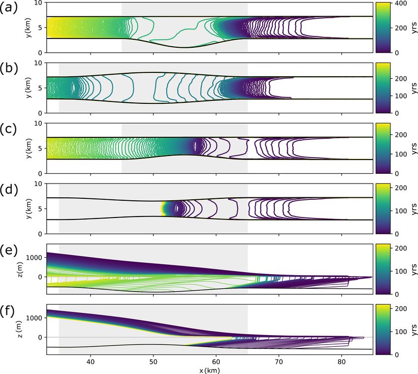
584                                                           T. Frank et al.: Geometric controls of tidewater glacier dynamics

thus parameterizing the SMB–altitude feedback (Harrison               that y20 − y10 is the width of the outlet channel in a trans-
et al., 2001; Oerlemans and Nick, 2005).                              formed coordinate system that is oriented such that the co-
   We impose free-slip boundaries at the lateral margins of           ordinates (x 0 , y 0 ) are parallel and perpendicular to the center
the domain (where y = 0 and y = ymax ), meaning that no               line of the outlet channel, respectively, at any given point. S
mass can leave the system laterally. In summary, the only             combines information about the width and depth of a fjord
mass source is at the upstream end of the domain, while the           and is thus a comprehensible parameter for comparing basal
only mass wasting occurs where the glacier is in contact with         and lateral perturbations. Furthermore, it is straightforward
                                                                                                           dS
the ocean (through either calving or melting).                        to calculate its first derivative dx   0 (in the following written as
                                                                      dS for brevity), which yields information on the along-fjord
2.2   Fjord geometries                                                change in width and/or depth.
                                                                         Besides our reference setup, we test 20 fjord geometries
Our reference geometry is a fjord sloping linearly towards            (Table 2, Fig. 2), each of which contains either a small,
the ocean with a wide section in the upstream area from               medium or large geometric perturbation. The magnitude of
which ice is funneled towards a 5 km wide outlet channel              the perturbation is defined by how much the width or depth
with parallel walls (Fig. 1a). The fjord topography is given          of the fjord deviates from the reference fjord. Our “core ex-
by B(x, y) = Bx (x) + By (x, y) with                                  periment”, which the results focus on, comprises 12 fjords,
Bx (x) = B0 + x × α + 2(x)                                    (4)     each of which features one of the four perturbation types (de-
                                                                      pression, bump, bottleneck, embayment) of one of the three
and                                                                   magnitude classes (small, medium, large). The depressions
                                  df − Bx (x)                         and embayments in each magnitude class increase the wet-
By (x, y) =                                                       ted area S at the center of the perturbation xC by the same
                              mf y− 12 Ly +wf +(x)+2(x)
                   1+e                                                amount, while the bottlenecks and bumps in each magnitude
                                df − Bx (x)                           class reduce S at xC by the same amount. The along-flow
            +                                         ,   (5)     horizontal extent of all perturbations in the core experiment
                           −mf y− 21 Ly −wf −(x)−2(x)
                  1+e                                                 is 20 km (Fig. 2).
                                            2                            In the eight simulations outside our core experiments, we
where (0 < x < xU ) = x−x     F
                                 U
                                    . The parameter values and        test asymmetric and longer perturbations to verify if the
descriptions are found in Table 1. This formulation is in-            results from our core experiment can be transferred to a
spired by the Marine Ice Sheet Model Intercomparison                  wider range of settings. We test two asymmetric embay-
Project (MISMIP) setup (Gudmundsson et al., 2012; Asay-               ments, which have the same S at xC as the small and medium
Davis et al., 2016) but adapted to our purpose.                       embayments and depressions, as well as two asymmetric bot-
   To insert basal or lateral perturbations in the outlet channel     tlenecks, which have the same S at xC as the small and large
and thus alter the fjords’ depth or width in specific areas, we       bottlenecks and bumps. The longer perturbations have an
modify the parameter 2(x) in either Eq. (4) or Eq. (5) such           along-flow horizontal extent of 30 km. We test one longer
that                                                                  perturbation per perturbation type with S at xC correspond-
                                                                      ing to the medium magnitude class.

                               2π        3           0 0
2(xB < x < xE ) = − sin              x − − xC           + . (6)
                               3         4           2 2
Altering 2(x) in only one of the terms on the right-hand              2.3   Reference glacier
side of Eq. (5) allows fjords to be produced with one-sided
lateral perturbations, thus making them asymmetric. Com-              All experiments start from an artificial reference glacier,
bined, these equations reproduce the typical U shape of fjords        which is produced by relaxing a rectangular block of ice
(Fig. 1b) and yield a setting that is representative of a wide        in the reference fjord. The spin-up is run until the rela-
range of outlet glaciers.                                             tive ice volume ((dV /yr)/V  0.05 %) and GL position are
   The metric used to quantitatively link fjord shape with            steady. The length of the spun-up reference glacier is 82 km,
glacier retreat is the wetted area S: the submerged cross-            its GL is at x = 73 km, and the velocity at the GL along
sectional area of the fjord (Fig. 1b), which can be calculated        the central flow line of the glacier vGL = 2.5 km yr−1 . In
at any point along an outlet channel according to                     a steady state, the total mass gain is ∼ 6.1 km3 yr−1 (≈
              0                                                       5.6 Gt yr−1 ), which is balanced by mass losses through melt-
            Zy2                                                       ing at the ice–ocean interface (∼ 0.9 km3 yr−1 ) and calving
S(x 0 ) =         D(x 0 , y 0 )dy 0 ,                         (7)     (∼ 5.2 km3 yr−1 ). In a sensitivity experiment with doubled
            y10                                                       ocean melt rates (400 m yr−1 undercutting and 60 m yr−1
                                                                      subshelf melting), mass loss through ocean melt increases to
where D is the water depth, and y10 and y20 are the intersec-         ∼ 2.1 km3 yr−1 , while calving reduces to ∼ 4 km3 yr−1 . The
tions of the water line in the fjord with the fjord walls so          GL remains largely unchanged, indicating that the reference

The Cryosphere, 16, 581–601, 2022                                                           https://doi.org/10.5194/tc-16-581-2022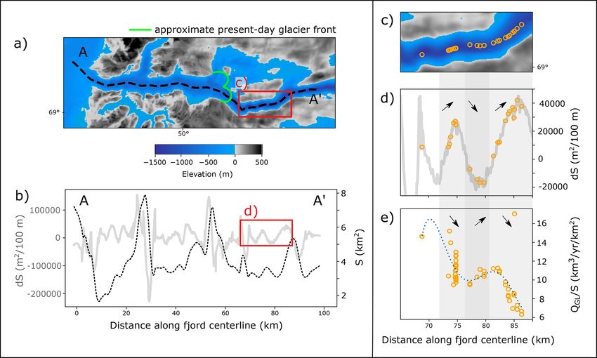
T. Frank et al.: Geometric controls of tidewater glacier dynamics                                                                           585

Figure 1. Schematic of the experimental setup. (a) Sketch of the domain (not to scale) with annotated dimensions and mass balance processes
(gains: thickness-dependent influx and surface accumulation; losses: melt at the ice–ocean interface and calving). The red box symbolizes
how the fjord geometry is changed in different experiments to include geometric perturbations (their center being referred to as xC ). (b) Cross-
sections through the linear fjord (black line) and geometric perturbations. Upper panel: basal perturbations (green: depression; gray: bump);
lower panel: lateral perturbations (blue: embayment; yellow: bottleneck). The wetted area, i.e., the cross-sectional area of the fjord below sea
level, is shaded in blue for each geometry.

Table 1. Parameters for generating fjord geometries (in parentheses for longer geometric perturbations).

                Parameter        Value    Unit    Description
                B                         m       Bed elevation
                B0              −450      m       Bed elevation at x = 0
                α              −0.002             Slope of bed in x direction
                df               2000     m       Depth of fjord relative to upland areas on the sides
                Ly                 10     km      Width of domain in y direction
                Lx                 85     km      Length of domain in x direction
                wf                 2.5    km      Half-width of fjord
                mf                  1             Factor for steepness of fjord walls
                                   300
                xU                  30    km      Extent in x direction of wide upstream area
                F                 300             Factor for smooth transition between wide upstream area and parallel fjord
                xB             45 (35)    km      x coordinate of upstream end of perturbation
                xE             65 (65)    km      x coordinate of downstream end of perturbation
                xC             55 (50)    km      x coordinate of center of perturbation
                3              20 (30)    km      Horizontal extent of perturbation in x direction
                0             Variable    m       Deviation in fjord half-width or depth relative to parallel fjord at xC

glacier is not very sensitive to ocean forcing due to compen-              2.4   Retreat experiments in variable fjords
sating effects in the mass wasting processes.
   The setup represents a medium-sized fjord–glacier system,
which has similar dimensions and dynamics as, for example,                 We slightly modify the reference glacier to match the new
the present-day Alison glacier in NW Greenland, where the                  fjord geometry when introducing geometric perturbations.
fjord width is about 5 km, water depth is around 500 m, and                For embayments, we extrapolate the glacier surface laterally
observed ice discharge has increased from ∼ 4 to ∼ 8 Gt yr−1               to fill the newly introduced lateral cavities. For depressions,
in the past 20 yr (Mouginot et al., 2019). It is furthermore               we fill the new basal cavity with ice but keep the glacier
broadly representative of outlet glaciers from the Fennoscan-              surface the same. For bumps or bottlenecks, we remove ice
dian Ice Sheet during the last glacial, such as the Hardanger-             while keeping the glacier surface unaltered. Subsequently,
fjorden glacier (Mangerud et al., 2013; Åkesson et al., 2020).             we relax the glacier in each geometry for 50 yr, resulting in

https://doi.org/10.5194/tc-16-581-2022                                                                The Cryosphere, 16, 581–601, 2022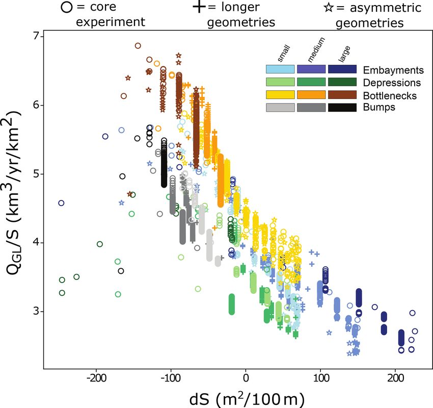
586                                                                T. Frank et al.: Geometric controls of tidewater glacier dynamics

Table 2. Suite of experiments with name (extensions _lon and _asy refer to longer and asymmetric geometries), type of geometric perturba-
tion, perturbation magnitude, the deviation in fjord width (2 0 for symmetric lateral perturbations, 1 0 for asymmetric ones) or depth (1 0
for basal perturbations) at the center of the perturbation relative to the linear reference fjord, S at xC (i.e., the wetted area at the center of the
perturbation), and forcings required to induce complete retreat through the entire geometric perturbation (/ if no complete retreat could be
enforced).

      Experiment          Perturbation     Perturbation     Fjord width or depth      S at xC                  Forcing for complete retreat
                          type             magnitude               deviation [m]       [km2 ]    (undercutting/subshelf melt rate) [m yr−1 ]
      Ref                 –                –                                   0          2.1                                        800/120
      ByH450              Embayment        Small                             900          2.6                                       1200/180
      ByH900              Embayment        Medium                           1800          3.1                                       1200/180
      ByH1350             Embayment        Large                            2700          3.6                                       1200/180
      ByH-450             Bottleneck       Small                            −900          1.6                                        800/120
      ByH-675             Bottleneck       Medium                          −1350          1.3                                              /
      ByH-900             Bottleneck       Large                           −1800          1.1                                              /
      BuH-120             Depression       Small                            −120          2.6                                       1200/180
      BuH-240             Depression       Medium                           −240          3.1                                       1000/150
      BuH-360             Depression       Large                            −360          3.6                                        800/120
      BuH120              Bump             Small                             120          1.6                                              /
      BuH180              Bump             Medium                            180          1.3                                              /
      BuH240              Bump             Large                             240          1.1                                              /
      ByH900_lon          Embayment        Medium                           1800          2.8                                       1200/180
      ByH-675_lon         Bottleneck       Medium                          −1350          1.5                                       1200/180
      BuH-240_lon         Depression       Medium                           −240          2.8                                       1200/180
      BuH180_lon          Bump             Medium                            180          1.5                                              /
      ByH900_asy          Embayment        Small                             900          2.6                                       1200/180
      ByH1800_asy         Embayment        Medium                           1800          3.1                                       1200/180
      ByH-900_asy         Bottleneck       Small                            −900          1.6                                       1200/180
      ByH-1800_asy        Bottleneck       Large                           −1800          1.1                                              /

an ice volume change (dV /yr)/V < 0.5 % at the end of re-                    treat rate, dGL), the front position (xFr ) and its derivative (the
laxation for every setup tested and a steady GL.                             frontal retreat rate, dFr), and also the velocity at the GL (vGL )
   After relaxation, we increase the ocean forcing to trigger a              and the shelf length (LS ) are measured along the central flow
retreat. We aim to force the GL to retreat through the entire                line of the glacier.
geometric perturbations. The ocean melt rates required to in-
duce such a retreat depend on the fjord geometry, which we                   2.5    A real-world case study: Jakobshavn Isbræ
elaborate on in the results section. To determine what melt
rates are needed to force this complete retreat in a partic-
                                                                             We want to verify the degree to which the dynamics seen
ular fjord, we strengthen the ocean forcing using multiples
                                                                             in our experiments are also prevalent in real-world settings.
of the reference forcing (200 m yr−1 frontal rate of under-
                                                                             This is challenging since we investigate decadal to centennial
cutting, 30 m yr−1 subshelf melt) until complete retreat takes
                                                                             timescales. Specifically, we would need observations with
place. In some cases (cf. Sect. 3.2), even unrealistically high
                                                                             high temporal resolution on glacier metrics (Table 3) for a
values for the ocean forcing (e.g., 20 times the reference forc-
                                                                             glacier that has retreated over tens of kilometers through a
ing) did not trigger complete retreat, suggesting that glaciers
                                                                             fjord with variable and known topography. There are perhaps
in these geometries are not sensitive to ocean melt.
                                                                             only a handful of glaciers worldwide that may fulfill these
   Since we want to explore the response of outlet glaciers to
                                                                             requirements, and even so, acquiring the necessary data is
melting at the ice–ocean interface, we keep the SMB constant
                                                                             difficult and outside the scope of the present study.
with time and let the upstream ice flux vary only through our
                                                                                To test our idealized results in a real-world setting, we in-
parameterized SMB–altitude feedback (Eq. 3).
                                                                             stead turn to model simulations from the evolution of Jakob-
   We assess 16 glacier metrics during the retreat, which we
                                                                             shavn Isbræ (JI) in the Holocene (Kajanto et al., 2020). We
expect to show a response to local topography (Table 3). All
                                                                             focus on an 8000-year simulation of the retreat of JI from a
of these can be observed in situ or via remote sensing tech-
                                                                             sill at the fjord mouth of Jakobshavn Isfjord to a point in-
niques (e.g., Mouginot et al., 2019; King et al., 2020), which
                                                                             land of today’s GL position. This model retreat is forced us-
means that our results are readily transferable to real-world
                                                                             ing a step reduction in the equilibrium line altitude early in
settings. The GL position (xGL ) and its derivative (the GL re-
                                                                             the Holocene (experiment SE_CM in Kajanto et al., 2020).

The Cryosphere, 16, 581–601, 2022                                                                    https://doi.org/10.5194/tc-16-581-2022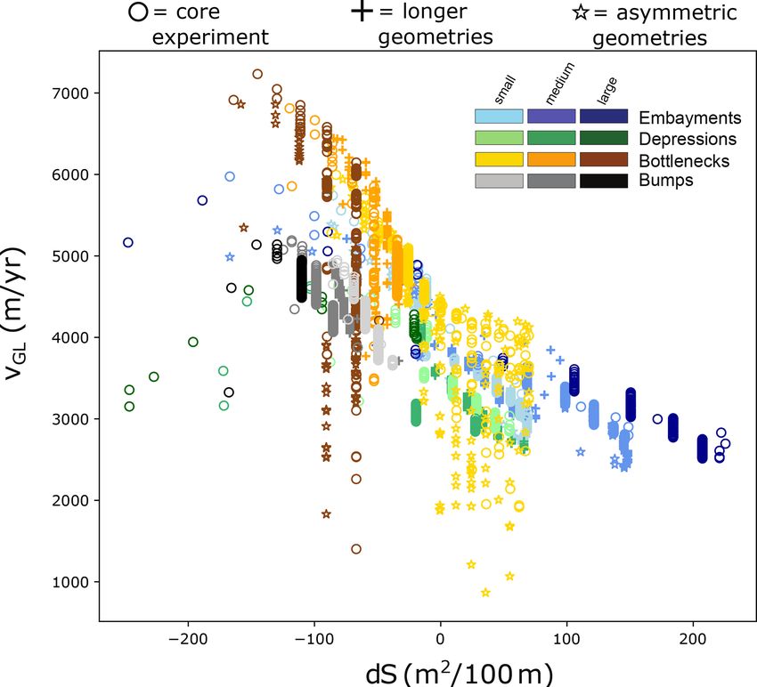
T. Frank et al.: Geometric controls of tidewater glacier dynamics                                                                          587

Figure 2. Along-fjord profiles of the wetted area S (a: lateral; b: basal perturbations) and its derivative dS (c: lateral; d: basal) for fjords
featuring different geometric perturbations of different magnitude classes. Note that the profiles of embayments and depressions and likewise
bottlenecks and bumps of the same magnitude class are largely congruent, thus allowing a straightforward comparison between basal and
lateral perturbations.

Table 3. Glacier characteristics assessed during retreat for later cor-      Just like in our idealized experiments, we calculate S and
relation with fjord geometry. Parameters marked with ∗ are assessed       dS for Jakobshavn Isfjord. We then assess whether the rela-
along the central flow line of the glacier.                               tionships found in our idealized settings are also prevalent in
                                                                          JI’s dynamics (Sect. 3.5).
      Glacier metric                      Variable    Unit
      Grounding line position∗            xGL         km
                                                                          3     Results
      Grounding line retreat rate∗        dGL         m yr−1
      Front position∗                     xFr         km                  3.1    Stagnant and ephemeral grounding line positions
      Front retreat rate∗                 dFr         m yr−1
      Grounding line mass flux            QGL         km3 yr−1            We identify positions of GL stagnation (“stagnant” GL posi-
      Ice front mass flux                 QFr         km3 yr−1            tions), i.e., where the GL rests for a sustained time (typically
      Flux through an upstream gate       QU          km3 yr−1            50 to 200 years) or retreats slowly (dGL > −100 m yr−1 ),
      Calving flux                        QC          km3 yr−1            and areas where the GL retreats quickly (“ephemeral” GL
      Velocity at the grounding line∗     vGL         m yr−1              positions; dGL < −500 m yr−1 ). Figure 3 shows both stag-
      Maximum velocity                    vmax        m yr−1              nant and ephemeral positions for one representative run per
      Shelf length∗                       LS          m
                                                                          perturbation type. For a comparison of the GL retreat dynam-
      Floating area                       AF          m2
                                                                          ics of all simulations within our core experiment, the reader
      Grounded area                       AG          m2
                                                                          is referred to Fig. A1. Note that in the following, all termi-
      Ice volume                          V           km3
                                                                          nology related to along-fjord changes in width or depth of
      Ice volume above flotation          VAF         km3
      Maximum ice thickness               Hmax        m
                                                                          the fjord (e.g., narrowing, deepening) refers to the direction
                                                                          of glacier retreat.
                                                                             Stagnant positions exist at the downstream end of em-
                                                                          bayments and depressions where the fjord becomes wider
While this is a sensitivity experiment not meant to reflect the           and deeper (x ≈ 62 to 65 km; Fig. 3a, c). Ephemeral po-
actual evolution of JI (Kajanto et al., 2020), it is convenient           sitions, associated with rapid retreat, are found in the re-
for our purposes since it produces a long-lasting, dynamic                mainder of both perturbations (x ≈ 45 to 62 km). Retreat
retreat.                                                                  from the stagnant position at the downstream end of the em-

https://doi.org/10.5194/tc-16-581-2022                                                               The Cryosphere, 16, 581–601, 2022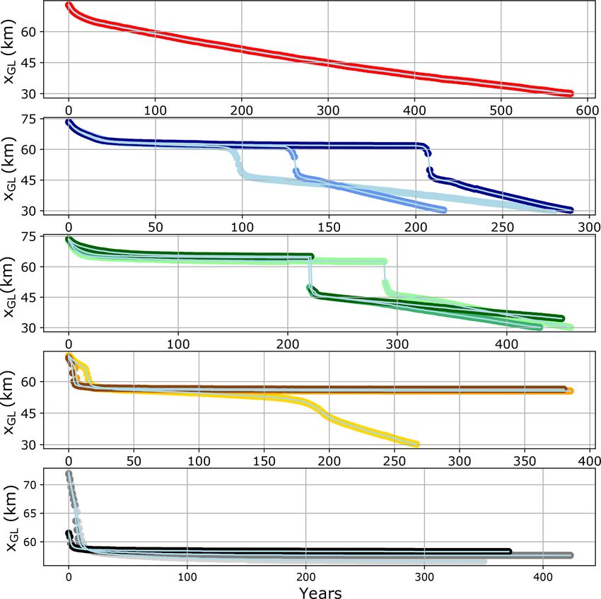
588                                                          T. Frank et al.: Geometric controls of tidewater glacier dynamics

bayment occurs gradually (dGL ≈ −22 m yr−1 , while xGL ≈             This increase is larger than what is needed to induce retreat
62 to 64 km) but is rapidly accelerating as the GL retreats fur-     through the linear reference fjord (4 times the spin-up forc-
ther into the perturbation, accompanied by some lateral un-          ing). The residence time of the GL in the stagnant positions
grounding. Retreat from the stagnant position in the depres-         at the downstream end of the embayments is such that the
sion occurs suddenly after a phase of near-stability (dGL ≈          glacier in the smallest embayment is the earliest to retreat
−6 m yr−1 , while xGL ≈ 64.5 to 65.5 km) as the glacier un-          (after 61 yr of GL stagnation), and the one in the largest is
grounds where the fjord is deepest in the center of the pertur-      the latest (after 173 yr) (Fig. 4). This implies that the larger
bation (x ≈ 55 km; Fig. 3c inset plot). The cavity formed un-        the embayment, the more stability it provides to the glacier at
der the glacier rapidly grows in size and expands downstream         its downstream end before retreat through the entire pertur-
until it eventually detaches the glacier from the bed also at        bation is possible. A larger embayment means a locally larger
the downstream end of the depression (x ≈ 65 km). In bot-            along-flow change in wetted area dS at its downstream end
tlenecks and on bumps, stagnant positions are found where            (Fig. 2). Thus, there is a positive correlation between GL sta-
the fjord is narrow and shallow (x ≈ 55 to 58 km; Fig. 3b,           bility and dS. This indicates that dS not only determines the
d). The stabilizing effect of bumps is, in fact, so large that       location of stagnant GL positions in embayments, as shown
no glacier could be forced to retreat over them within rea-          before, but that it also quantitatively impacts how stagnant
sonable limits for the ocean forcing. However, we observe            the GL is.
that retreat onto bumps occurs fast (dGL ≈ −500 m yr−1 for              The glaciers in fjords with depressions require different
xGL ≈ 58 to 65 km). For bottlenecks, only the glacier situ-          forcings to retreat completely (small: 6× the reference forc-
ated in the fjord with a “small” bottleneck (i.e., the bottleneck    ing; medium: 5×; large: 4×). The residence time also varies;
with the largest S among the ones tested) could be forced to         retreat over small depressions occurs ∼ 65 yr later than over
retreat completely. Noticeably, retreat at the downstream end        medium and large depressions, which retreat after about the
of the bottleneck (x ≈ 56 to 65 km), where the fjord narrows         same time (after 169 and 170 yr, respectively). These findings
in, is fast (ephemeral), with dGL ≈ −900 m yr−1 , whereas it         indicate that the stabilizing effect of a depression declines the
is very slow (relatively stagnant), with dGL ≈ −25 m yr−1 ,          deeper it is (Fig. 4). Thus, there is a negative correlation be-
upstream of the narrowest point, where the fjord is widening         tween GL stagnation and S. In Sect. 3.1, ungrounding in the
(x ≈ 45 to 55 km; Fig. 3d).                                          central part of depressions was identified as the trigger of
   In summary, stagnant GL positions are found where the             rapid retreat from the temporary stillstands. Such GL retreat
fjord widens and deepens in the direction of glacier retreat         occurs more easily in a deeper fjord (larger S). Therefore,
(positive dS; Fig. 2), and rapid retreat occurs through areas        it is consequential that a deeper depression is less stabiliz-
where the fjord becomes narrower and shallower (negative             ing. Note, however, that the fjord depth several kilometers
dS). Thus, the along-fjord change in width or depth (dS) is          upstream of the GL determines how long the GL stagnates.
a key control on GL retreat. However, glaciers in narrower           There is no direct correlation between S or dS at the GL and
or shallower fjords than the reference fjord (bottlenecks and        the stability provided to the glacier by the fjord in our settings
bumps) can also temporarily stagnate where S is small. This          with depressions.
shows that the wetted area constitutes an additional important          The glacier in a fjord with a “small” bottleneck required
control on GL retreat. The experiments with asymmetric and           a 4-fold increase in oceanic melt rates and retreated from its
longer perturbations confirm these findings (see Fig. A2).           stagnant position after 126 yr of stagnation. This is a weaker
                                                                     forcing than for the glaciers in the embayments as well as
3.2   Forcings and timings of retreat                                for the medium and small depressions and thus suggests that
                                                                     this bottleneck provides less stability than these geometries.
Now, we investigate how retreat from stagnant and                    This contrasts with the common pattern, where a small S and
ephemeral GL positions is correlated with fjord topography           a positive dS should stabilize the glacier strongly. It is un-
(i.e., S and dS). Two parameters are important in this con-          clear why this is the case here. We hypothesize that it might
text (Fig. 4): first, the amplitude of the forcings needed to        be related to a combination of high driving stresses due to a
induce complete retreat through the different geometric per-         steepened surface inside the bottleneck in conjunction with
turbations. As mentioned previously, distinctions exist be-          high modeled calving rates (not shown). The two experi-
tween both the different perturbation types (bumps, depres-          ments with glaciers in geometries with narrower bottlenecks
sions, bottlenecks, embayments) and the different magnitude          (“medium” and “large” bottleneck) did not retreat through
classes (small, medium, large) for a given geometry type.            the entire perturbation. This, in turn, aligns well with the
The second important parameter is the approximate resi-              general notion of a confined (low S) and downstream narrow-
dence time of the GL in a stagnant position. The stronger            ing (positive dS) fjord yielding strong stability to the glacier.
the GL is stabilized by a particular geometric perturbation,         Likewise, none of the glaciers in fjords with bumps retreated
the longer it will be stagnating.                                    completely, which follows the same concept. However, the
   All glaciers in embayments require the same increase in           strong stability that bumps provide to the glacier may also be
forcing to retreat completely (6 times the spin-up forcing).         related to the choice of model parameters (Sect. 4.2).

The Cryosphere, 16, 581–601, 2022                                                         https://doi.org/10.5194/tc-16-581-2022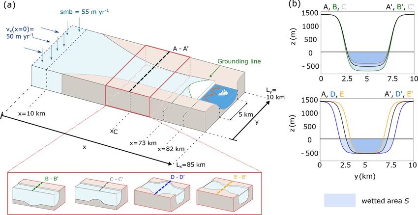
T. Frank et al.: Geometric controls of tidewater glacier dynamics 589
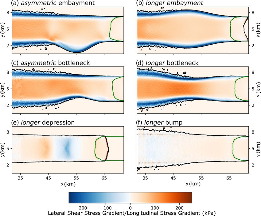
Figure 3. Annual glacier evolution (a, b: top-down view of domain showing yearly grounding lines; c, d: yearly glacier profiles along central
flow line) in fjords featuring different geometric perturbations (location of perturbations marked in gray) with the spacing between the lines
indicating retreat velocity: (a) medium embayment, (b) small bottleneck, (c) medium depression, (d) small bump. Inset plot in (c) shows
profile (blue) in year 217 when glacier ungrounds in the central part of the depression, which triggers further retreat. The red line is the level
to which a glacier needs to thin to reach flotation.
3.3 Stress balance response to fjord geometry found where ice is funneled in a downstream narrowing fjord.
This occurs, for example, where 55 km < x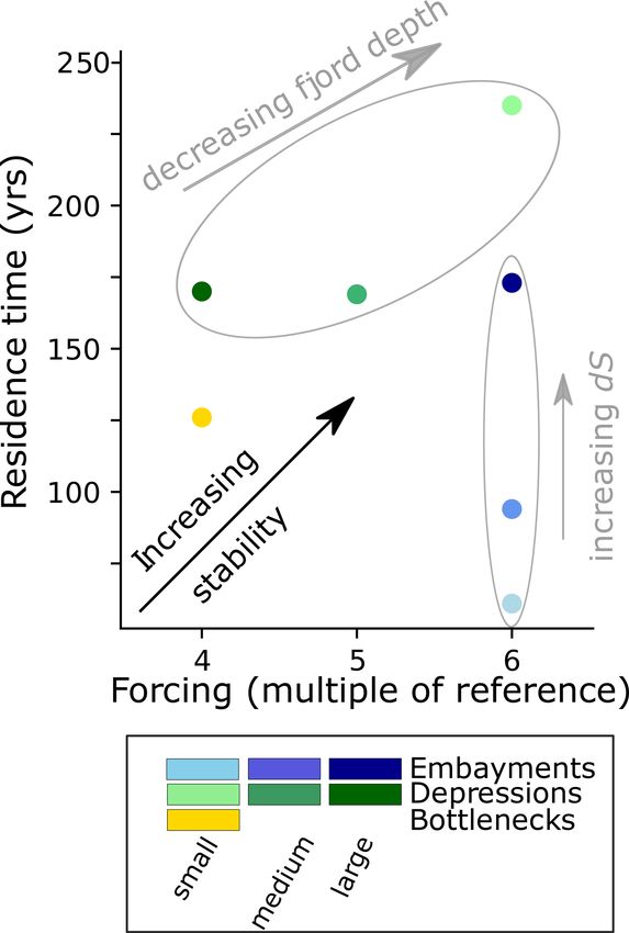
590                                                             T. Frank et al.: Geometric controls of tidewater glacier dynamics

                                                                        3.4   A quantitative relationship for ice–topography
                                                                              interaction

                                                                        We hypothesize that there is a quantitative relationship be-
                                                                        tween fjord geometry and glacier retreat, valid across a range
                                                                        of different geometries. To test this, we correlate a variety
                                                                        of metrics indicative of glacier retreat (Table 3) against rele-
                                                                        vant metrics of fjord geometry, that is, the submerged cross-
                                                                        sectional area (S) and its derivative (dS). We restrict the data
                                                                        to those instances when the GL is located within a geometric
                                                                        perturbation (gray-shaded areas in Fig. 3). Among all com-
                                                                        binations of retreat and geometry metrics tested, including
                                                                        those of asymmetric and “longer” perturbations (Table 2),
                                                                        the clearest and most universal relationship found is a nega-
                                                                        tive, close-to-linear correlation between the ratio of the GL
                                                                        flux and the submerged cross-sectional area QGL /S over the
                                                                        change in submerged cross-sectional area dS (Fig. 6). This
                                                                        relation expresses that a widening or deepening fjord in the
                                                                        downstream direction (negative dS) promotes a high GL flux
                                                                        per wetted area (QGL /S). Conversely, a glacier retreating
                                                                        in a fjord that becomes narrower or shallower downstream
                                                                        (positive dS) will have a reduced QGL /S. Note that the ratio
                                                                        QGL /S for basal geometry perturbations (gray to black and
                                                                        green colors in Fig. 6) is on average lower than for lateral
                                                                        geometry perturbations. This means that basal perturbations
                                                                        generally inhibit ice flux across the GL more efficiently than
Figure 4. Forcing required to induce complete retreat in multiples
                                                                        lateral perturbations (note that this may be influenced by our
of the reference forcing (200 m yr−1 undercutting rate, 30 m yr−1
                                                                        modeling choices; Sect. 4.2). Also, note that the GL flux is
subshelf melt) and approximate residence time of the GL in a stag-
nant position for different fjord geometries. A longer residence time   the product of the velocity vGL and the flux gate area at the
and a larger forcing required indicate that fjord geometry provides     GL AGL , that is QGL = vGL × AGL . The ratio QGL /S is thus
larger stability. More stability is correlated with decreasing fjord    proportional to vGL when there is hydrostatic equilibrium at
depth for depressions (shades of green) and with increasing along-      the GL (because in that case, S = 0.9 × AGL ), and so we find
fjord change in wetted area dS for embayments (shades of blue).         a comparable, negative linear relationship between vGL and
The simulations for which no retreat through the perturbation was       dS (Fig. A4).
observed have been omitted from the figure.                                 We find an additional yet less distinct negative relation-
                                                                        ship between the wetted area S and the GL retreat rate dGL
                                                                        (Fig. 7a). This shows that a wider or deeper fjord promotes
Fig. 5d). Together, the stress regimes in basal perturbations           faster GL retreat, while a narrower or shallower geometry
demonstrate that a retrograde glacier bed, tilted against the           stabilizes the glacier. This relation is not as universal as the
direction of flow, reduces longitudinal stress gradients con-           previous one since one value for dGL is not uniquely linked
siderably as it increases the basal resistance to flow, which           to one value for S across different geometries. Furthermore,
ultimately stabilizes the glacier.                                      it is not linear but rather such that for a range of low S values,
   In summary, the stress analysis above suggests that in-              dGL does not vary noticeably. Only above a certain thresh-
creased lateral shear stress gradients or negative longitudinal         old in S does the GL retreat markedly faster (Fig. 7b). This
stress gradients are found wherever ice flow is forced to con-          threshold varies between different fjord geometries. How-
verge, either horizontally or vertically, towards a narrowing           ever, we find that it is always associated with the location
or shoaling area downstream. Simulations using asymmetric               of GL stagnation (Fig. 3.1). This means that a relationship
as well as longer perturbations confirm that these findings are         between GL retreat rate dGL and S only unfolds if a local
robust (see Fig. A3). Through the convergent flow, the con-             stability position is passed. These stagnant positions can be
tact between the glacier and the fjord is enhanced, leading             either where S is low or where dS is high, as shown previ-
to increased resistance to flow. Overall, along-flow change in          ously. For instance, dGL does not increase as the GL retreats
fjord width or depth (i.e., dS) is found to define areas of in-         very slowly at the stagnant position in the downstream half
creased lateral shear gradients or negative longitudinal stress         of embayments. Only once it has retreated passed this point
gradients and thus GL stagnation.                                       of GL stagnation can a correlation between dGL and S be
                                                                        seen.

The Cryosphere, 16, 581–601, 2022                                                            https://doi.org/10.5194/tc-16-581-2022
T. Frank et al.: Geometric controls of tidewater glacier dynamics 591 Figure 5. Stress states in perturbations. Lateral shear stress gradients for (a) and (b), with flow lines in gray, and longitudinal stress gradients for basal perturbations (c, d). The green line is the grounding line; the black line is the glacier outline. For depressions we do not see a distinct relationship be- tween dGL and S (Fig. SA5). This is because we measure the GL position xGL and therefore also dGL as the farthest downstream grounded point along the central flow line of the glacier. When the glacier ungrounds in the center of a depression, where the fjord is deepest, the dynamics of re- treat are triggered several kilometers upstream of the GL, as mentioned in Sect. 3.1. Therefore, there is a correlation be- tween fjord depth and GL retreat in depressions. However, it is not reflected when only considering processes at the GL. Not finding a dGL-over-S relation for depressions is hence expected by construction of our methodology and not an ac- tual feature. 3.5 Jakobshavn Isbræ Given our previous results, we now aim to assess whether our principal geometric relationship QGL /S over dS can be found for Jakobshavn Isbræ. To this end, we calculate the wetted area S along the topography of Jakobshavn Isfjord as used in Kajanto et al. (2020), which depicts overall higher Figure 6. Relationship between grounding line discharge per wetted values and larger along-fjord changes in dS than our ideal- area QGL /S and along-fjord change in wetted area dS for all tested ized settings (Fig. 8b). geometries and all instances when the GL is within a geometric Plotting all available data points for QGL /S over dS at perturbation (gray area in Fig. 3). Jakobshavn, we do not find the aforementioned geometric re- lationship. This may have many reasons related to the com- plex dynamics of Jakobshavn Isbræ (Bondzio et al., 2017), but most critically, there is lateral inflow of ice to the main means that the rigid glacier–wall interface in our experiments channel from the surrounding ice sheet and tributaries (com- is replaced by a changing ice–ice contact. This has implica- pare with Steiger et al., 2018). This alters the stress balance tions for the lateral friction that the fast-flowing ice in the at the GL compared to our experiments, where the glacier is main channel experiences and for the processes transferring always closely confined between fjord walls. Specifically, it stabilizing back stress from the sides to the center of flow. https://doi.org/10.5194/tc-16-581-2022 The Cryosphere, 16, 581–601, 2022
592                                                             T. Frank et al.: Geometric controls of tidewater glacier dynamics

Figure 7. Relationship between grounding line retreat rate dGL and wetted area S. (a) All instances when the grounding line is within a
geometric perturbation for all tested geometries, except for depressions since retreat in these perturbations is governed by different dynamics
than in the ones shown. (b) Schematic of a typical relationship between dGL and S, where dGL is constant for low S, while high S induces
faster retreat. The transition between these two states occurs if the GL retreats past a point of GL stagnation. The location of these points
may be controlled by either low S or high dS.

   We thus expect our findings to be more easily transfer-                   Based on our stress analysis and physical principles, we
able to settings where Jakobshavn Isbræ is enclosed by fjord              propose the following physical interpretation for these re-
walls. This is only the case in one part of the outlet channel,           sults: first, a downstream narrowing or shoaling fjord (pos-
upstream of the present-day front (Fig. 8c). Indeed, values for           itive dS) stabilizes the glacier as ice flow is funneled through
QGL /S are inversely related to dS in a qualitative way here              the constriction enhancing the glacier–fjord contact (Fig. 5a,
such that an increase in dS is generally associated with a de-            c). This increases the basal or lateral resistance to flow, which
crease in QGL /S and vice versa (Fig. 8d, e), consistent with             stabilizes the glacier. Conversely, a downstream widening
our findings for synthetic geometries above (Fig. 6). Even                and deepening fjord (negative dS) provides little support to
though this relationship is only qualitative, meaning that one            the glacier as glacier–fjord contact is reduced (Fig. 5b, d).
value for dS is not uniquely associated with one value for                Second, a narrow fjord (low S) stabilizes the glacier be-
QGL /S, we find these results encouraging given the com-                  cause the distance between the lateral ice margins, where
plexity of Jakobshavn Isbræ’s dynamics. For settings resem-               friction with the fjord walls is high, and the center of flow is
bling our setup more closely, such as medium-sized outlet                 small. This means that the part of the glacier where ice flow
glaciers found in, for example, Greenland (Carr et al., 2014;             is largely undisturbed is reduced (Raymond, 1996; van der
Bunce et al., 2018; Catania et al., 2018), Svalbard (Schuler              Veen, 2013). Third, a shallow fjord (low S) stabilizes the
et al., 2020) and Novaya Zemlya (Hill et al., 2017), we expect            glacier because the glacier is further away from flotation, and
an even stronger imprint of topography on retreat dynamics.               thus grounding line retreat is less likely to occur with a given
                                                                          amount of thinning (Pfeffer, 2007; Enderlin et al., 2013). In
                                                                          our experiments, the area exposed to ocean melt does not
4     Discussion                                                          have a large effect on retreat dynamics. Even high oceanic
                                                                          melt rates, which could compensate for a small ice–ocean in-
4.1    Mechanisms behind geometric controls of glacier                    terface, do not trigger retreat through geometric perturbations
       dynamics                                                           where S is low.
                                                                             For a particular fjord geometry, the relative importance of
The current study offers new quantitative insights into how
                                                                          S or dS in providing stability to the glacier may vary. This
topography influences the evolution of marine outlet glaciers
                                                                          is discussed with two examples from our results: in embay-
and their response to ocean warming. We demonstrate that
                                                                          ments, S is larger than the reference fjord. Therefore, if S
two topographic metrics, the wetted area S and its deriva-
                                                                          was the dominant control for glacier dynamics here, retreat
tive dS, jointly control the dynamics and retreat of glaciers
                                                                          through embayments should occur more easily than through
constrained by fjord walls. Together, these metrics largely
                                                                          the reference fjord. However, we find that the opposite is
explain variations in grounding line mass flux QGL , which is
                                                                          true; the grounding line stagnates at the downstream end of
important in the context of sea-level rise, and the grounding
                                                                          embayments (Fig. 3a), while it retreats steadily through the
line retreat rate dGL.

The Cryosphere, 16, 581–601, 2022                                                                https://doi.org/10.5194/tc-16-581-2022
T. Frank et al.: Geometric controls of tidewater glacier dynamics 593 Figure 8. The real-world example Jakobshavn Isbræ. (a) Topography of Jakobshavn Isfjord (Morlighem et al., 2017) with approximate present-day glacier front and centerline along which profiles shown in (b) of the wetted area S and its along-fjord change dS are calculated; (c) zoom to area where JI is enclosed between fjord walls, with yellow circles showing all modeled grounding line positions in this section (Kajanto et al., 2020); (d) dS profile in the same section of the fjord with grounding line positions indicated; (e) QGL /S in this section with grounding line positions and a polynomial fit (dotted blue line). The opposing trends in dS (d) and QGL /S (e) as indicated by the arrows demonstrate qualitatively that the negative relationship QGL /S over dS can be found in this complex setting. reference fjord (Fig. A1). This indeed confirms that S alone glacier on decadal to centennial timescales. QGL is readily does not explain glacier retreat. Rather, dS controls glacier available for glaciers where the velocity and bathymetry are dynamics because the point of grounding line stagnation is well known. However, the physical interpretation of the rela- where the fjord changes from wide to narrow in the direction tionship between QGL /S and dS is not straightforward. Since of ice flow. For bed bumps in our experiments, the picture is QGL /S is proportional to vGL when there is hydrostatic equi- different. Our model glaciers stagnate on or near the crest of librium at the grounding line, the expression can be thought the bumps, where dS is close to 0 or negative (Fig. 3d). This of as relating grounding line velocities to along-fjord changes should not be an obstacle for retreat if dS was the dominant in fjord topography through the mechanisms described in control on glacier dynamics. Therefore, it must be the shal- our stress analysis (Sect. 3.3). Accordingly, our results show lowness of the fjord at this point (indicated by low S) which that velocity evolution at the grounding line over time is governs the dynamics here. also a good proxy for the dynamic response of a glacier to Given these disparities between different settings, it is all fjord topography (Fig. A4). This may be specifically use- the more compelling that we find the geometric relation- ful for less well-studied glaciers with unknown bathymetry. ship QGL /S over dS universal to all our idealized fjords. Notably, our geometric relationship is distinct from a typical It implies that given the current grounding line mass flux mass-conservation argument, which simply states that veloc- QGL and the upstream subglacial topography of a particu- ities must increase for a decreased flux gate, and vice versa, lar glacier, a well-founded estimate of the topographically to maintain the same grounding line discharge. This is be- induced future contribution to sea-level rise can be made. cause in such an argument, velocities are related to absolute To the authors’ knowledge, this type of quantitative link be- values of fjord width or depth and not the along-fjord change tween fjord topography and glacier response has not been es- in fjord geometry. While mass-conservation mechanisms cer- tablished before, going beyond the qualitative descriptions of tainly play a role in our simulations, we do not find that such ice–topography interaction offered in previous studies (En- a relationship alone is sufficient to fully explain the dynamics derlin et al., 2013; Carr et al., 2014; Bunce et al., 2018; Cata- we observe. nia et al., 2018; Åkesson et al., 2018b). For projections of fu- Our second quantitative relationship between dGL and S ture sea-level rise, this direct coupling between topography confirms the widely accepted concept that a wide or deep and ice discharge is highly relevant as it enables an ad hoc fjord promotes fast grounding line retreat (e.g., Warren and assessment of the expected future sea-level contribution of a Glasser, 1992; Enderlin et al., 2013; Carr et al., 2013; Bunce https://doi.org/10.5194/tc-16-581-2022 The Cryosphere, 16, 581–601, 2022
594                                                            T. Frank et al.: Geometric controls of tidewater glacier dynamics

et al., 2018; Catania et al., 2018; Åkesson et al., 2018b).            stream (cf. grounding line positions in the downstream half
However, we highlight that this relationship may not hold              of the embayment (55 km < x < 65 km) in Fig. 3a). How-
if the fjord is narrowing or shoaling downstream (positive             ever, in our results, this only occurs after a phase of ground-
dS). In practical terms, this means that retreat from a uni-           ing line stagnation at the downstream end of such fjord sec-
formly wide and deep channel into an upstream-widening                 tions. We do not find conclusive evidence in the observa-
or upstream-deepening section does not automatically im-               tional record whether these points of grounding line stagna-
ply that retreat has to accelerate. Rather, we suggest that a          tion are a relevant phenomenon in real-world settings or not
glacier will sit at the downstream end of the section, where           (Carr et al., 2014; Bunce et al., 2018; Catania et al., 2018).
S is increasing upstream, for a considerable time or may               Further research analyzing a range of fjord geometries and
not even retreat further because it is particularly stagnant           glacier retreat histories is required to test this result. We do
here. Only if this position is abandoned will fast retreat occur       see some signs in our experiments that retreat slows down the
(Fig. 5a). This fast retreat is in fact facilitated by the long res-   further the grounding line recedes into a narrower fjord up-
idence time of the grounding line since concurrent upstream-           stream. Overall though, retreat in upstream-narrowing fjords
thinning preconditions the glacier for fast retreat.                   is markedly faster than if the fjord is upstream-widening
   In contrast to most previous studies, we emphasize the role         (compare grounding line positions in the downstream half
of along-fjord change in fjord topography (dS) to explain              of bottlenecks (55 km < x < 65 km) with the ones in the up-
geometric controls of outlet glaciers. Along-fjord change in           stream half (45 km < x < 55 km) in Fig. 3b). This we ex-
fjord depth is also key in the context of the marine ice sheet         plain with the aforementioned enhancement (reduction) in
instability (MISI) theory, according to which retrograde beds          fjord–glacier contact for an upstream-widening (upstream-
promote retreat (Schoof, 2007; Gudmundsson et al., 2012;               narrowing) fjord (Fig. 5a, b). Thus, we confirm that retreat
Gudmundsson, 2013). However, even though we do have ret-               slows down in an upstream-narrowing fjord, but in the con-
rograde beds in our fjords with basal perturbations, we do not         text of a retreat cycle through both upstream-widening and
see any influence of the MISI on glacier dynamics. This is             upstream-narrowing fjord sections, overall faster retreat oc-
simply because our tested glaciers never retreat into an area          curs through upstream-narrowing fjords. Therefore, the ob-
where the bed slope is strongly negative and where the MISI            servational records of glacier retreat in Greenland may be too
effect would be expected to occur. On bumps, the glaciers              short and the fjord-width variations too small to attest to sim-
stop to retreat on the downstream side, where the bed is pro-          ilar dynamics as we observe in the model (Carr et al., 2014;
grade (Fig. 3d). In depressions, the grounding line stagnates          Bunce et al., 2018; Catania et al., 2018). However, in line
where the bed slope is only slightly negative (Fig. 3c), which         with the observational record, we can reproduce the stability
is not enough to trigger a MISI feedback loop. Retreat off             that lateral pinning points offer. This is clearly demonstrated
this stagnant position occurs through ungrounding several              by the strong stability that narrow bottlenecks provide in our
kilometers upstream of the grounding line. This process is             experiments.
not related to typical MISI dynamics. Besides that, our quan-             Our experiments are set up to simulate grounding line
titative relation QGL /S over dS may seem contradictory to             retreat, and hence we do not offer any insights on ice–
widely accepted concepts of glacier dynamics because we                topography interactions for advancing glaciers. Previous
project high QGL /S for prograde beds (i.e., negative dS in            studies, however, suggest that fjord geometry induces hys-
our study). This may give the impression that prograde beds            teresis in the retreat–advance cycle of a glacier, meaning
should lead to accelerating ice discharge. However, we em-             that a reversal to colder conditions after a phase of climate
phasize that we assess ice discharge per area, not absolute            warming does not allow the grounding line to advance to the
values of ice discharge. A glacier retreating on a prograde            same position it occupied initially if the fjord is widening or
bed will experience a reducing wetted area as it recedes,              deepening in front of the glacier (Brinkerhoff et al., 2017;
and thus the ratio QGL /S may increase but not the absolute            Åkesson et al., 2018b). We expect this also to hold for our
grounding line flux. This is exemplified by our experiments            experiments if we had simulated ocean cooling following the
with bumps, where the glacier stagnates on a prograde bed              warming scenarios tested.
even though QGL /S is relatively high (Fig. 6).
   Only a few studies have considered the influence of along-          4.2   Study limitations
fjord changes rather than absolute values in fjord width on
glacier dynamics, and available observations are limited in            As in all numerical studies, our results have limitations re-
time (Carr et al., 2014; Bunce et al., 2018). The main con-            lated to the choice of model parameters. In particular, there
sensus is that a fjord widening in the direction of glacier            are three aspects that warrant further discussion. First, the
retreat promotes fast grounding line recession, while a nar-           SSA used here is not a full representation of the stress
rowing fjord reduces retreat rates. Furthermore, retreat onto          regime in a glacier, which especially bears relevance near
a pinning point can stabilize the grounding line. This is re-          the grounding line. For weak beds and fast-flowing outlet
lated to our findings in that we also see accelerating retreat         glaciers, as we aim to mimic in our synthetic setup, the SSA
the further the grounding line moves into a wider fjord up-            is a reasonable approximation and widely used in the glacio-

The Cryosphere, 16, 581–601, 2022                                                           https://doi.org/10.5194/tc-16-581-2022
You can also read