Stress rotation - impact and interaction of rock stiffness and faults
←
→
Page content transcription
If your browser does not render page correctly, please read the page content below
Solid Earth, 12, 1287–1307, 2021
https://doi.org/10.5194/se-12-1287-2021
© Author(s) 2021. This work is distributed under
the Creative Commons Attribution 4.0 License.

Stress rotation – impact and interaction of rock stiffness and faults
Karsten Reiter
Institute of Applied Geosciences, TU Darmstadt, Schnittspahnstraße 9, 64287 Darmstadt, Germany

Correspondence: Karsten Reiter (reiter@geo.tu-darmstadt.de)

Received: 28 July 2020 – Discussion started: 3 August 2020
Revised: 29 April 2021 – Accepted: 3 May 2021 – Published: 14 June 2021

Abstract. It has been assumed that the orientation of the          arate such material contrasts have the opposite effect – they
maximum horizontal compressive stress (SHmax ) in the upper        tend to compensate for stress rotations.
crust is governed on a regional scale by the same forces that
drive plate motion. However, several regions are identified
where stress orientation deviates from the expected orienta-
tion due to plate boundary forces (first-order stress sources),    1   Introduction
or the plate wide pattern. In some of these regions, a gradual
rotation of the SHmax orientation has been observed.               Knowledge of the stress tensor state in the Earth’s upper crust
   Several second- and third-order stress sources have been        is important for a better understanding of the endogenous dy-
identified in the past, which may explain stress rotation in the   namics, seismic hazard or exploitation of the underground.
upper crust. For example, lateral heterogeneities in the crust,    Therefore, several methods have been developed to estimate
such as density and petrophysical properties, and discontinu-      the stress tensor orientation and the stress magnitudes. Stress
ities, such as faults, are identified as potential candidates to   orientation data are compiled globally in the World Stress
cause lateral stress rotations. To investigate several of these    Map database (Zoback et al., 1989; Zoback, 1992; Sperner
candidates, generic geomechanical numerical models are set         et al., 2003; Heidbach et al., 2010, 2018). Based on such data
up with up to five different units, oriented by an angle of 60◦    compilations, it was assumed that patterns of stress orienta-
to the direction of shortening. These units have variable (elas-   tion on a regional scale are more or less uniform within tec-
tic) material properties, such as Young’s modulus, Poisson’s       tonic plates (Richardson et al., 1979; Klein and Barr, 1986;
ratio and density. In addition, the units can be separated by      Müller et al., 1992; Coblentz and Richardson, 1995).
contact surfaces that allow them to slide along these vertical        The plate-wide pattern is overprinted on a regional scale
faults, depending on a chosen coefficient of friction.             by the contemporary collisional systems. Recent examples in
   The model results indicate that a density contrast or the       Europe are the Alps (Reinecker et al., 2010), the Apennines
variation of Poisson’s ratio alone hardly rotates the horizon-     (Pierdominici and Heidbach, 2012) or the Carpathian Moun-
tal stress (517◦ ). Conversely, a contrast of Young’s modulus      tains (Bada et al., 1998; Müller et al., 2010). Closely re-
allows significant stress rotations of up to 78◦ , even beyond     lated to that is the variability of crustal thickness, density and
the vicinity of the material transition (> 10 km). Stress rota-    topography (Artyushkov, 1973; Humphreys and Coblentz,
tion clearly decreases for the same stiffness contrast, when       2007; Ghosh et al., 2009; Naliboff et al., 2012). It was sug-
the units are separated by low-friction discontinuities (only      gested that remnant stresses due to old plate tectonic events
19◦ in contrast to 78◦ ). Low-friction discontinuities in homo-    are able to overprint stress orientation on a regional scale
geneous models do not change the stress pattern at all away        (e.g. Eisbacher and Bielenstein, 1971; Tullis, 1977; Richard-
from the fault (> 10 km); the stress pattern is nearly identi-     son et al., 1979). Such old basement structures also present
cal to a model without any active faults. This indicates that      geomechanical inhomogeneities and discontinuities, which
material contrasts are capable of producing significant stress     have the potential to perturb the stress pattern. However, pre-
rotation for larger areas in the crust. Active faults that sep-    Cenozoic orogens (or “old” suture zones), often covered and
                                                                   hidden by (thick) sediments, were rarely indicated as causes
                                                                   of significant stress rotation. In many cases it is the oppo-

Published by Copernicus Publications on behalf of the European Geosciences Union.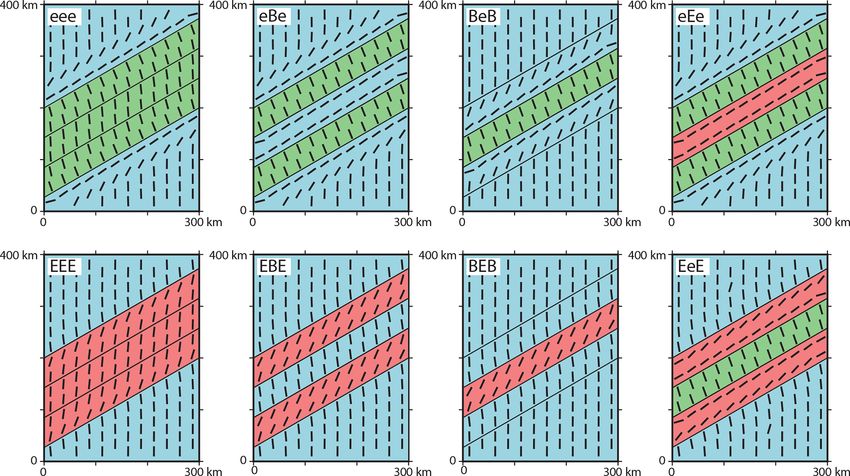
1288 K. Reiter: Stress rotation – impact and interaction of rock stiffness and faults
site: old orogens have apparently no impact on the present- or man-made activities in the underground (e.g. Martínez-
day crustal stress pattern, e.g. the Appalachian Mountains Garzón et al., 2013; Ziegler et al., 2017; Müller et al., 2018).
(Plumb and Cox, 1987; Evans et al., 1989) or Fennoscan- On a map view, several potential sources of stress can su-
dia (Gregersen, 1992). Deviations from the assumed uniform perpose on another and the resulting stress at a certain point
plate-wide stress pattern (here called stress rotations) are ob- comprises the sum of all stress sources from those plate-wide
served recently in several regions, such as in Australia, Ger- to very local stress sources. Differences between the result-
many and North America (Reiter et al., 2015; Heidbach et al., ing stress orientation and the regional stress source can be
2018; Lund Snee and Zoback, 2018, 2020). However, these described by the angular deviation (Sonder, 1990), which can
effects can only be partly explained by the topography or be substantial and can lead to a change of the stress regime
lithospheric structures. (Sonder, 1990; Zoback, 1992; Jaeger et al., 2007). The stress
The complex stress pattern in central–western Europe regime (Anderson, 1905, 1951) is defined by the relative
was a subject of several numerical investigations in recent stress magnitudes, which are a normal faulting regime (SV >
decades (Grünthal and Stromeyer, 1986, 1992, 1994; Gölke SHmax > Shmin ), strike slip regime (SHmax > SV > Shmin ) and
and Coblentz, 1996; Goes et al., 2000; Marotta et al., 2002; thrust faulting regime (SHmax > Shmin > SV ), where SV is the
Kaiser et al., 2005; Jarosiński et al., 2006). Apart from a vertical stress and Shmin and SHmax are the minimum- and
recent 3-D model (Ahlers et al., 2020), the previous mod- the maximum horizontal stress, respectively. The difference
els were limited to 2-D. These 2-D models were able to re- between the largest and smallest principal stress is the dif-
produce some of the observed stress patterns by considering ferential stress (σD = σ1 − σ3 ), while the deviatoric stress is
variable lateral elastic material properties or discontinuities. the difference between the stress state and the mean stress
However, 2-D models have some limitations: they have to (δσ ij = σ ij − σ m ; Engelder, 1994)
integrate topography, crustal thickness and stiffness to one Stress rotation within this study means an angular devia-
property, and they potentially overestimate the horizontal tion of the SHmax orientation from the large-scale stress pat-
stress magnitude (van Wees et al., 2003; Ghosh et al., 2006). tern. In the following subsections, previous observations and
Furthermore, none of these previous studies investigated the models on the respective causes are reviewed and also sum-
impact of the influencing factors separately. marized in Table 1.
In this work, a series of large-scale 3-D generic geome-
chanical models is used to determine which properties can 2.2 Density contrast and topography
cause significant stress rotations at a distance (> 10 km) from
material transitions or discontinuities. The model geometry Variability of density within the crust or lithosphere has a sig-
is inspired by the crustal structure and the stress pattern in nificant impact on the stress state (Frank, 1972; Artyushkov,
the German Central Uplands, where the SHmax orientation is 1973; Fleitout and Froidevaux, 1982; Humphreys and
120 to 160◦ . This is in contrast to a N–S orientation (∼ 0◦ ) of Coblentz, 2007; Ghosh et al., 2009; Naliboff et al., 2012).
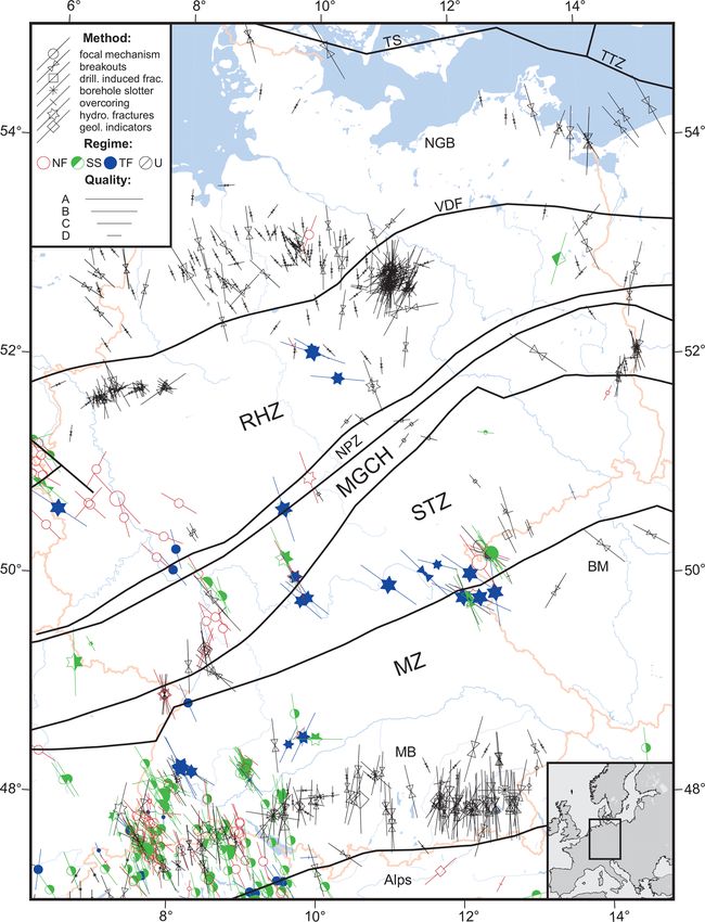
SHmax to the north and to the south of the uplands (Fig. 1, Re- Assameur and Mareschal (1995) showed that local stress in-
iter et al., 2015). The basement structures there are striking creases due to topography and crustal inhomogeneities are in
45 to 60◦ , which is almost perpendicularly to the observed the order of tens of MPa, which is on the order of stresses
SHmax orientation. The influence of the structures on the resulting from the plate boundary forces.
stress field will be tested with a generic variation of Young’s Gravitational forces are also derived by surface topogra-
modulus, Poisson’s ratio, the density and vertical low-friction phy (Zoback, 1992; Miller and Dunne, 1996). Within moun-
discontinuities, which separate the crustal blocks. Each prop- tains, SHmax is oriented parallel to the ridge and perpendic-
erty is tested separately first, to avoid interdependencies; pos- ular to the ridge at the base of the mountain chain. Along
sible interactions are tested afterwards. passive continental margins, effects similar to those due to to-
pography can be observed (Bott and Dean, 1972; Stein et al.,
1989; Bell, 1996; Yassir and Zerwer, 1997; Tingay et al.,
2 Stress rotation in the upper crust 2005; King et al., 2012).
Sonder (1990) investigated the interaction of different re-
2.1 Concept of stress rotation gional deviatoric stress regimes (δσ ij ) with stresses aris-
ing from buoyancy forces (σ G ) and observed a rotation of
This study focuses on stress rotations that occur horizontally, SHmax of up to 90◦ . According to that, SHmax rotates toward
i.e. in the map view. A vertically uniform stress field is as- the normal trend of the density anomaly. If regional stresses
sumed, which is consistent with previous studies (Zoback are large, compared to stresses driven by a density anomaly
et al., 1989; Zoback, 1992; Heidbach et al., 2018). Stress (δσ ij /σ G
1), the influence of a density anomaly is small
rotations with depth are occasionally observed within deep and vice versa: if the regional stress is small compared to the
wells (Zakharova and Goldberg, 2014; Schoenball and Da- stress driven by the density anomaly (δσ ij /σ G
1), the im-
vatzes, 2017), due to evaporites (e.g. Roth and Fleckenstein, pact of a density anomaly on the resulting stress field is large.
2001; Röckel and Lempp, 2003; Cornet and Röckel, 2012) In the case that both stress sources are on a similar level
Solid Earth, 12, 1287–1307, 2021 https://doi.org/10.5194/se-12-1287-2021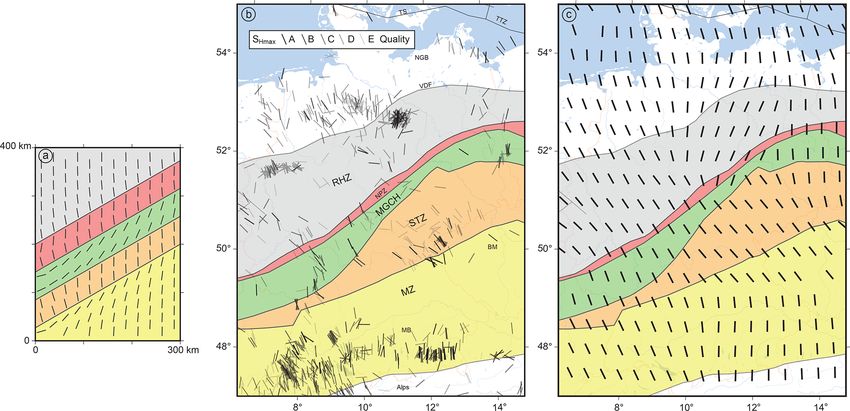
K. Reiter: Stress rotation – impact and interaction of rock stiffness and faults                                                        1289

Table 1. Comparison of selected previous observations or models on the subject of stress rotation in the context of faults, elastic material
properties, density or topography variation. The characters “X” and “V” indicate whether the property is included or varied; “(X)” means
that the subject is included indirectly. The characters “ < ” and “ > ” indicate that significant rotation occurs near (< 10 km) or at greater
distance (> 10 km) from the fault or material transition.

  Publication                       Model (M) or       Density/     Max. observed     Young’s     Poisson’s   Faults   Significant rotation
                                    observation (O)    thickness      rotation [◦ ]   modulus     ratio                > or < 10 km
  Grünthal and Stromeyer (1986)     M                  –                         90   X           X           –        >
  Bell and Lloyd (1989)             M                  –                       ∼ 25   V           V           –        >
  Bell and McCallum (1990)          O                  –                         90   –           –           X        <
  Sonder (1990)                     M                  V                         90   –           –           –        –
  Grünthal and Stromeyer (1992)     M                  –                         90   V           X           X        >
  Grünthal and Stromeyer (1994)     M                  –                         90   V           X           X        >
  Spann et al. (1994)               M                  –                         90   V           X           –        >
  Zhang et al. (1994)               M                  –                         58   V           V           –        >
  Gölke and Coblentz (1996)         M                  X                       ∼ 45   X           X           –        >
  Homberg et al. (1997)             M                  X                         50   X           X           X        <
  Mantovani et al. (2000)           M                  (X)                       90   V           X           V        >
  Marotta et al. (2002)             M                  X                       ∼ 35   –           –           –        >
  Yale (2003)                       O                  –                         90   –           –           X        <
  Jarosiński et al. (2006)         M                  (X)                       90   V           X           V        >
  Mazzotti and Townend (2010)       O                  –                         50   –           –           X        >

(δσ ij /σ G ≈ 1), small changes of one of the stress sources             stresses must be oriented perpendicular to the frictionless
are able to change the stress regime, and thus potentially the           fault; the two remaining ones are parallel to the discontinu-
stress orientation.                                                      ity. For this reason, the stress tensor rotates near a frictionless
                                                                         fault, depending on its orientation. Significant stress rotation
2.3   Stiffness contrast                                                 in the context of faults is reported (Bell and McCallum, 1990;
                                                                         Adams and Bell, 1991; Yale, 2003; Mazzotti and Townend,
Mechanical stiffness describes the material behaviour under              2010). However, Yale (2003) assumes that stress rotation oc-
the influence of stress and strain. The focus here is on linear          curs only within several kilometres from the fault. Large dif-
elastic material properties, characterized by Young’s modu-              ferential stress leads to a more stable stress pattern (Laubach
lus and Poisson’s ratio. Stress refraction between two elastic           et al., 1992; Yale, 2003), whereas low differential stresses al-
media can be calculated, but only at the interface of the two            low a switch of the stress regime caused by faults. The impact
media, based on the known stress state on one side of the                of faults on stress rotation has been investigated analytically
interface and Young’s modulus on both sides (Spann et al.,               (Saucier et al., 1992) and by numerical models (e.g. Zhang
1994). Stress rotation due to stiffness contrast is for exam-            et al., 1994; Tommasi et al., 1995; Homberg et al., 1997).
ple reported for the Peace River Arch in Alberta, Canada
(Fordjor et al., 1983; Bell and Lloyd, 1989; Adams and Bell,
1991). Potential stress rotation is supported by several nu-             3     Regional setting
merical studies (e.g. Bell and Lloyd, 1989; Grünthal and
Stromeyer, 1992; Spann et al., 1994; Zhang et al., 1994;                 3.1    Stress orientation in central Europe
Tommasi et al., 1995; Mantovani et al., 2000; Marotta et al.,
2002).                                                                   Crustal stress data from Europe have been collected since the
                                                                         1960s (e.g. Hast, 1969, 1973, 1974; Greiner, 1975; Ranalli
2.4   Discontinuities                                                    and Chandler, 1975; Greiner and Illies, 1977; Froidevaux
                                                                         et al., 1980; Kohlbeck et al., 1980), later as part of the World
Discontinuities are planar structures within or between rock             Stress Map database from Zoback et al. (1989) and more re-
units, where the shear strength is (significantly) lower than            cently by Heidbach et al. (2018).
that of the surrounding rock. Genetically, discontinuities can              SHmax orientation in western Europe is 145◦ ± 26◦ and
be classified into bedding, schistosity, joints and fault planes.        rotates clockwise by about 17◦ (Müller et al., 1992) to the
In the context of this study the term discontinuity refers               direction of absolute plate motion from Minster and Jordan
to fault planes or fault zones. Similar to the Earth surface,            (1978). This is in agreement with Zoback et al. (1989), who
(nearly) frictionless faults without cohesion act like a free            obtained a better fit for relative plate motion between Africa
surface in terms of continuum mechanics (Bell et al., 1992;              and Europe than for absolute plate motion. As the major
Bell, 1996; Jaeger et al., 2007). One of the three principal             causes of the observed stress pattern in western and central

https://doi.org/10.5194/se-12-1287-2021                                                               Solid Earth, 12, 1287–1307, 2021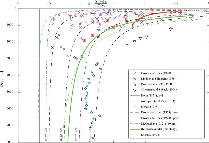
1290                                          K. Reiter: Stress rotation – impact and interaction of rock stiffness and faults

Europe, the ridge push of the Mid-Atlantic ridge and the col-       3.2   Basement structures in Germany
lisional forces along the southern plate margins are identi-
fied (Richardson et al., 1979; Grünthal and Stromeyer, 1986;        In large part, Germany consists of Variscan basement units,
Klein and Barr, 1986; Zoback et al., 1989; Grünthal and             either exposed or covered by Post-Paleozoic basin sediments.
Stromeyer, 1992; Müller et al., 1992; Zoback, 1992; Gölke           The Variscan orogen is a product of the late-Paleozoic colli-
and Coblentz, 1996; Goes et al., 2000).                             sion of the plates Gondwana and Avalonia (Laurussia) in late
   A fan-like stress pattern has been observed in the western       Devonian to early Carboniferous time, which lead to closure
Alps and Jura mountains, where SHmax in front of the moun-          of the Rheic Ocean (Matte, 1986), and finally the formation
tain chain is perpendicular to the strike of the orogen (Fig. 1).   of the super-continent Pangaea. Despite the fact that the Eu-
Müller et al. (1992) assume that these structures only locally      ropean Variscides are well investigated in the last century and
overprint the general stress pattern. However, in light of the      decades (e.g. Franke, 2000, 2006; Kroner et al., 2007; Kroner
recently available data, it is assumed that the SHmax orienta-      and Romer, 2013), it is for example still a matter of debate
tion is rather controlled by gravitational potential energy of      whether several microplates have been amalgamated in be-
the alpine topography than by plate boundary forces (Grün-          tween or not.
thal and Stromeyer, 1992; Reinecker et al., 2010).                     Kossmat (1927) published the structural zonation of the
   The stress pattern in western and central Europe has been        European Variscides, which is still widely used (Fig. 1).
the subject of several modelling attempts in the last three         The parts to the north-west of the Rheic Suture Zone are
decades (Grünthal and Stromeyer, 1986, 1992, 1994; Gölke            the Rheno-Hercynian Zone (RHZ) with the sub-unit of the
and Coblentz, 1996; Goes et al., 2000; Marotta et al., 2002;        Northern Phylite Zone (NPZ), both of Laurussian origin.
Kaiser et al., 2005; Jarosiński et al., 2006). In particu-         South-east of the suture zone are the Mid-German Crystalline
lar, these previous studies investigated the impact of a lat-       High (MGCH), the Saxo-Thuringian Zone (STZ) and the
eral stiffness contrast in the crust (Grünthal and Stromeyer,       Moldanubian Zone (MZ); all except the MGCH were exclu-
1986, 1992, 1994; Jarosiński et al., 2006; Kaiser et al., 2005;    sively part of Gondwana.
Marotta et al., 2002), the elastic thickness of the lithosphere        The RHZ is exposed in the Rhenish Massif, in the
(Jarosiński et al., 2006), the stiffness contrast of the mantle    Harz mountains and in the Flechtingen Hills. Dominant are
(Goes et al., 2000), a lateral density contrast or topographic      Devonian to lower Carboniferous clastic shelf sediments
effects (Gölke and Coblentz, 1996; Jarosiński et al., 2006),       (Franke, 2000; Franke and Dulce, 2017). These low meta-
the post-glacial rebound in Scandinavia (Kaiser et al., 2005),      morphic slates, sandstones, greywacke and quartzite are sup-
and activity on faults (Kaiser et al., 2005; Jarosiński et al.,    plemented with continental and oceanic volcanic rocks, reef
2006).                                                              limestones and a few older gneisses. Further to the north of
   Stiffness variation in the lithosphere, e.g. in the Teisseyre–   the RHZ are the sub-Variscan foreland deposits, consisting
Tornquist Zone (TTZ) or the Bohemian Massif (BM),                   of clastic sediments and coal seams.
has been identified as a potential cause for the observed              The NPZ is uncovered at the southern edge of the low
stress rotation in Central Europe (Grünthal and Stromeyer,          mountain ranges Hunsrück, Taunus and eastern Harz. Petro-
1986, 1992, 1994; Gölke and Coblentz, 1996; Reinecker               logically it is probably the greenschist facies equivalent
and Lenhardt, 1999; Goes et al., 2000; Marotta et al., 2002;        (Oncken et al., 1995) of the Rheno-Hercynian shelf se-
Kaiser et al., 2005). One example is the fan-shaped stress          quence (Klügel et al., 1994), consisting of meta-sediments
pattern in the North German Basin (NGB), with a rotation            and within-plate metavolcanic rocks (Franke, 2000).
of SHmax from north-west in the western part to north-east in          The MGCH is open in the Palatinate Forest, Odenwald,
the eastern part of the basin as a product of the TTZ, which        Spessart, Kyffhäuser, Ruhla Crystalline (Thuringian Forest)
is the boundary between the Phanerozoic Europe (Avalonia)           and Flechtingen Hills. It has been interpreted previously as
and the much stiffer Precambrian Eastern European Craton            a magmatic arc of the Saxo-Thuringian Zone. But Oncken
(Baltica).                                                          (1997) assumes that the MGCH is composed of both Saxo-
   Jarosiński et al. (2006) came to the conclusion that active     Thuringian and Rheno-Hercynian rocks. Composition and
tectonic zones and topography have major effects, whereas           metamorphic grade vary considerably along the strike of the
the stiffness contrast leads only to minor effects. Lateral vari-   MGCH (Franke, 2000). It consists of late-Paleozoic sedi-
ation of density does not have a significant impact on the          ments, meta-sediments, volcanic rocks, granitoides, gabbros,
stress pattern (Gölke and Coblentz, 1996); it causes only           amphibolite and gneisses.
local effects. Finally, low differential stress allows signifi-        The Saxo-Thuringian Zone (STZ) is exposed in the
cant stress rotation (Sonder, 1990; Grünthal and Stromeyer,         Thuringian-Vogtlandian Slate Mountains, Fichtel Moun-
1992).                                                              tains, Ore Mountains, Saxonian Granulite Massif, Elbe Val-
                                                                    ley Slate Mountains and the Lausitz. It consists of Campro-
                                                                    Ordovician mafic and felsic magmatic rocks and late Ordovi-
                                                                    cian to early Carboniferous marine and terrestrial sediments
                                                                    (Franke, 2000; Linnemann, 2004). These rocks underwent

Solid Earth, 12, 1287–1307, 2021                                                       https://doi.org/10.5194/se-12-1287-2021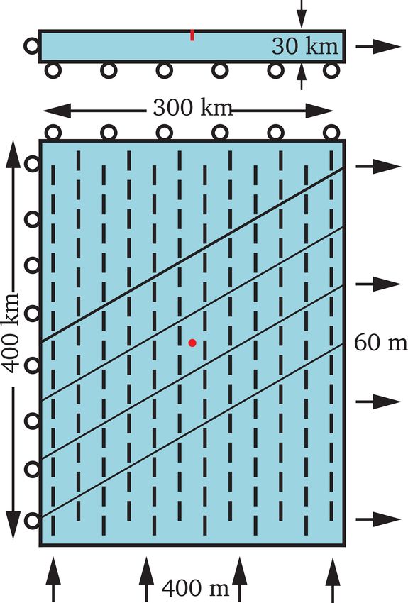
K. Reiter: Stress rotation – impact and interaction of rock stiffness and faults                                                    1291

                                                                   Figure 2. Reference model with the applied boundary conditions,
                                                                   used for all models, in map view and from the south. The model
                                                                   has a lateral extent of 300 km × 400 km and a thickness of 30 km.
                                                                   It consists of five interconnected units, which have the same mate-
                                                                   rial properties. Blue visualizes the reference material (Table 2). The
                                                                   boundary conditions ban motion in the x direction on the western
                                                                   side, in the y direction on the northern side and in the z direction at
                                                                   the model base. A push of 400 m from the south and a pull of 60 m
                                                                   to the east is applied. The resulting SHmax orientation (north–south)
                                                                   at a depth of 1000 m is illustrated by the black bars. The red point
                                                                   (and line) indicates the location of the virtual well (Figs. 4 and 5).
                                                                   The four diagonal boundaries can be used as vertical faults with a
                                                                   chosen friction coefficient.
Figure 1. Stress orientation in the German Central Uplands with
the basement structural elements (separated by black lines), po-
litical boundaries (red) and major rivers (blue). Bars represent   4     Model set-up
orientation of maximum horizontal compressional stress (SHmax );
line length is proportional to quality. Colours indicate stress    4.1    Model geometry
regimes, with red for normal faulting (NF), green for strike–
slip faulting (SS), blue for thrust faulting (TF) and black for    The chosen model geometry is inspired by the geometrical
unknown regime (U). The Variscan basement structures intro-        situation in the German Central Uplands (Fig. 1), but the
duced by Kossmat (1927) are visualized; the regional segmenta-     overall intention is a generic model. To make it easy to un-
tion is as follows: BM = Bohemian Massif, MGCH = Mid-German        derstand, compass directions are used for the model descrip-
Crystalline High, MZ = Moldanubian Zone, NPZ = Northern Pyl-
                                                                   tion. The model geometry has a north–south extent of 400
lite Zone, RHZ = Rheno-Hercynian Zone, STZ = Saxo-Thuringian
Zone, and VDF = Variscan Deformation Front. Other structures are
                                                                   and 300 km in the east–west direction, with a thickness of
as follows: MB = Molasses Basin; NGB = North German Basin,         30 km (Fig. 2). In the centre of the model, three diagonal
TS = Thor Suture, TTZ = Teisseyre–Tornquist Zone (redrawn after    units each with a width of 50 km are oriented 60◦ from the
Franke, 2014; Grad et al., 2016).                                  north. The unit boundaries are vertically incident. A model
                                                                   variant is generated in which the unit boundaries allow free
                                                                   sliding, depending on a chosen friction coefficient. For each
metamorphic overprint up to the early Carboniferous with           of the three central units, different material properties can be
different metamorphism stages up to eclogite- or granulite         applied. The northernmost and southernmost block has al-
facies. These units are interspersed by late- or post-orogenic     ways the same (reference) material properties, except for the
granites.                                                          realistic rock property scenario.
   The MZ is exposed in the Bohemian Massif, the Bavar-
ian Forest, the Münchberg Gneiss Massif, the Black Forest          4.2    Solution of the equilibrium of forces
and the Vosges. They consist of mostly high-grade metamor-
phic crystalline rocks (gneisses, granulite, migmatite) and        The stress orientations in the models are investigated using
Variscan granites (Franke, 2000).                                  the finite-element method (FEM). The usage of 3-D FEM
                                                                   models to investigate the stress state in the crust is a well-
                                                                   established technique (e.g. van Wees et al., 2003; Buchmann
                                                                   and Connolly, 2007; Hergert and Heidbach, 2011; Reiter and

https://doi.org/10.5194/se-12-1287-2021                                                          Solid Earth, 12, 1287–1307, 2021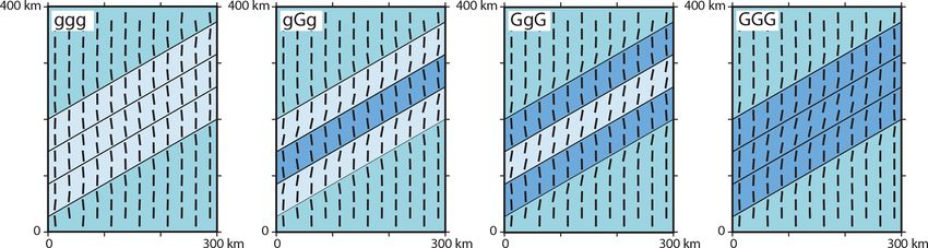
1292                                           K. Reiter: Stress rotation – impact and interaction of rock stiffness and faults

Figure 3. Selection of common elastic rock properties (Young’s modulus and Poisson’s ratio) and density (Turcotte et al., 2014). Coloured
vertical bars indicate applied material properties; see Table 2.

Heidbach, 2014; Hergert et al., 2015). The major reason that           Table 2. Young’s modulus, Poisson’s ratio and densities used in
complex 2-D or 3-D models can be computed is the opportu-              the models. Bold numbers indicate the properties used, which differ
nity to use unstructured meshes.                                       from those of the reference material.
   The method in general computes the equilibrium of
stresses arising from boundary forces (via displacement                                             Young’s     Poisson’s
                                                                          Name                      modulus          ratio    Density
boundary conditions) and body forces (gravity) acting on the
                                                                                                      [GPa]            [–]   [g cm−3 ]
rock whose mechanical behaviour is characterized by a con-
stitutive law and associated material parameters. The equilib-            Reference material (B)          50         0.25          2.7
rium of forces is represented by partial differential equations,          Low density (g)                 50         0.25          2.2
which are solved numerically.                                             High density (G)                50         0.25          3.2
                                                                          Low Poisson (p)                 50         0.15          2.7
δσ ij                                                                     High Poisson (P)                50         0.35          2.7
      + ρxi = 0,                                              (1)         Low stiffness (e)               10         0.25          2.7
δxj
                                                                          High stiffness (E)             100         0.25          2.7
where δσ ij is the variation of total stress, δxj is the spatial          Upper mantle                   130         0.25         3.25
change and ρxj represents the weight of the rock section
(ρ = density). Linear elastic material behaviour expressed by
Hooke’s law is assumed. Two material properties, Young’s
modulus (E) and Poisson’s ratio (ν) are essential. The stress          modulus (E) and Poisson’s ratio (ν) of representative rocks,
state in this study will be calculated based on defined dis-           taken from a textbook (Turcotte et al., 2014).
placement boundary conditions (Fig. 2).                                   The reference material for this investigation has a den-
   The lateral resolution of the model is about 3 km, con-             sity of ρ = 2.7 g cm−3 , a Poisson’s ratio of ν = 0.25 and
sisting primarily of hexahedrons and some wedge elements               a Young’s modulus of E = 50 GPa. Such a material could
(degenerated hexahedrons). Resolution into depth ranges                represent for example granite or limestone. Based on this
from 0.44 km near the surface to about 3.4 km at the base              reference material, a lower and higher material value is al-
of the model. In total, about 166 000 elements were used.              ways defined (Table 2), which is within the range of com-
The model version with contact surfaces uses 1725 con-                 mon rock properties (Fig. 3). The material with a low density
tact elements along each contact surface. Model discretiza-            (ρ = 2.2 g cm−3 ) may represent sediments (sandstone, lime-
tion was performed with HyperMesh® v.2019. The equi-                   stone, shale etc.), whereas the high-density material (ρ =
librium of forces (body forces and boundary condition) is              3.2 g cm−3 ) could represent a rock from the lower crust or
computed numerically using the Abaqus® /Standard v.6.14-1              the upper mantle. A low Poisson’s ratio (ν = 0.15) may rep-
finite-element software.                                               resent sediments (sandstone or shale), and a high Poisson’s
                                                                       ratio (ν = 0.35) could represent ultramafic rocks. Soft mate-
4.3    Mechanical properties                                           rial with a low Young’s modulus (E = 10 GPa) may repre-
                                                                       sent sediments, pre-damaged rock or weathered rock. Again
The main subject of this study is to investigate the impact            ultramafic rock is an example of a stiff rock, having a large
of the variation of elastic rock properties, density and fric-         Young’s modulus (E = 100 GPa).
tion along faults on stress orientation in the upper crust in             Laboratory rock experiments in the past delivered friction
the given geometrical setting outlined in the previous sec-            coefficients of about µ = 0.6 to 0.85 (Byerlee, 1978). How-
tions (Fig. 2). To do this, each parameter is tested individ-          ever, recent investigations using realistic slip rates for earth-
ually. Figure 3 visualizes the range of density (ρ), Young’s           quakes decreased estimated friction coefficients by 1 order of

Solid Earth, 12, 1287–1307, 2021                                                           https://doi.org/10.5194/se-12-1287-2021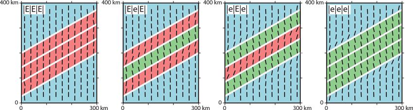
K. Reiter: Stress rotation – impact and interaction of rock stiffness and faults                                                            1293

Figure 4. The stress ratio k (Eq. 3) is plotted vs. depth. Stress in the reference model is marked with the bold green line. Additionally, several
data and defined stress ratios from the literature are visualized for comparison (Heim, 1878; Herget, 1973; Brown and Hoek, 1978; Lindner
and Halpern, 1978; McCutchen, 1982; Sheorey, 1994; Brudy et al., 1997; Hickman and Zoback, 2004).

magnitude down to µ < 0.1 (Di Toro et al., 2011). Faults are               large friction coefficient (µ = 10) to prevent slip. At a virtual
represented by cohesionless contact surfaces in the models.                well in the centre of the model (x = 150 km; y = 200 km)
The used friction coefficients are 0.1, 0.2, 0.4, 0.6, 0.8 and             stress was extracted from the model and compared to the
1.0, which covers both slow and fast slip rates.                           stress magnitude data, which are visualized in Figs. 4 and
                                                                           5, showing a good fit to stress–depth distribution assump-
4.4   Initial stress state                                                 tions (Heim, 1878; Herget, 1973; Brown and Hoek, 1978;
                                                                           McCutchen, 1982; Sheorey, 1994) and measured magnitude
The present-day stress state in the crust is a complex product             ratios also (Brown and Hoek, 1978; Lindner and Halpern,
of several stress sources from the past to the present. In or-             1978; Brudy et al., 1997; Hickman and Zoback, 2004).
der to model the stress state an initial stress state is defined,
which is in equilibrium with the body forces (gravity) and                 4.5    Boundary conditions
which subsequently undergoes lateral straining to account
for tectonic stress. Sheorey (1994) provided a simple semi-                The overall SHmax orientation on a virtual profile along lon-
empirical function (Eq. 2) for the stress ratio k (Eq. 3), where           gitude 11◦ (Fig. 1) displays a north–south orientation in the
E is Young’s modulus and z is the depth in kilometres.                     North German Basin (NGB) and in the Molasse Basin (MB)

                          1
                                                                          north of the Alps, except the Variscan basement units in be-
k = 0.25 + 7E 0.001 +                                         (2)          tween. Correspondingly, a north–south orientation of SHmax
                          z
                                                                           is intended for the reference model. In order to generate a
     SHmean     SHmax + Shmin
k=           =                                                (3)          meaningful stress state in the model, appropriate boundary
       SV             2SV                                                  conditions are required, which are technically applied by a
   Sheorey’s equation (Eq. 2) is a reliable stress ratio vs.               defined lateral displacement. Results from a virtual well in
depth estimation, when compared to real-world data (Fig. 4).               the model centre are compared with data from deep wells. An
The model is pre-stressed with zero horizontal strain bound-               extension of 60 m (x = 2 × 10⁻⁴ ) in the east–west direction
ary conditions. The pre-stressing method used here has so                  and a shortening of 400 m (y = −1 × 10⁻³ ) in the north–
far been used several times (Buchmann and Connolly, 2007;                  south direction (Fig. 2) provide a good fit of the reference
Hergert and Heidbach, 2011; Reiter and Heidbach, 2014).                    model to stress magnitudes from selected deep wells (Fig. 5,
The model is allowed to compact several times under ap-                    Brudy et al., 1997; Hickman and Zoback, 2004; Lund and
plication of the body forces (gravity) using a Poisson’s ra-               Zoback, 1999). By fitting the data, the focus was more on
tio of ν = 0.396 during that procedure only. During the pre-               the observed Shmin magnitudes and to a lesser extent on the
stressing procedure, models with contact surfaces have a very              SHmax magnitudes. The latter are less reliable, as they are

https://doi.org/10.5194/se-12-1287-2021                                                                  Solid Earth, 12, 1287–1307, 2021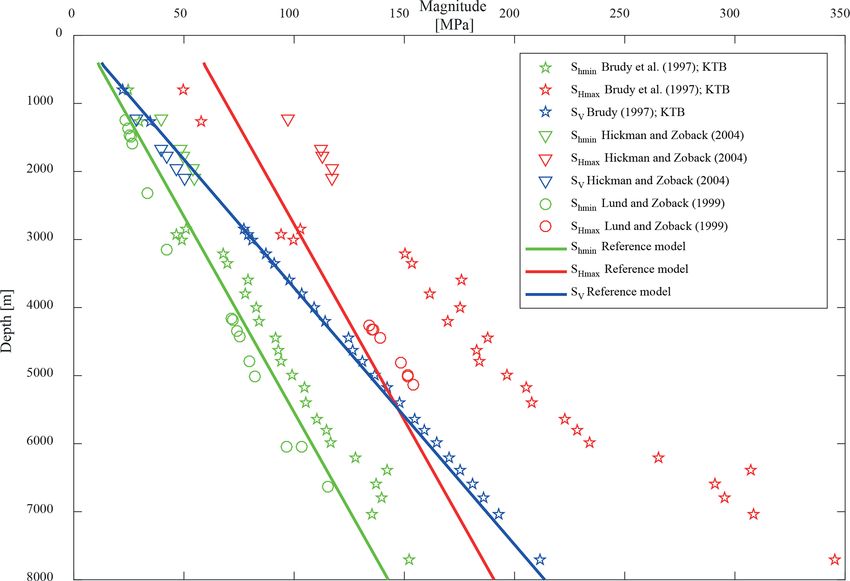
1294                                            K. Reiter: Stress rotation – impact and interaction of rock stiffness and faults

Table 3. Material properties used for the scenario using realis-      sediments, and some volcanites. Therefore, this zone is a
tic rock properties for Variscan basement units; properties are es-   stiff unit. The Saxo-Thuringian Zone (STZ) is dominated
timated based on Turcotte et al. (2014). MGCH = Mid-German            by meta-sediments, mafic and felsic magmatites and their
Crystalline High, MZ = Moldanubian Zone, NPZ = Northern Pyl-          metamorphosed equivalents, and some high-grade metamor-
lite Zone, RHZ = Rheno-Hercynian Zone, STZ = Saxo-Thuringian          phic rocks (granulite, eklogite). Taking all the different rock
Zone.
                                                                      types into account, the STZ is stiffer than the RHZ and
                                  Young’s     Poisson’s
                                                                      softer than the MGCH. Mechanically, the MZ can be repre-
          Variscan     Density    modulus          ratio              sented by high-grade metamorphic rocks (gneiss, granulite,
          units              ρ         E               ν              migmatite) and granitoids and will be a stiff unit, similar to
                      [g cm−3 ]    [MPa]              []              the MGCH. Therefore, the unit stiffnesses are different: they
                                                                      are from slightly deformable to rigid in the following or-
          RHZ              2.10          20        0.15               der: RHZ ≈ NPZ < STZ < MGCH ≈ MZ. Material proper-
          NPZ              2.20          30        0.15
                                                                      ties used are estimated based on typical rock values (Table 3).
          MGCH             2.75          70        0.30
          STZ              2.60          50        0.25
                                                                      The same initial stress procedure, boundary condition and vi-
          MZ               2.75          70        0.30               sualization procedure are applied as previously described.

                                                                      5     Results
usually not measured; they are calculated on the basis of sev-
eral assumptions. The determined boundary conditions are              5.1    Density influence
used for all models.
                                                                      To identify the influence of a density variation, the refer-
4.6    Generic model scenario’s                                       ence density (ρ = 2.7 g cm−3 ) in blue is varied using a small
                                                                      density (g: ρ = 2.2 g cm−3 ), which is coloured in light blue,
The model geometry consists of five units (Fig. 2). The               and a large density (G: ρ = 3.2 g cm−3 ), which is dark blue
northern- and southernmost blocks are always assigned the             (Fig. 6).
reference material properties (Table 2). In between there are            The low-density anomaly (ggg) results in a slight counter-
three diagonal units in which material properties are varied.         clockwise (−6◦ ) rotation of the SHmax orientation in the ref-
Along the vertical borders within the model, friction proper-         erence material near the anomaly (Fig. 6). Within the low-
ties can be used. The lower (L) or higher (H) values of the           density units near the reference material, nearly no rota-
material properties with respect to the reference material (B)        tion is observed (−1◦ ), but SHmax orientation turns counter-
will be varied in the following way: LLL, HHH, LBL, BLB,              clockwise (−8◦ ) in the centre of the material anomaly. The
etc. When the model geometry mimics discontinuities using             angular variation of SHmax crossing the units is of the order
contact surfaces, all contacts have the same friction coeffi-         of 7◦ . The high-density anomaly (GGG) results in a slightly
cient. In the figures showing the results the label “|” indicates     clockwise rotation (+7◦ ) in the reference material near the
contact. For example, HLH with four contacts is |H|L|H|.              anomaly. In the high-density unit near the reference mate-
   The SHmax orientation is visualized at a depth of 1000 m           rial, SHmax is minimally influenced (+1◦ ) but rotates further
below the surface using a pre-defined grid, where the lat-            clockwise (+12◦ ) in the centre of the anomaly. Based on that,
eral distance to the material transition or discontinuity is          the variation across the units is about 11◦ . The models with
> 12.5 km, as far-field effects are the main interest of this         mixed densities in the three units show a clockwise rotation
study. The variation of density, Poisson’s ratio, Young’s mod-        (+10◦ ) of SHmax within the lighter material next to the denser
ulus and friction coefficient will be tested first. In addition,      units. The high-density units show a counter-clockwise rota-
the variation of Young’s modulus is tested in interaction with        tion (−7◦ ) next to the low-density unit; therefore, the total
low-friction contacts.                                                variation of SHmax is 17◦ .
                                                                         In general, SHmax tends to be oriented parallel to the
4.7    Realistic rock property scenario                               anomaly in low-density units and perpendicular to the
                                                                      anomaly in large density units. In the centre of the low-
A reality-based rock property scenario, inspired by the struc-        density units (ggg), the stress orientation becomes perpendic-
tural zonation of the European Variscides according to Koss-          ular to the overall structure. In the centre of the high-density
mat (1927), is tested. The RHZ and the NPZ are dominated              units (GGG) the opposite is true, and SHmax becomes parallel
by clastic shelf sediments with a low- or mid-metamorphic             to the structure.
overprint, which is made of slate (RHZ) and phyllite (NPZ).
This zone, the RHZ and the NPZ together, is the most flex-            5.2    Influence of Poisson’s ratio
ible one and will have the lowest Young’s modulus (Ta-
ble 3). The MGCH consists of granitoids or gabbros and                The influence of Poisson’s ratio on the stress rotation is tested
their metamorphic equivalents (gneiss, amphibolite), meta-            by variation of the reference Poisson’s ratio (ν = 0.25) us-

Solid Earth, 12, 1287–1307, 2021                                                          https://doi.org/10.5194/se-12-1287-2021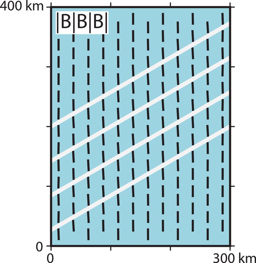
K. Reiter: Stress rotation – impact and interaction of rock stiffness and faults                                                         1295

Figure 5. The stress magnitudes are plotted as a function of depth. The stress components from the virtual well in the model are illustrated
by the coloured lines. The location of the virtual well and boundary conditions used are shown in Fig. 2. Due to the applied initial stress
conditions, the stress regime changes from thrust faulting at a depth of 400 m to strike slip faulting, and finally to a normal faulting regime
at a depth greater than 5500 m. Published stress magnitude data are shown for comparison (Brudy et al., 1997; Lund and Zoback, 1999;
Hickman and Zoback, 2004).

Figure 6. Influence of density on the stress orientation. Black bars represent the orientation of SHmax at a depth of 1000 m. Colours indicate
the material properties used. The medium blue area uses the reference material properties (ρ = 2.7 g cm−3 ), the light blue material uses a
lower density (g: ρ = 2.2 g cm−3 ), the dark blue a larger density (G: ρ = 3.2 g cm−3 ).

ing a lower one (p: ν = 0.15) in light purple and a larger                5.3   Impact of Young’s modulus
one (P: ν = 0.35) in dark purple (Fig. 7). The models with
only a lower (ppp: −1.5◦ ) and only a higher Poisson’s ra-                The impact of Young’s modulus is investigated using the ref-
tio (PPP: +2.2◦ ) show only little SHmax rotation (Fig. 7).               erence material (B: E = 50 GPa) in contrast to a softer mate-
Mixed models with largest Poisson’s ratio variation (pPp and              rial (e: E = 10 GPa) in green and a stiffer material (E: E =
PpP) have some counter-clockwise rotation in the low Pois-                100 GPa) in red (Fig. 8). The models with the soft units
son’s ratio units (−3.0◦ ) and a clockwise rotation in the high           (eee, eBe and BeB) exhibit a strong clockwise SHmax rotation
Poisson’s ratio units (+4.2◦ ). Therefore, the total variance of          (+56◦ ) in the units with the reference material and a counter-
SHmax is about 7.5◦ .                                                     clockwise rotation in the softer units (−22◦ ) near the mate-
                                                                          rial transitions. For the models with three soft units (eee) the
                                                                          SHmax orientation decreases to −5◦ in the centre of the units.
                                                                          This means that the SHmax variation within the soft units is

https://doi.org/10.5194/se-12-1287-2021                                                                Solid Earth, 12, 1287–1307, 2021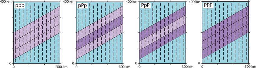
1296                                              K. Reiter: Stress rotation – impact and interaction of rock stiffness and faults

Figure 7. Influence of Poisson’s ratio on the stress orientation. Black bars represent the orientation of SHmax at a depth of 1000 m. Colours
indicate the material properties used. The blue area uses the reference material properties (ν = 0.25), the light purple area is characterized by
a low Poisson’s ratio (p: ν = 0.15) and the dark purple one by a large Poisson’s ratio (P: ν = 0.35).

Figure 8. Influence of Young’s modulus variation on the stress orientation. Black bars represent the orientation of SHmax at a depth of
1000 m. Colours indicate the used Young’s modulus; the blue area uses the reference material properties (B: E = 50 GPa), the green material
uses a low Young’s modulus (e: E = 10 GPa) and the red material has a large Young’s modulus (E: E = 100 GPa).

considerable (17◦ ). The resulting total variation is 78◦ . The            SHmax rotation (−19 to −22◦ ), whereas the stiff units dis-
models with the stiff units (EEE, EBE and BEB) exhibit a                   play a clockwise rotation (+53 to +56◦ ). Consequently, the
gentle counter-clockwise rotation in the units with the refer-             total variation between the soft and stiff units is 72 to 78◦ .
ence material (−5.5 to −7◦ ) next to the stiff units. Within the           The general observation is that next to the material transition,
stiff units, a significant clockwise rotation (+20 to +25◦ ) is            SHmax rotates perpendicular to the anomaly for the compliant
apparent next to the reference units. In the model with three              units and parallel for the stiff units.
stiff units (EEE), the SHmax orientation decreases to (+5◦ )
in the centre. This is a considerable SHmax variation of 15◦               5.4   Influence of faults
within the stiff units. The total variation is 31◦ .
   For the models with alternating soft and stiff material units           Several models with the reference material properties sepa-
(EeE and eEe), the soft units exhibit a counter-clockwise                  rated by three discontinuities (|B|B|B|) with a friction coef-

Solid Earth, 12, 1287–1307, 2021                                                                https://doi.org/10.5194/se-12-1287-2021
K. Reiter: Stress rotation – impact and interaction of rock stiffness and faults                                                       1297

                                                                           5.6    Stress rotation for realistic material properties

                                                                           The resulting SHmax orientation (Fig. 11a) of the model us-
                                                                           ing realistic material properties (Table 3) indicates counter-
                                                                           clockwise rotation in the RHZ and NPZ and clockwise ro-
                                                                           tation within the MGCH and MZ units. The overall pattern
                                                                           of the simple model (Fig. 11a) shows only limited similarity
                                                                           with the observed and the mean SHmax orientation on a reg-
                                                                           ular grid using a search radius of 150 km and a quality and
                                                                           distance weight (Fig. 11b and c). However, some similarities
                                                                           can be observed. For example, the simple model (Fig. 11a)
                                                                           shows a clockwise rotation from the NPZ to the MGCH
Figure 9. Influence of low-friction faults on the far-field stress ori-    and counter-clockwise from the MGCH to the STZ. In Fig-
entation. Black bars represent the orientation of SHmax at a depth         ure 11b these areas show similar, but less pronounced, rota-
of 1000 m. All areas have the properties of the reference material         tion of SHmax . The north-north-east SHmax orientation within
(Table 2). White lines indicate cohesionless discontinuities (verti-
                                                                           the central part of the MGCH is similar between the model,
cal faults). The model using a friction coefficient of µ = 0.1 along
                                                                           the data and the mean SHmax orientation (Fig. 11a–c).
the three discontinuities is shown. The other models with a larger
friction coefficient (up to 1 and larger) have similar results; they are
waived out because of the visual similarity.

                                                                           6     Discussion

ficient (µ) from 0.1 to 1 are tested. The low-friction coeffi-             6.1    Model simplification
cient (µ = 0.1) leads to a counter-clockwise SHmax rotation
of only −3◦ (Fig. 9). The maximum observed fault offset is                 This study investigates the influence of elastic material prop-
about 16 m. By increasing the friction coefficient to µ = 0.2,             erties, density and friction coefficient at vertical faults on the
the SHmax rotation is −2◦ ; for µ = 0.4, SHmax rotation is only            orientation of SHmax . The focus is not on stress rotation close
−1◦ . For larger friction coefficients, the SHmax rotation is be-          to the material transition or discontinuity (< 10 km), the pri-
low −1◦ . As the SHmax rotation is too small for a visual dif-             ority is on the far-field effects (> 10 km). Although the model
ferentiation, only the µ = 0.1 model is shown in Fig. 9.                   is inspired by a particular region, the goal is to gain a better
                                                                           understanding on how the variable material properties affect
5.5   Stiffness variation combined with low-friction                       the stress orientation. For this reason, the model geometry is
      faults                                                               very simple and some of the material properties used may
                                                                           have no proper natural equivalent.
The interaction between a significant Young’s modulus con-                    Chosen properties are constant over a depth of 30 km,
trast and a cohesionless contact with a low-friction coeffi-               which is unlikely. Even for a given lithology, the properties
cient (µ = 0.1) is tested along all four discontinuities. The              can change with depth, as a result of the acting gravity and
model with three stiff units (|E|E|E|) provides only little                compaction, especially for sediments. Each lithological unit
counter-clockwise rotation (−4◦ ) in the reference material                is at least partially affected by these changes. Linearly in-
near the material transition (Fig. 10). Similar clockwise ro-              creasing rock properties with depth would account for this
tation occurs in the stiff units (+4◦ ) near the material transi-          and be a more realistic representation. But this would not af-
tion and decreases to the centre of the units (+1◦ ). The total            fect the resulting stress pattern, especially since a vertically
SHmax variation is about 8◦ .                                              uniform stress field is assumed (Zoback et al., 1989; Zoback,
   The model with the soft units and the low-friction discon-              1992; Heidbach et al., 2018), with a few exceptions.
tinuities (|e|e|e|) shows larger rotations than the model with                The simple generic models neglect various rheological
stiffer units. Clockwise rotation of +19◦ occurs in the refer-             processes in the crust by applying linear-elastic material law.
ence material and counter-clockwise rotation of −13◦ in the                However, the overall geometry seems reasonable, as the brit-
soft units. This decreases towards the centre of the soft units            tle domain or elastic thickness of the lithosphere (T e), which
(−9◦ ). Overall rotation is about 32◦ .                                    is a measure of the integrated stiffness of the lithosphere, is
   The models with alternating stiffnesses and low-friction                of the order of 30 km and more in central Europe (Tesauro
discontinuities (|E|e|E| and |e|E|e|) generate a counter-                  et al., 2012). The Moho depth in Germany or central Eu-
clockwise rotation of about −10 to −12◦ in the soft units.                 rope is also about 30 km (Aichroth et al., 1992; Grad and
Within the stiff units, the SHmax orientation is in the range of           Tiira, 2009). Jarosiński et al. (2006) for example used a range
+2 to +7◦ . The total variation is up to 19◦ . The maximum                 of T e = 30–100 km for their model of central Europe. Fur-
observed fault offset is about 10 to 15 m.                                 thermore, results are represented and discussed mainly for a

https://doi.org/10.5194/se-12-1287-2021                                                                Solid Earth, 12, 1287–1307, 2021
1298 K. Reiter: Stress rotation – impact and interaction of rock stiffness and faults Figure 10. Influence of Young’s modulus in interaction with low-friction faults on the far-field stress orientation. Black bars represent the orientation of SHmax at a depth of 1000 m. Colours indicate the material properties used. The blue area uses the reference material properties, the green material uses a low Young’s modulus and the red material has a larger Young’s modulus; see Table 2. White lines indicate cohesionless vertical discontinuities (faults) with a friction coefficient of µ = 0.1. Figure 11. Comparison of orientations of the maximum horizontal stress (SHmax ). The equivalent regions are the RHZ (Rheno-Hercynian Zone), NPZ (Northern Phyllite Zone), the MGCH (Mid-German Crystalline High), the STZ (Saxo-Thuringian Zone) and the MZ (Moldanu- bian Zone). (a) Model results, application of estimated material properties of the Variscan units (Table 3). Black bars represent the SHmax orientation at a depth of 1000 m. (b) Bars indicate the SHmax orientation data (Heidbach et al., 2018), and quality is indicated by shades of grey; see legend. (c) Mean SHmax orientation on a 150 km search radius with a distance and quality weight (n > 3) using the tool stress2grid (Ziegler and Heidbach, 2017). Panels (b) and (c) have the same extent as Fig. 1. depth of 1000 m where elastic behaviour is certainly predom- at which the stress orientation is plotted is also important, as inant. the stress rotation decreases with depth (Fig. 12), so that it The scenario models were tested with an additional very disappears at about 10 km depth for the used configuration. stiff mantle (Table 3) with a thickness of 30 km. This had no As homogeneous material properties are used, smaller scal- influence on the observed stress pattern at a depth of 1000 m. ing of results seems to be reasonable, considering the aspect However, the models with the same geometry but a total ratio. thickness of only 10 km resulted in much lower stress rota- All models were loaded with the same displacement tion. Therefore, the elastic thickness of the lithosphere and boundary conditions (Fig. 2). This results in slightly differ- the aspect ratio of thickness and width of the units are im- ent stress magnitudes due to the variable material properties. portant constraints for the possible stress rotation. The depth Since these models have different mechanical properties de- Solid Earth, 12, 1287–1307, 2021 https://doi.org/10.5194/se-12-1287-2021
K. Reiter: Stress rotation – impact and interaction of rock stiffness and faults                                                           1299

Figure 12. North–south depth profiles displaying the SHmax orientation colour-coded for models with a variable Young’s modulus. In the
model without the discontinuities (eEe), SHmax is oriented around 40◦ in the stiffer units next to the softer units near the Earth surface. A
similar orientation can be observed in the soft units in the deepest parts. In contrast to that, in the model with the same material properties
but low-friction faults (|e|E|e|), the SHmax orientation is nearly north–south for all units and depths. (Small coloured dots are artefacts.) The
discontinuities with a low-friction coefficient counterbalance stress rotation due to the stiffness contrasts.

pending on the unit, the question would arise, in which of the             scenarios used, the influence of the boundary conditions (re-
units identical stress magnitudes should be achieved? Even if              gional stress sources) appears to be greater than that of the
each model were calibrated individually, this would not sig-               density anomaly. Therefore, the model results are probably
nificantly change the results, as both the stress regime and               not representative for regions with small horizontal differen-
stress orientation would remain nearly constant for slightly               tial stresses.
different boundary conditions. Therefore, constant boundary
conditions are reasonable and applied to all scenarios.                    6.3   Stress rotation due to a variation of Poisson’s ratio
                                                                                 and Young’s modulus
6.2   Stress rotation by density contrast
                                                                           Model results suggest that the variation of Poisson’s ratio can
The lateral variation of the density is responsible for SHmax              be responsible for a SHmax rotation of up to 7.5◦ (Fig. 7). This
rotation in the range of 7 to 17◦ (Fig. 6). In general, the SHmax          is below the uncertainties of stress orientation estimations of
rotates in the low-density units slightly toward parallel to the           about ±15◦ and more (Heidbach et al., 2018). Therefore, the
high-density unit (+10◦ ), whereas SHmax rotates in the high-              variation of Poisson’s ratio can be neglected as a potential
density units a little bit in the direction to the low-density             source of significant stress rotation.
units (−7◦ ).                                                                 In contrast to that, the lateral variation of Young’s modulus
   Taking a broad range of sediments into account (evapor-                 can lead to significant SHmax rotation (Fig. 8). For the geome-
ites, shale, sandstone or limestone), they could have even a               try and material parameters used, the relative rotations are up
lower density than the lowest value used (ρ = 2.2 g cm−3 ).                to 78◦ , which is not far from the maximal possible rotation
Most probably, models with a lower stiffness would result in               of 90◦ . The largest rotation occurs in the units with a lower
larger stress rotation. However, sediments with a low stiff-               Young’s modulus, for example the eee model has a total ro-
ness could reach a thickness of several thousand metres, but               tation of 78◦ , whereas the EEE model causes only a 31◦ ro-
not of the order of the model depth of 30 km or with such a                tation. This is not surprising as Young’s modulus is simply a
low density due to increasing compaction with depth. There-                measure of the stiffness. Therefore, the largest stress rotation
fore, the impact of density variation on the stress orientation            due to stiffness contrast will happen in the soft units, not in
in nature will be much smaller, or on a very local scale. This             the rigid ones. From this, it can be deduced that for units with
agrees with the results of Gölke and Coblentz (1996), where                smaller Young’s modulus, the stress rotation is even greater.
a lateral density variation did not have a significant impact                 SHmax will be oriented parallel to the structure for stiff
on the stress pattern; only local effects are observed.                    units and perpendicular for soft units, which agrees with
   This assumption seems to be a contradiction to the fact                 the literature (Bell, 1996; Zhang et al., 1994). The largest
that the gravitational load is one of the main sources of stress           stress rotation occurs nearest to the material transition and
in the Earth’s crust. However, a density anomaly is a much                 decreases with distance to the material transition, similar to
smaller influencing variable on the stress state than density.             other models (Spann et al., 1994). Similar impacts of stiff-
According to Sonder (1990), the resulting stress rotations de-             ness contrast have been described in previous studies (Grün-
pend on the relative influence of regional stress sources as               thal and Stromeyer, 1992; Spann et al., 1994; Tommasi et al.,
opposed to the density anomaly. Depending on the model                     1995; Mantovani et al., 2000; Marotta et al., 2002). In con-

https://doi.org/10.5194/se-12-1287-2021                                                                 Solid Earth, 12, 1287–1307, 2021
1300 K. Reiter: Stress rotation – impact and interaction of rock stiffness and faults
trast to that, Jarosiński et al. (2006) found that a stiffness con-
trast has only minor effects. But they did not test the stiffness
contrast separately; they applied it only in combination with
active faults in between the units. However, this agrees with
the results of this study, as active faults balance stress rota-
tion by stiffness contrast.
Within the units with a small Young’s modulus, significant
deformation is possible. For example, within the eEe model
(Fig. 8), the soft units in green will be sinistrally deformed.
The stiff unit in red cannot be deformed in the same way.
But as the units are connected, the stiff unit is affected by
the tangentially acting stress source. This leads to a SHmax
orientation parallel to the structure, within the stiff units. As
the soft one allows such deformation, SHmax will be oriented
normally to the stiff unit.
At the interface between stiff and soft units differential
stresses are greatest, as both units are differently deformable.
This fits with the observation of concentrated intra-plate
earthquakes around cratons (Mooney et al., 2012). On a Figure 13. Comparison of resulting maximum stress rotation, based
smaller scale this has been observed for stiff sedimentary lay- on the geometry used (Fig. 2) and the varied properties (Table 2).
ers or rigid dykes, which attracts the occurrence of seismicity
(Roberts and Schweitzer, 1999; Ziegler et al., 2015).
The observed radial stress pattern to the south of the Bo- or a smaller Poisson’s ratio. Within the units with a greater
hemian Massif (Reinecker and Lenhardt, 1999) agrees well Young’s modulus, SHmax rotates significantly parallel (clock-
with this study, where SHmax in the soft sediments of the Up- wise) to the material transition, up to 56◦ . Similar rotation
per and Lower Austrian basin is perpendicular to the stiff with a smaller magnitude can be observed in the low-density
crystalline Bohemian Massif. This is more ambiguously the units or in the units with a larger Poisson’s ratio. As rocks
case for the fan-shaped pattern in the western and northern with a larger Young’s modulus will usually have a larger den-
part of the Alpine molasse basin (Grünthal and Stromeyer, sity and vice versa (Fig. 3), real rocks will have less SHmax
1992; Kastrup et al., 2004; Reinecker et al., 2010). The rea- rotation as suggested by these generic models. But the aim of
son for this could be a lateral stiffness contrast of the rock, this study is to test and combine the possible range of varia-
next to the topographic features of the mountain chain and tion, in order to identify the most important causes (Fig. 13).
the overall crustal structure. When comparing the stress ro-
tation, it is important to consider the respective depth (see 6.5 Failure criteria
Fig. 12). For example, data in the north-western Alps origi-
nate from focal mechanisms, and in the foreland of the cen- As only elastic material properties are used, failure is not
tral Alps, the majority of data are from wells, which are more possible. To study the influence of this simplification, two
shallow (Reinecker et al., 2010). models (EEE and eee) have been calculated using two differ-
Substantial stress rotations are not observed along major ent Coulomb failure criteria. The models are run first with a
pre-Mesozoic boundaries and sutures in the eastern United cohesion (C) of 30 MPa and a friction angle (FA) of 40◦ and
States, like the Greenville front, a suture from Missouri to in addition with C = 10 MPa and a FA of 30◦ .
New York, or in the Appalachian Mountains (Zoback, 1992). For the EEE model with C = 30 MPa and FA = 40◦ , no
Gregersen (1992) reports the same for Fennoscandia. In the failure will be reached (yield criteria < 1). For the eee model
case that these tectonic boundaries did not provide a signifi- using that criteria and for both models (EEE and eee) using
cant stiffness transition, it is not a contradiction to this study. C = 10 MPa and FA = 30◦ failure occurs. Conditions of fail-
The mechanical contrast is important, not the relative ages. ure or close to failure (Yield criteria ∼ 1 or > 1) occur only
near the surface (a few kilometres) and close to the mate-
6.4 Comparison of stress rotation due to elastic rial transition (∼ 20–30 km). Around the material transition,
material properties (near) failure can be observed within the stiff units only. For
the EEE model with C = 10 MPa and FA = 30◦ , failure is
The rotation of SHmax perpendicular (counter-clockwise) more spaciously distributed near the surface.
to the structure can be observed most clearly in material In the case of failure, the SHmax orientation will be bal-
with a lower Young’s modulus next to a material transi- anced, which means that SHmax rotates back in the north–
tion, up to −22◦ . Rotation in the same direction, but with south orientation, similar to the applied boundary conditions.
a lower amount, is observed in rocks with a larger density In general, failure compensates for stress rotation in the same
Solid Earth, 12, 1287–1307, 2021 https://doi.org/10.5194/se-12-1287-2021You can also read