FINE SPATIAL SCALE MODELLING OF TRENTINO PAST FOREST LANDSCAPE (TRENTINOLAND): A CASE STUDY OF FOSS APPLICATION - Unitn
←
→
Page content transcription
If your browser does not render page correctly, please read the page content below
The International Archives of the Photogrammetry, Remote Sensing and Spatial Information Sciences, Volume XLII-4/W14, 2019
                             FOSS4G 2019 – Academic Track, 26–30 August 2019, Bucharest, Romania

    FINE SPATIAL SCALE MODELLING OF TRENTINO PAST FOREST LANDSCAPE
            (TRENTINOLAND): A CASE STUDY OF FOSS APPLICATION

                      S. Gobbi1,2,3 ∗, M.G. Cantiani1 , D. Rocchini2,4,6 , P. Zatelli1 , C. Tattoni1 , N. La Porta3,5 , M. Ciolli1,3
                       1
                  University of Trento, Dep. of Civil, Environmental and Mechanical engeneering, Trento, Italy
                        (stefano.gobbi, maria.cantiani, paolo.zatelli, clara.tattoni, marco.ciolli)@unitn.it
                   2
                     Fondazione Edmund Mach, San Michele allAdige (TN), Italy - duccio.rocchini@fmach.it
               3
                 The EFI Project Centre on Mountain Forests (MOUNTFOR), San Michele a/Adige, Trento, Italy
                          4
                            Centro Agricoltura, Alimenti e Ambiente, San Michele allAdige (TN), Italy
 5
   IASMA Research and Innovation Centre, Fondazione Edmund Mach, San Michele a/Adige, Trento, Italy - nicola.laporta@fmach.it
                                    6
                                      Centro Biologia Integrata (CIBIO), University of Trento

                                                          Commission IV, WG IV/4

KEY WORDS: Remote sensing, mapping, orthophotos, GRASS GIS, QGIS, Trentino, Forestry, Ecology

ABSTRACT:

Trentino is an Italian alpine region (about 6200 Km2 ) with a forest coverage exceeding 60% of its whole surface. In the past, forest
landscape has changed dramatically, especially in periods of forest over-exploitation.
Previous studies in some Trentino sub-regions (Val di Fassa, Paneveggio) have identified these changes and the current trend of forest
growth at the expenses of open areas, such as pastures and grasslands, due to the abandonment of rural areas. This phenomenon
leads to the rapid Alpine landscape change and profoundly affects the ecological features of mountain ecosystems. To be able to
monitor and to take future actions about this trend it is fundamental to know in detail the historical situation of the progressive
changes on the land use that occurred over Trentino.
The work aims to comprehensively reconstruct the forest cover of whole Trentino at high resolution (5m x 5m pixels) using a series
of maps spanning a long period, consisting in historical maps, aerial images, remote sensed information and historical archives.
The datasets were archived, processed and analyzed using the Free and Open Source Software (FOSS) GIS GRASS and QGIS.
Historical maps include Atlas Tyrolensis (dated 1770), Theresianischer Kataster (dated 1859) and Italian Kingdom Forest Map
(IKFM) of 1936. The aerial imagery dataset includes aerial images taken in 1954, which have been orthorectified during this
research, and orthophotos available for years 1973, 1994, 2000, 2006, 2010 and 2016. Remote sensed information includes Landsat
and recent Lidar data, while historical archives consist mostly in Forest Management Plans available since around 1950.
The versatility of the wide variety of modules supplied from the FOSS GRASS and QGIS enabled to perform a diverse set of
analysis and pre-processing (e.g.:orthorectification) on a heterogeneous dataset of input images. We will focus on the different
strategies and methodologies implemented in the FOSS GIS used to process the various types of geographic data, challenges for
the future of the research and the fundamental role of the FOSS systems in this process.
Quantifying forest change in the time-span of our dataset can be used to perform further analysis on ecosystem services, such as
protection from soil erosion, and on modification of biome diversity and to create future change scenarios.

                      1. INTRODUCTION

Provincia Autonoma di Trento (PAT or Trentino) is an alpine
region of the north of Italy. Its surface is about 6200 km2 , with
a strong presence of forests, characterized by a variety of differ-
ent types. In fact, the presence of the Alps shaped a whole vari-
ety of different habitats: while the lowest point of PAT is at 64
m.a.s.l. (Valle del Sarca) the highest point is Monte Cevedale
(3769 m.a.s.l.) (Sitzia, 2009). The importance of the natural
environment in Trentino is underlined by the presence of a na-
tional park (Parco Nazionale dello Stelvio), two regional parks                Figure 1. The position of Trento Province within the
(Parco dell’Adamello Brenta, Parco delle dolomiti di Paneveg-                                    Italian territory
gio) and 142 habitats in the Natura2000 network.

  ∗ Corresponding   author

                                                  This contribution has been peer-reviewed.
                     https://doi.org/10.5194/isprs-archives-XLII-4-W14-71-2019 | © Authors 2019. CC BY 4.0 License.                    71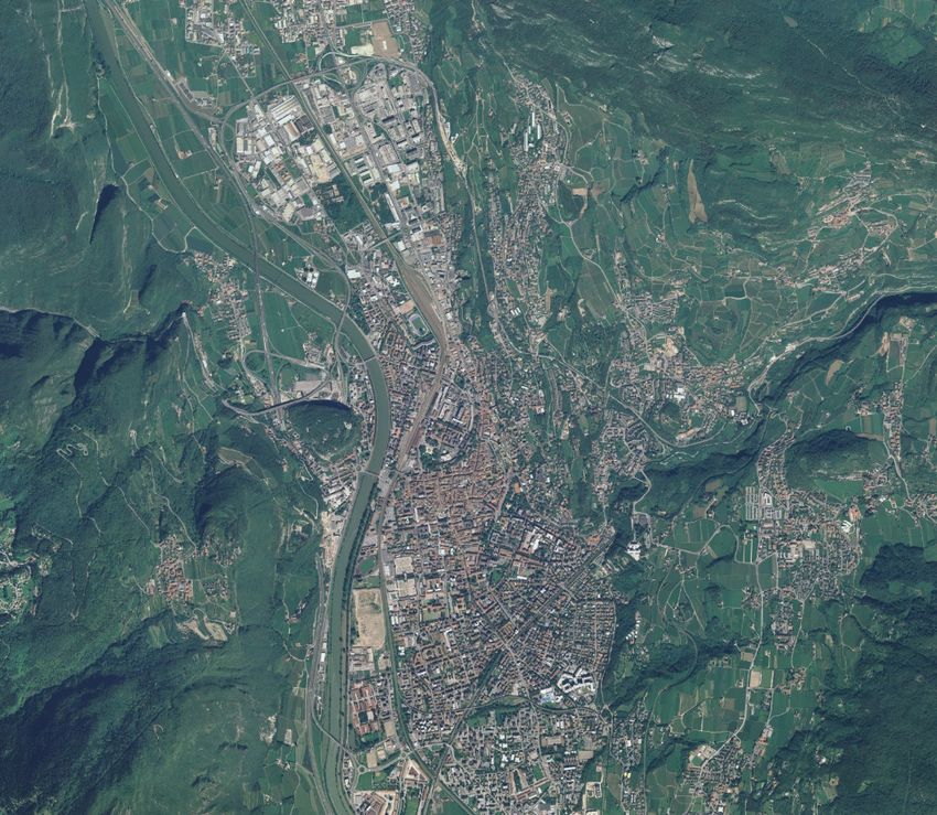
The International Archives of the Photogrammetry, Remote Sensing and Spatial Information Sciences, Volume XLII-4/W14, 2019
                             FOSS4G 2019 – Academic Track, 26–30 August 2019, Bucharest, Romania

Forest in PAT are characterized by a strong presence of conifer-        Trentino will be presented, to show how this kind of study can
ous species, mostly spruce (Servizio Fauna e Foreste, 2018).            address political and environmental decision over the conserva-
                                                                        tion of specific habitats (Ministero dell’ambiente, 2010).

                                                                                     2. MATERIALS AND METHODS

                                                                        The availability of aerial and satellite imagery in recent years
                                                                        and the development and free distribution of powerful GIS soft-
                                                                        ware made easier to perform remote sensing inquires over a
                                                                        specific territory (Rocchini et al., 2012) (Tattoni et al., 2010)
                                                                        (Neteler , Mitasova, 2008). Techniques such as image classi-
                                                                        fication are a consolidated method for studying multi-temporal
                                                                        forest evolution (Gaitanis et al., 2015) (Godone et al., 2014)
                                                                        (Gautam et al., 2004).
                                                                        Here we will briefly present the cartographic data used and the
                                                                        algorithm implemented to carry out the analysis of PAT territory
                                                                        over the years.

Figure 2. Principal forest types in PAT (Servizio Fauna e
                      Foreste, 2018)                                    2.1   The 1859 cadastrial maps

During the centuries human activities has shaped the Trentino
landscape. While activities such as timber harvesting and agri-
culture, which required to be near the townships, shaped the val-
ley bottoms, the traditional ”malga” system for pasture shaped
the high mountain meadows (MacDonald et al., 2000).
During World War I the position of Trentino was strategical for
both the Austro-Hungaric Empire and the Italian Kingdom, so
Trentino was the ground for long and weary battles. In this pe-
riod both the involved armies exploited heavily the timber, con-
tributing to the deforestation of the Alps (Tattoni et al., 2010).      Figure 3. An example of the 1859 maps: the depiction of
After World War II the socio-economical situation changed again:                         the town of Trento.
extreme poverty pushed people to leave villages in the valleys
towards the two main towns (Trento and Rovereto), abandoning
the traditional agricultural and pastoral activities, consequen-
tially abandoning meadows and crop fields to a progressive af-
forestation (De Natale et al., 2005), (Sitzia et al., 2007), (Sitzia,   The Austro-Hungaric cadastre was drawn by the Imperial edict
2009), (Tattoni et al., 2017).                                          of Franz Joseph I von Österreich in 1817. The part of PAT was
All these changes favored some types of habitats and some tree          completed in 1859 and it is divided in sheets (13300 sheets, ap-
and animal species, while other species were negatively influ-          proximately), in scale 1:2880 (Servizio Catasto della Provincia
enced by the abandonment of human activities in the moun-               Autonoma di Trento, 2019a). In 2006 the procedure of digital-
tains (Tattoni et al., 2010). The problem is not just concern-          ization and georeferentiacion of the whole cadastre was com-
ing the PAT region, but it is recognized at a European Level:           pleted. Each sheet is available in UTM32N-ETRS89 reference
the Pan-European biological and landscape diversity strategy,           system and JPG format (Servizio Catasto della Provincia Au-
the Bern Convention, the European Landscape Convention, the             tonoma di Trento, 2019b). The map represents a thematic map;
Birds and Habitats Directives are some of the acts taken by the         areas with different colours represent different land use (figure
European Union to preserve high mountain landscapes (Can-               4):
tiani et al., 2016).
In this framework it becomes crucial the knowledge of past for-
est landscape in PAT, in order to identify the evolution and the
rate of change of some specific habitats through the investigated        1.   grey for the forests;
territory (Ciolli et al., 2012). A multi-temporal map analysis           2.   light green for the private/public pastures;
was carried out in the whole Trentino territory. In part 2 we            3.   green for the crops;
will explain more in detail the features of the datasets involved,       4.   blank for the unproductive lands.
which cover a time span from 1859 to 2015. The Free and Open
Source Software for Geography GRASS GIS has been used,
exploiting its multi-purpose potential to process such a diverse
and wide variety of data, as explained in parts 2 and 4. Fo-            Water bodies, construction and roads are as well clearly recog-
cus of the current work will be given on the GRASS module               nizable and, if they are relevant, named. Information about the
used, while some already published results for limited areas of         density and type of forests are missing.

                                                 This contribution has been peer-reviewed.
                    https://doi.org/10.5194/isprs-archives-XLII-4-W14-71-2019 | © Authors 2019. CC BY 4.0 License.                    72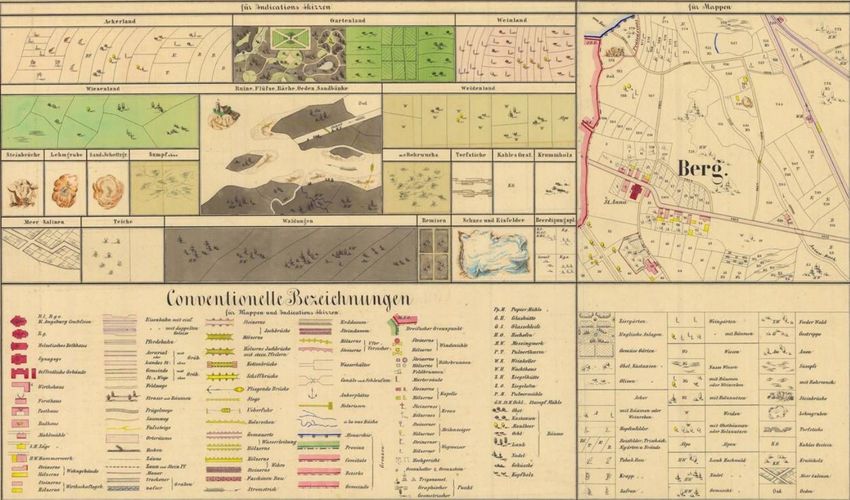
The International Archives of the Photogrammetry, Remote Sensing and Spatial Information Sciences, Volume XLII-4/W14, 2019
FOSS4G 2019 – Academic Track, 26–30 August 2019, Bucharest, Romania
2.3 The single band aerial imagery of PAT
Figure 4. The legend for the 1859 cadastrial maps (in
German).
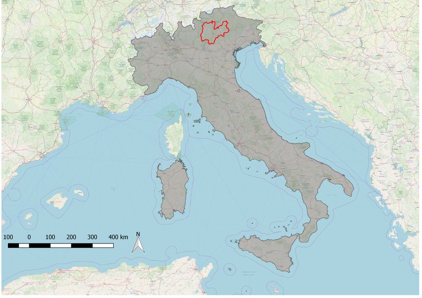
Figure 6. An example of the 1994 aerial images: the
depiction of the town of Trento.
2.2 The 1936 Italian Kingdom Forest Map
To perform the current study different sets of imagery were
chosen, in particular the images from 1954, 1973 and 1994
that are coded in single band greyscale. The set of aerial pho-
tographs from 1954 (denominated ”Volo GAI”, Gruppo Are-
The Italian Kingdom Forest Map (IKFM) was produced in 1936
onautico Italiano) in particular, has been orthorectified during
by the Milizia Italiana Forestale, to map the presence of forests
this project, as explained in part 2.6. The table 1 shows de-
in the Italian territory. The cartographic base was the map in
tails about resolution, datum and number of images used to de-
scale 1:100 000 produced by the Istituto Geografico Militare
pict PAT territory (Geoportale Provincia Autonoma di Trento,
Italiano, now available in one of the Gauss-Boaga/Rome40 da-
2019a) (Geoportale Provincia Autonoma di Trento, 2019b).
tum two zones (west and east, EPSG 3003 and 3004), depend-
ing on the map sheet location (Ferretti et al., 2018). Year Pixel dimension Images in set Datum
This map is considered the first example of forest and forest 1954 2x2m 229 WGS84- UTM32N
types mapping for the whole Italian Territory (Ferretti et al., 1973 1x1m 229 Gauss Boaga-RM40
2018). In fact the legend reports a total of 25 different forest 1994 1x1m 229 Gauss Boaga-RM40
types (Ferretti et al., 2018).
The IKFM was digitalized to be preserved and consulted freely. Table 1. Features of the greyscale sets of imagery of
Each sheet was scanned and georeferenced in a TIFF format. Trentino region, pixel dimension on the ground.
Each sheet has an approximate dimension of 112 MB, with a
resolution of 400 ppi (pixel per inch); as for the georeferencing
process it was decided to keep the original Gauss-Boaga RM40 2.4 The multi-band aerial imagery of PAT
reference system (Ferretti et al., 2018). The map has been clas-
sified and vectorized by manually digitizing each forest patch
(Ferretti et al., 2018). The resulting map is available under the
Creative commons Attribution - Version 3.0 license and can be
viewed and downloaded from a dedicated webgis (Ferretti et
al., 2019).
Figure 7. An example of the 2006 aerial images: the
depiction of the town of Trento.
Figure 5. An example of the 1936 maps: the depiction of
the town of Trento. The multi band imagery of PAT used in the current work were
taken in 2006 and 2015. Table 2 reports details about resolution,
This contribution has been peer-reviewed.
https://doi.org/10.5194/isprs-archives-XLII-4-W14-71-2019 | © Authors 2019. CC BY 4.0 License. 73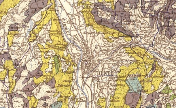
The International Archives of the Photogrammetry, Remote Sensing and Spatial Information Sciences, Volume XLII-4/W14, 2019
                                FOSS4G 2019 – Academic Track, 26–30 August 2019, Bucharest, Romania

datum and number of images used to represent PAT territory            To perform the first step it is necessary to measure and identify
(Geoportale Provincia Autonoma di Trento, 2019c) (Geoportale          the position of 4 or more fiducial markers on the original pho-
Provincia Autonoma di Trento, 2019d).                                 tograph. To perform the second step is necessary to set a con-
                                                                      sistent number of Ground Control Points, or points whose coor-
 Year       Pixel dimension    Images in set        Datum             dinates are known in both the reference systems of the original
 2006          0.5x0.5m            229          WGS84- UTM32N         image and the target reference system (Novak, 1992). Finally
 2015         0.2mx0.2m            839          WGS84- UTM32N         the re-projection is performed using a set of equations, called
                                                                      collinearity equations, which rectify the original image by shift-
  Table 2. Features of the multi-band sets of imagery of              ing, rotating and scaling each of its pixel (Novak, 1992) (Gobbi
   Trentino Territory, pixel dimension on the ground.                 et al., 2018) (Rocchini et al., 2012). A DEM which describes
                                                                      the geometry of the ground surface must be available.

These newer images have a better geometric resolution and at
least 3 bands (Red, Green and Blue). In particular the images of
2015 set include the additional near-infra-red band. The down-
side of this amount of additional information is the dimension
on the computer memory required: while the dataset of 2006
has a dimension of approximate 100 GB, the dataset of 2015
has a dimension of approximate 780 GB.

2.5     GRASS GIS

GRASS GIS has been chosen to manage and perform the im-
ages processing. The software was first developed by the U.S.
                                                                       Figure 8. Flowchart of the modules and data in GRASS
Army Construction Engineering Research Laboratories (USA-                            GIS for orthorectification.
CERL, 1982-1995). Starting from 1999 to nowadays GRASS is
released under a GNU license by the Open Source Geospatial
Foundation (OSGeo) (Neteler , Mitasova, 2008). The archi-             In this study the versions used for orthorectification are the 6.4
tecture of GRASS is inspired by a modular structure, involving        and 7.4 versions. In fact the suite i.ortho.photo was removed
more than 350 different modules, which can be stacked together        from the versions between the 6.4 and the 7.2.
to perform complex analysis (Neteler et al., 2012). Single de-        In GRASS 6.4 the process is divided in different steps:
velopers and researchers are welcome to study and develop new
modules to fit their purposes (Preatoni et al., 2012), and they
can be possibly saved in a on-line package repository, to be            1. i.target allows to chose a target reference system;
downloaded by other researchers all over the world. It is worth         2. i.ortho.elev allows to set a Digital Elevation Model used to
remembering that both the source code of GRASS and its mod-                correct the position of points according to the orography;
ules are accessible: this fact is crucial to ensure robust analysis
                                                                        3. i.ortho.camera allows to set the parameters of the camera
output (Rocchini et al., 2012) and and its suitability for educa-
                                                                           which took the picture (e.g. the focal length);
tional purposes (Ciolli et al., 2017).
Moreover, GRASS can be scripted using Python programming                4. g.gui.photo2image allows to input the position of the fidu-
language: this allows to stack different modules and apply iden-           cial markers;
tical procedures to a great number of input imagery (Van Rossum,        5. g.gui.image2target allows to input the position of the GCPs;
1995).
In the current work the versions of GRASS used are the 7.4 and          6. i.ortho.rectify performs the actual rectification.
the 6.4, as explained in part 2.6 (GRASS Development Team,
2017) (GRASS Development Team, 2018).                                 After inserting manually the position of fiducial markers and
                                                                      GCPs it was possible to use Python to apply the orthorectifi-
                                                                      cation to a whole set of imagery inside a single mapset. It is
2.6     Orthorectification of the datasets of 1954                    possible to set a raster mask: this is useful if, as it is in this
                                                                      study, the original image has a frame, containing instruments
Ortorectification is the process of adapting a flat image to a        reading, which must be removed in the orthorectified image.
rugged and curved surface, by adapting the reference and pro-         Due to the user-friendly interface, GRASS 7.4 was chosen to
jection system (Gobbi et al., 2018). In this case-study the dataset   perform the input of the GCPs: this choice was considered less
of 1954 imagery required this pre-processing because only the         time consuming than the using the old 6.4 GRASS. On the other
original images are available.                                        hand GRASS 7.4 did not allow the setting of a mask for ex-
This process is performed in three different steps:                   cluding some parts of the image (the frame, in our case study)
                                                                      therefore it was chosen to run the i.ortho.rectify command on
                                                                      GRASS 6.4.
 1. internal orientation to evaluate the position of the image
    with respect to the camera frame;
                                                                      2.7   Landuse classification algorithms
 2. external orientation to evaluate the position of the camera
    with respect to the external reference system (the chosen         To reconstruct the forest landscape it is necessary to perform a
    datum);                                                           landuse classification for each dataset. This process generates a
                                                                      map where each ”pixel” or ”object” is grouped in a finite num-
 3. orthorectification to re-project the image.                       ber of set, each one representing a type of land use. Typically

                                                  This contribution has been peer-reviewed.
                     https://doi.org/10.5194/isprs-archives-XLII-4-W14-71-2019 | © Authors 2019. CC BY 4.0 License.                  74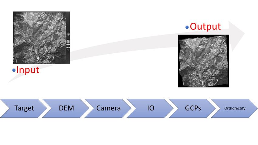
The International Archives of the Photogrammetry, Remote Sensing and Spatial Information Sciences, Volume XLII-4/W14, 2019
                             FOSS4G 2019 – Academic Track, 26–30 August 2019, Bucharest, Romania

there are 5 macro-categories: urbanized, forest, agriculture, wa-
ter, unproductive.
There are two families of algorithm: the maximum likelihood
family and the OBIA family.
The maximum likelihood algorithms require as input at least
one area for each class of landuse, where the software running
the algorithm calculates a statistical distribution of the spec-
tral response of the pixels within the area. Then each pixel of
the image is classified inside different macro-class by checking
which class its spectral response statistically belongs to (Bouman
, Shapiro, 1992).
Object-based Image Analysis (OBIA) takes a different approach:
                                                                      Figure 9. Flowchart of the modules and data in GRASS
instead than classifying each single pixel, OBIA creates groups                GIS for OBIA of multi-band images.
of pixels, called segments, which are classified as single objects
using machine learning. The parameters used by the machine
learning are the statistical distribution of the pixels radiomet-
ric response inside the single object and the geometry of the
same object (perimeter, area, compact circle, compact square,
fractal index) (Clewley et al., 2014). Each segment of pixels
is called ”object” and it is characterized by pixels with a sim-
ilar spectral response. The choice between the two algorithm
should be driven by the resolution of the input image. If the
objects (houses, trees, roads, water bodies) depicted in the im-
age are larger than the pixel resolution an OBIA approach is
more likely to give a nicer, cleaner land use output map (Bur-
nett , Blaschke, 2003). If the objects depicted are smaller than
the resolution (e.g. the resolution 30x30m of some Landsat im-       Figure 10. Flowchart of the modules and data in GRASS
ages) a maximum likelihood algorithm is preferable, because it              GIS for OBIA of single grey-band images.
is possible that similar pixels will be grouped inside the same
object while in reality they depict two different things.
In the current case study the resolution of the aerial imagery is
always smaller than the represented objects (tables 1 and 2) and     The command r.smooth.seg, applied on the single band imagery
the OBIA approach was preferred.                                     performs a preliminary segmentation on the image by smooth-
In GRASS the procedure is not coded as a suite of command            ing values of pixels within the same object and adding more
as it was for the orthorectification process, so it was necessary    contrast to the boundaries of the segments (Vitti, 2012). For this
to create a procedure which differs for the multi-band and the       reason it was considered more reliable to apply this module to
single band imagery (Grippa et al., 2017).                           the image before using i.segment. The output from i.smooth.seg
Some common steps are required:                                      was used as input to the machine learning as well.
                                                                     The procedure was scripted with Python and applied sequen-
                                                                     tially on each map inside the different datasets.

 1. i.segment performs the segmentation of the imagery;
                                                                     2.8   Manual classification of 1859 cadastrial maps

 2. r.texture r.texture evaluates the textural differences, this
    provides an additional band which give more information          The dataset of 1859 is composed by 13300 sheets, and apply-
    about each single object;                                        ing to each one of them a OBIA procedure for classifying the
                                                                     maps would have costed too much in terms of computational
                                                                     time. Instead the maps were classified using a manual proce-
 3. i.segment.stats evaluates the radiometric features of each
                                                                     dure. The procedure was performed in GRASS version 7.4 and
    segment and store them in the table associated to the (vec-
                                                                     QGIS version 2.18 (QGIS Development Team, 2019), and in-
    tor) output map;
                                                                     volved the use the vectorizer instrument.
                                                                     The vectorized areas where the ones indicated as ”forest” (with
 4. v.class.mlR uses machine learning to classify the object in-     attribute ”1” in the attribute table), ”pasture” (with attribute ”2”
    side the chosen land-use categories;                             in the attribute table) and ”wooded pasture” (with attribute ”3”
                                                                     in the attribute table). A few simple rules were followed:

Figures 10 and 9 show the flowchart with the input data for the       1. if two or more neighbour cadastrial parcel had the same
case of single band imagery (1954, 1973, 1994) and colour im-            landuse they were digitized as one single area;
agery (2006, 2015). The textural measure was considered in
both cases as additional image band, because where it is neces-       2. assign a single identifier value to each area;
sary to discriminate between forests and crop fields the spectral     3. digitize following the black border of each area and in-
response is similar, but the textural measure within the same            clude the border in the area;
object differs, giving to the machine learning algorithm helpful
data to discriminate the two situations (Haralick et al., 1973).      4. exclude lakes and rivers from the digitalization process.

                                                This contribution has been peer-reviewed.
                   https://doi.org/10.5194/isprs-archives-XLII-4-W14-71-2019 | © Authors 2019. CC BY 4.0 License.                     75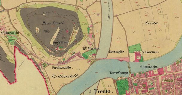
The International Archives of the Photogrammetry, Remote Sensing and Spatial Information Sciences, Volume XLII-4/W14, 2019
                             FOSS4G 2019 – Academic Track, 26–30 August 2019, Bucharest, Romania

 Year             Denomination                 Scale         Type of map        Pixel dimension     Dimension [GB]             Datum
 1859       Theresiascher Kadastrte           1:1440       Topographic map          0.2x0.2               20             ETRS89-UTM32N
 1936     Italian Kingdom Forest Map        1:100000       Topographic map         0.32x0.32               1             Gauss Boaga RM40
 1954               Volo GAI                 1:35000      Aerial images BN           2x2m                  8             WGS84- UTM32N
 1973           Volo Rossi-EIRA              1:10000      Aerial images BN           1x1m                  8             Gauss Boaga-RM40
 1994              Volo Italia               1:10000      Aerial images BN           1x1m                  8             Gauss Boaga-RM40
 2006            Volo Terraitaly              1:5000      Aerial images RGB        0.5x0.5m              100             WGS84-UTM32N
 2015              Volo AGEA                  1:5000      Aerial images RGB        0.2x0.2m              730             WGS84-UTM32N

                                      Table 3. The data collection for the current case-study.

                         3. RESULTS                                    provides an efficient way of finding an optimum set of parame-
                                                                       ters of the land use classification procedure. The classification
A complete dataset The current work is leading to create to            of the complete Trentino territory using OBIA is under way for
a complete collection of maps and aerial imagery of Provin-            all the available datasets whith a scripted batch procedure. The
cia Autonoma di Trento, with a timespan of 160 years. In the           effectiveness of this classification OBIA approach will be tested
perspective of study whose objective is to analyse landscape           comparing the results with those obtained in the previous works
changes over the years having a complete dataset is a crucial          (Cattani, 2015) (Tattoni et al., 2010) (Maimeri, 2018) with the
results for the future of the work. The collected imagery cov-         OBIA approach.
ers the whole territory of Trentino, with a high-resolution and        Finally, the use of QGIS and its digitizing tools plugin pre-
detailed scale, as shown in table 3.                                   vented topological errors in the digitalization process of the
                                                                       1859 dataset, assuring that the created vector files were viable
1859 maps A partial result is the digitalization of the 1859           for further analysis.
cadastrial maps. By following the rules explained in section 2.8
areas of forests and open pastures were classified for the whole       The future of the research In the current study, the recon-
region of Trentino.                                                    struction of the past forest landscape from landuse classifica-
                                                                       tion will be used for landscape and ecosystem services analysis
Orthorectification of the 1954 dataset A total amount of 92            (Ciolli et al., 2019). Following (Ciolli et al., 2012) and (Tat-
aerial imagery of the dataset of 1954 aerial images were col-          toni et al., 2010), the landuse maps will be used to evaluate
lected and orthorectified, integrating the imagery of (Cattani,        landscape metrics using Fragstat or the LeCos suite in QGIS to
2015) (Tattoni et al., 2010) (Rocchini et al., 2012) (Maimeri,         evaluate parameters that can describe how the forest coverage
2018) was possible to achieve a complete rectified set of im-          has changed during the years. Metrics such as the mean forest
agery from the 1954 dataset for the whole PAT (Gobbi et al.,           patch area, for instance, can represent how the forests became
2018).                                                                 more fragmented or compact. This information helps to give an
                                                                       overall view on the fluctuation of the total forest coverage and
Testing the OBIA procedure The OBIA procedure has been                 its density (Campagnaro et al., 2017) (Tattoni et al., 2017) and
calibrated and applied to the whole variety of aerial imagery in       it will be crucial for mapping the hydro-geological risk (Ciolli
the dataset. This result is important because accomplish one of        et al., 2019).
the aims of this project, i.e. to automatize the classification pro-   The second field of application of the forest coverage data is
cess as much as possible so that its application to large datasets     the use of predictors such as Markov Chains to simulate how
covering the whole Trentino region is feasible (Tattoni et al.,        protected habitats will evolve if the ”no human intervention”
2010) (Cattani, 2015) (Maimeri, 2018). The synergy between             policy is applied, as specified in (Ciolli et al., 2012).
Python and GRASS rendered possible to automatize the OBIA              A total of 142 Sites of Community Importance have been recog-
in just 140 lines of code.                                             nized in Trentino: the fate of this areas can be easily protected
                                                                       by human intervention and this study can help to program the
                                                                       actions that can be performed to protect such areas.
          4. DISCUSSION AND CONCLUSIONS

The use of GRASS and QGIS In the course of this research
the main tool has been GRASS. The availability of GRASS
source code under the GPL was useful especially in the or-
thorectification phase, where it was crucial to understand how
the errors in the GCPs were calculated, accessing the source
code of the suite for orthorectification gave insight to the inter-
                                                                                         ACKNOWLEDGMENTS
pretation of the errors (Gobbi et al., 2018). As a matter of fact
the two version of GRASS used (6.4 and 7.4) such errors were
displayed with two different methods, and understand which             We would gladly thank Luca Delucchi from Fondazione Ed-
one was more significant required accessing to the source code.        mund Mach for the help with GRASS, in particular with the
The possibility to script GRASS with Python is a major advan-          module for the orthorectification. All the aerial imagery were
tage in managing large datasets (in terms of number of elements        provided by the Provincia Autonoma di Trento, while the cadaster
and dimension in GB, see table 3). Once the input parameters           historical map for the Province of Trento has been made avail-
are set for a specific analysis, the same module can be sequen-        able by the Servizio Catasto della Provincia Autonoma di Trento,
tially applied to different images with the same parameters. It        under the Creative Commons Attribution 4.0 license.
was possible to apply the same modules sequence in the OBIA            Finally we would like to thank the Ufficio Fauna e Foreste, in
procedure with different input parameters with minimum inter-          the person of Maurizio Miori for providing all the data about
vention from the user by scripting the algorithm. This approach        forest types in Trentino.

                                                 This contribution has been peer-reviewed.
                    https://doi.org/10.5194/isprs-archives-XLII-4-W14-71-2019 | © Authors 2019. CC BY 4.0 License.                   76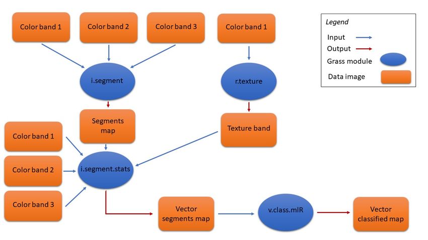
The International Archives of the Photogrammetry, Remote Sensing and Spatial Information Sciences, Volume XLII-4/W14, 2019
                             FOSS4G 2019 – Academic Track, 26–30 August 2019, Bucharest, Romania

                         REFERENCES                                      Gaitanis, A, Kalogeropoulos, K., Detsis, V., Chalkias,
                                                                         C., 2015. Monitoring 60 Years of Land Cover Change
Bouman, C., Shapiro, M., 1992. Multispectral Im-                         in the Marathon area, Greece. Land, 4, 337–354.
age Segmentation using a Multiscale Image Model.                         https://doi.org/10.3390/land4020337.
Proceedings of IEEE International Conference on
Acoustoustic,      Speech and Sig. Proc.,     565–568.                   Gautam, A.P., Shivakoti, G.P., Webb, E.L., 2004. Forest cover
http://dx.doi.org/10.1109/ICASSP.1992.226150.                            change, physiography, local economy, and institutions in a
                                                                         mountain watershed in Nepal. Environment Managment, 1, 48–
Burnett, C, Blaschke, T., 2003. A multi-scale segmenta-                  61. https://doi.org/10.1007/s00267-003-0031-4.
tion/object relationship modelling methodology for landscape
analysis. Ecological Modelling, 168, 233–249.                            Geoportale Provincia Autonoma di Trento, 2019a. Metadati
                                                                         volo 1973. tn:8cf5ffba-f738-4e60-a0e6-7669919eec24. Ac-
Campagnaro, T., Frate, L., Carranza, M.L., Sitzia, T., 2017.             cessed: 2019-04-29.
Multi-scale analysis of alpine landscapes with different intensi-
ties of abandonment reveals similar spatial pattern changes: im-         Geoportale Provincia Autonoma di Trento, 2019b. Metadati
plication for habitat conservation. Ecological Indicators, 147–          volo 1994. tn:629ccdc8-e046-411c-95b0-326cb0bdc656. Ac-
159. https://doi.org/10.1016/j.ecolind.2016.11.017.                      cessed: 2019-04-29.
                                                                         Geoportale Provincia Autonoma di Trento, 2019c. Metadati
Cantiani, M.G., Geitner, C., Haida, D., Maino, F., Tat-
                                                                         volo 2006. tn:a1dfd067-1f7d-40d1-b873-fc665a61af6b. Ac-
toni, C., Vettorato, D., Ciolli, M., 2016. Balancing eco-
                                                                         cessed: 2019-04-29.
nomic development and environmental conservation for a
new governance of Alpine areas. Sustainability, 802–820.                 Geoportale Provincia Autonoma di Trento, 2019d. Metadati
http://dx.doi.org/10.3390/su8080802.                                     volo 2015. tn:f2e88f1b-05d9-4942-93ee-857a0a9e1f0b. Ac-
                                                                         cessed: 2019-04-29.
Cattani, G., 2015. Metodologia per la valutazione della perdita
di biodiversità dovuta al cambiamento del paesaggio agrofore-           Gobbi, S., Maimeri, G., Tattoni, C., Cantiani, M.G., Roc-
stale: il caso del tesino. Master’s thesis, University of Trento.        chini, D., La Porta, N., Ciolli, M., 2018. Orthorectification
                                                                         of a large dataset of historical aerial images:procedure and
Ciolli, M., Bezzi, M., Comunello, G., Laitempergher, G.,
                                                                         precision assessment in an open source environment. The In-
Gobbi, S., Tattoni, C., Cantiani, M.G., 2019. Integrating
                                                                         ternational Archives of the Photogrammetry, Remote Sens-
dendrochronology and geomatics to monitor natural haz-
                                                                         ing and Spatial Information Sciences, XLII-4/W8, 53–59.
ards and landscape changes. Applied Geomatics, 11, 39–52.
                                                                         https://doi.org/10.5194/isprs-archives-XLII-4-W8-53-2018.
https://doi.org/10.1007/s12518-018-0236-0.
                                                                         Godone, D., Gabarino, M., Sibona, E., 2014. Progressive
Ciolli, M., Federici, B., Ferrando, I., Marzocchi, R., Sguerso,
                                                                         fragmentation of a traditional Mediterranean landscape by
D., Tattoni, C., Vitti, A., Zatelli, P., 2017. FOSS tools and ap-
                                                                         hazelnut plantations: The impact of CAP over time in
plications for education in geospatial sciences. ISPRS Interna-
                                                                         the Langhe region (NW Italy). Land use Policy, 48–61.
tional Journal of Geo-Information, 6.
                                                                         https://doi.org/10.1016/j.landusepol.2013.08.018.
Ciolli, M., Tattoni, C., Ferretti, F., 2012. Understanding               GRASS Development Team, 2017. Geographic Resources
forest changes to support planning: A fine-scale Markov                  Analysis Support System (GRASS) Software, Version 6.4.
chain approach. in F. Jordán, S. Jorgensen (edited by), Mod-            Open Source Geospatial Foundation. grass.osgeo.org (1
els of the ecological hierarchy from molecules to the eco-               November 2017).
sphere. Elsevier, Amsterdam. http://dx.doi.org/10.1016/B978-
0-444-59396-2.00021-3.                                                   GRASS Development Team, 2018. Geographic Resources
                                                                         Analysis Support System (GRASS) Software,Version 7.4. Open
Clewley, D., Bunting, P., Shepherd, J., Gillingham, S.,                  Source Geospatial Foundation. grass.osgeo.org (20 September
Flood, N., Dymond, J., Lucas, R., Armston, J., Moghad-                   2018).
dam, M., 2014. A Python-Based Open Source System for
Geographic Object-Based Image Analysis (GEOBIA)utilizing                 Grippa, T., Lennert, M., Beaumont, B., Vanhuysse,
raster attribute tables. Remote sensing, 6, 6111–6135.                   S., Stephenne, N., Wolff, E., 2017. An Open-Source
https://doi.org/10.3390/rs6076111.                                       Semi-Automated Processing Chain for Urban Object-
                                                                         Based Classification. Remote Sensing, 4, 358–378.
De Natale, F., Gasparini, P., A., Carriero, 2005. A study on tree        https://doi.org/10.3390/rs9040358.
colonization of abandoned land in the Italian Alps: extent and
characteristics of new forest stands in Trentino. Proceedings of         Haralick, R. M., Shanmugam, K., Dinstein, I., 1973. Textu-
the IUFRO Congress Sustainable forestry in theory and prac-              ral features for image classification. IEEE transactions on sys-
tice.                                                                    tems,man and cybernetics, 3, 610–621.
Ferretti, F., Sboarina, C., Tattoni, C., Vitti, A., Zatelli, P.,         MacDonald, D., Crabtree, J., Wiesinger, G., Dax, T., Stamou,
Geri, F., Pompei, E., Ciolli, M., 2018. The 1936 Italian King-           N., Fleury, P., Lazpita, J., Gibon, A., 2000. Agricultural aban-
dom Forest Map reviewed: a dataset for landscape and eco-                donment in mountain areas of Europe: environmental conse-
logical research. Annals of Silvicultural Research, 42, 3–19.            quences and policy response. Journal of Environmental Man-
https://doi.org/10.12899/asr-1411.                                       agement, 59, 47–69. https://doi.org/10.1006/jema.1999.0335.
Ferretti, F., Sboarina, C., Tattoni, C., Vitti, A., Zatelli, P., Geri,   Maimeri, G., 2018. Variazione della copertura forestale in val
F., Pompei, E., Ciolli, M., 2019. Carta forestale del regno di           di fassa tramite analisi gis multitemporale. Master’s thesis, Uni-
italia. http://carta1936.dicam.unitn.it. Accessed: 2019-04-29.           versity of Trento.

                                                 This contribution has been peer-reviewed.
                    https://doi.org/10.5194/isprs-archives-XLII-4-W14-71-2019 | © Authors 2019. CC BY 4.0 License.                      77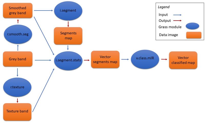
The International Archives of the Photogrammetry, Remote Sensing and Spatial Information Sciences, Volume XLII-4/W14, 2019
                             FOSS4G 2019 – Academic Track, 26–30 August 2019, Bucharest, Romania

Ministero dell’ambiente, 2010. Elenco ufficiale delle aree pro-     Vitti, A., 2012. The Mumford-Shah variational model for image
tette (euap). Sixth update, approved the 27th of April 2010, pub-   segmentation: An overview of the theory, implementation and
lished in the official Gazette (125).                               use. ISPRS Journal of Photogrammetry and Remote Sensing,
                                                                    69, 50–64. https://doi.org/10.1016/j.isprsjprs.2012.02.005.
Neteler, M., Bowman, M.H., Landa, M., Metz, M.,
2012. GRASS GIS: A multi-purpose open source GIS.
Environmental Modelling and Software, 31, 142–130.
https://doi.org/10.1016/j.envsoft.2011.11.014.

Neteler, Makus, Mitasova, Helena, 2008. Open Source GIS: A
GRASS GIS Approach. Springer, New York.

Novak, Kurt, 1992. Rectification of Digital Imagery. Pho-
togrammetric Engeneering and Remote Sensing, 58, 339–344.

Preatoni, D.G., Tattoni, C., Bisi, F., Masseroni, E.,
D’Acunto, D., Lunardi, S., Grimod, I., Martinoli, A.,
Tosi, G., 2012. Open source evaluation of kilometric
indexes of abundance. Ecological Informatics, 35–40.
http://dx.doi.org/10.1016/j.ecoinf.2011.07.002.

QGIS Development Team, 2019. QGIS Geographic Informa-
tion System, version 2.18. Open Source Geospatial Foundation.

Rocchini, Duccio, Metz, Markus, Frigeri, Alessandro, Deluc-
chi, Luca, Marcantonio, Matteo, Netler, Markus, 2012. Ro-
bust rectification of aerial photographs in an open source
environment. Computers and geosciences, 39, 145–151.
https://doi.org/10.1016/j.cageo.2011.06.002.

Servizio       Catasto     della      Provincia       Autonoma
di     Trento,     2019a.    History      of     the    cadaster
historical     map     for   the     Province      of    Trento.
http://www.catasto.provincia.tn.it/cenni storici/pagina8.html.
Accessed: 2019-04-29.

Servizio Catasto della Provincia Autonoma di Trento,
2019b.    Mappe      storiche   di    impianto (urmappe).
https://www.catastotn.it/mappeStoriche.html.    Accessed:
2019-04-29.

Servizio Fauna e Foreste, 2018. Schede dei tipi forestali, carat-
teristiche e indicazioni gestionali. 1st edn, Provincia Autonoma
di Trento, Trento, Via Trener 3.

Sitzia, T., 2009. Ecologia e gestione dei boschi di neofor-
mazione nel paesaggio trentino. Servizio Foreste e Fauna,
Provincia Autonoma di Trento, Trento, Italy. pp. 301.

Sitzia, T., Carriero, A., De Natale, F., Gasparini, P., Wolynski,
A., Viola, F., 2007. Recent secondary woodlands in a regional
sample of southern-alpine abandoned landscapes: implications
for restoration ecology and silviculture. Proceedings of the sev-
enth IALE World Congress, 2, 783–784.

Tattoni, C, Ciolli, M, Ferretti, F, Cantiani, M.G., 2010.
Monitoring spatial and temporal pattern of Paneveggio for-
est ( northern Italy ) from 1859 to 2006. iForest, 3, 72–80.
https://doi.org/10.3832/ifor0530-003.

Tattoni, C., Ianni, E., Geneletti, D., Zatelli, P., Ciolli,
M., 2017. Landscape changes, traditional ecological knowl-
edge and future scenarios in the Alps: A holistic eco-
logical approach. Science of the Total Environment, 27–36.
http://dx.doi.org/10.1016/j.scitotenv.2016.11.075.

Van Rossum, G., 1995. Python Library Reference. CWI Report.

                                                This contribution has been peer-reviewed.
                   https://doi.org/10.5194/isprs-archives-XLII-4-W14-71-2019 | © Authors 2019. CC BY 4.0 License.               78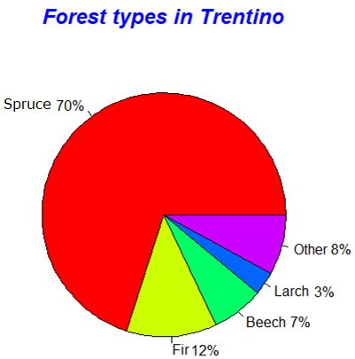
You can also read