GPU-Powered Spatial Database Engine for Commodity Hardware: Extended Version - arXiv
←
→
Page content transcription
If your browser does not render page correctly, please read the page content below
GPU-Powered Spatial Database Engine for Commodity Hardware:
                                                                  Extended Version
                                                                           Harish Doraiswamy1 and Juliana Freire2
                                                                                   1
                                                                                   Microsoft Research India
arXiv:2203.14362v1 [cs.DB] 27 Mar 2022

                                                                              harish.doraiswamy@microsoft.com
                                                                                     2
                                                                                       New York University
                                                                                    juliana.freire@nyu.edu

                                                                                              Abstract
                                                    Given the massive growth in the volume of spatial data, there is a great need for systems that can
                                               efficiently evaluate spatial queries over large data sets. These queries are notoriously expensive using
                                               traditional database solutions. While faster response times can be attained through powerful clusters or
                                               servers with large main-memory, these options, due to cost and complexity, are out of reach to many data
                                               scientists and analysts making up the long tail.
                                                    Graphics Processing Units (GPUs), which are now widely available even in commodity desktops and
                                               laptops, provide a cost-effective alternative to support high-performance computing, opening up new op-
                                               portunities to the efficient evaluation of spatial queries. While GPU-based approaches proposed in the
                                               literature have shown great improvements in performance, they are tied to specific GPU hardware and
                                               only handle specific queries over fixed geometry types.
                                                    In this paper we present SPADE, a GPU-powered spatial database engine that supports a rich set
                                               of spatial queries. We discuss the challenges involved in attaining efficient query evaluation over large
                                               datasets as well as portability across different GPU hardware, and how these are addressed in SPADE. We
                                               performed a detailed experimental evaluation to assess the effectiveness of the system for wide range of
                                               queries and datasets, and report results which show that SPADE is scalable and able to handle data larger
                                               than main-memory, and its performance on a laptop is on par with that other systems that require clusters
                                               or large-memory servers.

                                         1    Introduction
                                         The widespread use of GPS-based sensors, IoT devices, phones and social media has resulted in an explosion
                                         of spatial data that is being collected and stored. Increasingly, data scientists and analysts are resorting to
                                         interactive analyses and visual tools to obtain insights from these data (e.g., [4, 5, 14, 15, 40]). However,
                                         executing queries involving complex geometric constraints over large spatial data sets is time consuming,
                                         and this greatly hampers users’ ability to interactively explore data. Commonly-used approaches, such as
                                         the spatial extensions available in existing relational database systems, even on powerful hardware, take from
                                         several minutes to run a single spatial selection query [12] to several hours for more complex queries such as
                                         joins [33]. While faster response times can be attained through powerful clusters and large memory servers,
                                         these options, due to cost and complexity, are often out of reach for analysts that make up the long tail; they
                                         are forced to work with small subsets of the data that can be handled in less powerful desktops and laptops.
                                         This raises an important question: can we support scalable spatial analytics for users in the long tail?
                                            Modern graphics processing units (GPU) exhibit impressive computational power and provide a cost-
                                         effective alternative to support high-performance computing. For example, the Intel UHD GPU present in

                                                                                                  1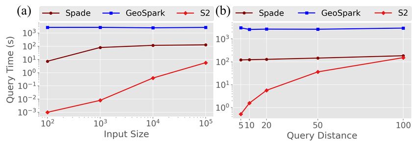
mid-range laptops reaches up to 0.5 TFLOPS, while the previous generation Nvidia GTX 1070 MaxQ mobile
GPU reaches over 5 TFLOPS. Current-generation desktop and server GPUs are even faster, attaining speeds
as high as 36 TFLOPS. Their wide availability, even in lower-end laptops, open up new opportunities to de-
mocratize large-scale spatial analytics. Not surprisingly, methods have been proposed to evaluate different
types of spatial queries on the GPU [8, 12, 41, 49–51]. However, their adoption has not expanded beyond
select research projects. We posit that this is due to two main reasons. First, no single system or library can
both harness the power offered by GPUs and support the variety of queries commonly used in spatial analysis.
Second, almost all current approaches use CUDA [26] and only work on Nvidia GPUs which are not always
available in commodity hardware.
   One possible approach would be to design a full-fledged GPU-based spatial query engine that combines
existing approaches. But such a strategy quickly becomes unwieldy because existing methods target specific
queries (e.g., selection over point data, or aggregation over polygons) and use custom data structures/indexes
for each query type. This makes it difficult to reuse the data structures across different queries. Moreover,
many of these approaches port CPU-based algorithms to the GPU. While general-purpose computing capa-
bilities of GPUs have improved in recent times, traditional algorithmic constructs still cannot make optimal
use of the parallelization provided by them, often leading to ineffective use of GPU capabilities.
The Spade Query Engine. To overcome these challenges, we propose Spade, a GPU-powered spatial
query engine. By adopting the canvas data model and GPU-friendly algebra [10], Spade is able to support
a rich set of query types. In addition, since the algebraic operators are adapted from common computer
graphics operations for which GPUs are optimized, it is possible to harness the compute power provided by
the hardware. Spade uses the computer graphics pipeline to implement the operators, and thus, it is portable
and can be run on any GPU hardware.
   There are several challenges involved in implementing the GPU-friendly algebra and data model to effi-
ciently handle large spatial data sets on commodity hardware. First, the system must support datasets that do
not fit in main memory. While the implementation of some of the algebra operators is straightforward, for
others a naı̈ve implementation leads to performance bottlenecks and the inability to handle large data due to
memory limitations of the GPU. In addition, these operators involve costly geometric tests whose computa-
tional complexity is polynomial to the size of the geometries, and thus can negatively impact query execution
time.
   To design Spade, we adopted a computer-graphics perspective to evaluate spatial queries. We devised a
methodology to implement the GPU-friendly operators [10] using the modern graphics pipeline [37], which
enables both portability and efficiency. We show that, by using the GPU-based operators to efficiently query
spatial indexes, Spade is able to handle large data sets that do not fit in memory. We also propose two
canvas-specific indexes that both speed up geometry intersections and improve GPU occupancy.
   Spade is designed to seamlessly support linkage to relational data and to be easily integrated with re-
lational database systems. This is crucial since analytics over spatial data often requires a combination of
relational and spatial queries. Spade also includes a query optimizer that specifies the order of operations
for a given query plan and chooses the appropriate index and/or implementation for the different operators.
   To assess the performance of Spade and its ability to handle large-scale analytics on commodity desktops
and laptops, we perform an extensive evaluation using a wide range of queries and real data sets having as
many as 100 million polygons and 2 billion points. The results show that Spade is scalable and efficiently
handles data that is larger than main memory and that its performance is comparable to that of cluster-based
and large memory solutions. Specifically, Spade running on a laptop equipped with a Nvidia 1070 MaxQ
GPU performs on par with both GeoSpark [48] running on a 17 node cluster, as well as in-memory spatial
libraries [17] running on large main-memory servers. We also discuss insights uncovered during the evaluation
into how to further improve Spade as well as how to combine it with the existing solutions.

                                                      2
Contributions. We introduce Spade which, to the best of our knowledge, is the first GPU-powered spatial
database engine that supports the evaluation of a rich set of spatial queries over different GPU hardware.
Given its ability to efficiently handle complex queries over big data on commodity hardware, Spade has the
potential to make large-scale spatial data analysis widely accessible. To summarize:
• We demonstrate how the canvas model and the spatial algebra [10] can be realized using the computer
graphics pipeline to attain efficiency, accuracy, portability, and scalability on commodity hardware.
• We propose two indexes designed to support the canvas model: the boundary index that enables constant
time geometry intersection tests, and the layer index that speeds up spatial join queries by improving the
GPU occupancy.
• We describe the architecture and implementation of the Spade system and show how it can be integrated
with existing relational systems, how existing disk-based spatial indexes can also be queried using the GPU
operators, and how query execution can be optimized.
• We present results of an extensive experimental evaluation of Spade which demonstrate its efficiency.
2 Background
To provide context we first give a brief informal overview of the canvas data model and GPU-friendly spatial
algebra [10]. We refer the reader to [10, 11] for details. We then describe the shader-based computer graphics
pipeline [37] that is used to implement Spade.
2.1 Spatial Data Model and Algebra
The canvas data model and GPU-friendly algebra [10] were designed to exploit GPUs for executing spatial
queries. Intuitively, the canvas data model [10] can be thought of as a “drawing” of the geometry, and is
represented as a collection of images. However, unlike traditional images, each pixel of a canvas model image
is designed to store the necessary metadata to both identify the geometry it represents as well as to support
query execution. This model provides a uniform representation for spatial objects – not only points, lines, and
polygons, but also any combination of these primitives.
The main advantage of the above representation is that it naturally allows the parallel execution of the GPU-
friendly operators defined by the algebra. In particular, the algebra consists of five fundamental operators,
inspired by common computer graphics operations. Figure 3 illustrates the operators implemented in Spade.
1. Geometric Transform: moves geometric objects in space.
2. Value Transform: modifies a geometric object’s properties.
3. Mask: filters regions based on a given mask condition.
4. Blend: merges two canvases into one.
5. Dissect: splits a canvas into a collection of non-empty canvases.
In addition to these, the algebra also includes derived operators that are compositions of one or more
fundamental operators. These include the Multiway Blend operator, that applies several blends to merge
multiple canvases, and the Map operator that is a composition of a dissect followed by a geometric transform.
Spatial queries are realized by composing one or more of the above operators. For example, consider the
spatial selection query that selects all geometric objects intersecting a polygonal constraint. This is realized by
first blending the canvas corresponding to a geometric object with the canvas representing the query polygon,
and then applying the mask operator that removes objects outside the query polygon. The first step creates an
image that merges the query polygon and the input geometry into a single canvas, and the second step removes
any geometry that is present outside the query polygon. The non-empty canvases that remain after the above
3two operations correspond to the query results. Note that the above composition of operators work on any
geometric primitive. As described in Section 5.2, other spatial queries can be realized in a similar fashion.
2.2 The Computer Graphics Pipeline
Graphics intensive applications, such as games, involve rendering complex scenes that continuously change
based on end-user interactions. These scenes are rendered as a collection of frames, where each frame contains
the geometric objects as seen from a camera at a given time stamp. To obtain smooth transitioning between
the frames, it is critical to have a high frame rate, i.e., a large number of frames rendered per second. GPUs
are designed to speedup precisely these operations which are executed through the computer graphics pipeline
– a high-level interface that allows the use of the underlying GPU hardware, while the GPU drivers handle
low-level tasks such as optimizing for the GPU architecture (e.g., handling rasterization, threads).
OpenGL [37] (cross platform), Direct3D [24] (Microsoft Windows), metal [23] (OSX), and the more recent
Vulkan [20] (cross platform) are some of the popular application programming interfaces (API) that support
the computer graphics pipeline. This pipeline (also known as the shader pipeline) is divided into a set of
stages that can be customized by the developer through the use of shaders.
Vertex Shader. The first stage of the pipeline is used to process the set of individual vertices that form
the geometric primitives to be rendered. It supports three types of geometric primitives—points, lines and
triangles (polygons are rendered as a collection of triangles). This stage is used to convert vertex coordinates
into a common screen space (the coordinate system w.r.t. the camera), known as model-view-projection.
Custom Geometry Creation. This is an optional stage which is used to create custom geometries. Either the
tessellation shader or the geometry shader can be used for this purpose. This stage takes as input the vertices
output from the vertex shader together with optional user-defined parameters, and outputs zero or more new
geometric primitives.
Vertex Post Processing. This stage is handled by the GPU (driver) and is used for clipping and rasterization.
Clipping is the process where primitives outside the viewport (the space corresponding to the region visible
from the camera) are removed, while those (lines and triangles) that are partially outside are cropped resulting
in a new set of primitives that are fully contained within the viewport.
Rasterization is the process that converts each primitive within the viewport into a collection of fragments.
Here, a fragment can be considered as the modifiable data corresponding to a pixel. The fragment size
therefore depends on the resolution (width and height in terms of the number of pixels that form the screen
space). Given the crucial part it plays in the graphics pipeline, GPU hardware vendors optimize parallel
rasterization by directly mapping computational concepts to the internal layout of the GPU. Since all the
primitives are simple (lines or triangles), identifying fragments that form a given primitive is amenable to
hardware implementation.
Fragment (or Pixel) Shader. This stage allows custom processing for each fragment that is generated by
the rasterizer. It is typically used to compute and set the “color” and “depth” (distance from the camera) for
the fragment. Depending on the required functionality, it can also be used for other purposes (e.g., to discard
fragments, write to additional output buffers).
Post Fragment Processing. The final stage of the pipeline processes the individual fragments output from
the fragment shader to generate the pixels of the image corresponding to the scene being rendered. It is
responsible for performing actions such as alpha blending (when objects have translucent material, then the
colors of obstructing objects are blended together based on a blend function).
Virtual Screen. Graphics APIs also allow results to be output to a “virtual” screen, which is represented using
a frame buffer (also called frame buffer object or FBO). Thus, rendering can now be performed without the
4Figure 1: Spade system architecture.
need of a physical monitor. Even though the resolutions supported by existing monitors are limited, current
generation graphics hardware supports frame buffers with resolutions as large as 32K × 32K.
Each pixel of this FBO is represented by 4 values [r, g, b, a], corresponding to the red, blue, green, and
alpha color channels. Each FBO is associated with a texture that stores the actual image.
3 SPADE: System Overview
The architecture of Spade, shown in Fig. 1, consists of four main components which we describe below. Note
that since Spade is implemented using the computer graphics pipeline, it can run on any GPU hardware.
Relational Data Store. All data, indexes, and meta-data used by Spade are stored as relational tables. For
our initial implementation, we use the embedded column store MonetDBLite [35] which provides a simple C
API to load and store data using SQL. However, since the data is accessed using SQL, it is straightforward to
integrate Spade with other database systems.
Discrete Canvas Creation. This component is responsible for creating canvases – the data used by the spatial
operators. In Section 4, we outline how a discrete canvas can be created using the shader pipeline, and describe
how to ensure accurate queries in spite of using rasterization to generate this canvas. Spade supports data
sets comprising of common geometric primitives—points, lines, and polygons1 .
Spatial Query Engine. The spatial query engine, described in Section 5, forms the core of Spade and is
responsible for planning, optimization, and execution of spatial queries.
Index Manager. Spade maintains two types of indexes that are used during the execution of spatial queries:
1. Canvas-specific indexes speed up spatial intersection tests and reduce the number of canvases that are
created respectively, thus making spatial operations on the GPU more efficient (see Section 4.3).
2. The disk-based index supports out-of-core queries – the current version of Spade stores the underlying
spatial data using a clustered grid index. However, as discussed in Section 7, other indexing strategies can be
easily integrated with Spade.
4 Discrete Canvas
The canvas, when rasterized by the GPU, can lead to inaccurate query results. To overcome this limitation, we
formalize the notion of discrete canvas in Section 4.1 and describe its creation using the rasterization-based
1
wlog., lines and polygons are used to denote polylines and multi-polygons.
5pipeline in Section 4.2. Finally, in Section 4.3, we introduce canvas-specific indexes that we designed to
speedup query processing.
4.1 Rasterized Canvas Representation
Using the rasterization-based pipeline, the Euclidean space is divided into a set of pixels. Thus, a trivial
implementation of the canvas would have each pixel map to the necessary metadata. This metadata is defined
as a triple of triples (or a 3 × 3 matrix) [10], where each triple stores information corresponding to the three
primitive types (point, line, polygon) respectively, that makeup a geometric object. However, this would result
in inaccuracies due to the discretization caused by rasterization: since a pixel need not lie entirely within a
geometry, this would induce errors for pixels that partially intersect the geometry.
We therefore extend the formal model from [10] to define a discrete canvas that uses a triple of 4-tuples(or
a 3 × 4 matrix). Here, for each 4-tuple (v0 , v1 , v2 , vb ), v0 , v1 , and v2 are the same as in the original definition,
and vb stores the necessary boundary data – a pointer to the boundary index that is used to obtain accurate
query results (see Section 4.3). Intuitively, the discrete canvas can be thought of as a “localized” grid index
corresponding to each geometric object. As mentioned earlier, each pixel of the texture associated with an
FBO can store 4 values corresponding to the 4 color channels—this 4-tuple directly maps to the color channels
of a pixel. Thus, to represent the canvas on the GPU, we use 3 textures, one for each primitive type.
4.2 Canvas Creation
Spade uses canvases to represent both data and query constraints. In our implementation, instead of storing
all canvases associated with a data set, we create them on the fly as needed. The advantages of this approach
are twofold. First, the data can be stored in the database in its vector format, thus reducing the space overhead.
Second, depending on the query constraints, it is possible to realize the canvas for only a subset/sub-region of
the data, often making it more efficient to render than load a pre-stored canvas. This is because the memory
overhead of the serialized canvas is typically much higher, making it more costly to transfer the data from
CPU to GPU as compared to data stored in a vector format. In what follows, we describe how canvases are
created for different types of geometries.
Canvases for Traditional Primitives. We use the shader pipeline consisting of the vertex and fragment
shaders to create canvases corresponding to traditional geometric primitives, i.e., points, lines, and polygons.
Polygons are first decomposed into a set of triangles. We use the ear clipping based approach implemented in
the Earcut.hpp library [22] for this purpose.
The vertex shader takes as input the coordinates of the vertices that make up the geometry (end points of the
lines in case of lines, and vertices of the triangles in case of polygons) together with a unique identifier of the
geometric object they are part of. A transformation matrix is also passed to the vertex shader, that converts the
vertex coordinates that fall within the valid query region to the range [−1, −1]×[−1, −1] (Section 5 describes
how this region is defined). Any additional coordinate system projection (e.g., converting from degree based
EPSG:4326 coordinate system to the meter-based EPSG:3857 coordinate system) is also performed in the
vertex shader.
The fragment shader then creates the canvas by writing the object identifier to the texture attachment in
the FBO corresponding to the primitive being processed. Note that the fragments processed in the fragment
shader correspond only to the primitives within the query region due to the clipping performed by the vertex
post processing stage. For lines and polygons, in addition to the object identifier, the pointer to the boundary
index is also written to the texture. For polygons, this process is done in two passes. The first pass renders
the triangles, while the second pass renders the lines forming the polygon boundaries. The pointer to the
boundary index is written only in the second pass.
6Figure 2: Distance canvases for different primitive types.
To accurately identify all boundary pixels, we use the conservative rasterization feature provided by the
graphics API. Conservative rasterization identifies and draws all pixels that are touched by a line (or trian-
gle), and is different from the default rasterization, wherein pixels not satisfying the necessary intersection
condition are not drawn.
Optimizing for Rectangular Range Queries. The constraints for these queries consist of axis parallel rect-
angles. Thus, given a rectangle, it is sufficient to store its diagonal endpoints. To create a canvas, we first
convert each rectangle into two triangles using the geometry shader, and then use the same fragment shader
that was used for polygon primitives above.
Canvases for Distance-Based Queries. Distance constraints are converted into polygonal constraints. In
particular, we use geometry shaders to create these (query) polygons as follows. When the query is with
respect to the distance r from a point, the constraint is a circle which is generated by: 1) using the point
coordinate and distance r in the geometry shader to create a square of size 2r centered at the point, and then
2) the fragment shader identifies and draws the interior and boundary of the required circle within this square.
In the case of lines, a “rounded rectangle” is generated using the geometry shader. Given a line and a
distance r, this polygon corresponds to a rectangle parallel to the line together with semicircles at the two
endpoints as illustrated in Fig. 2(b). For polygons, the query constraint is generated by drawing the polygon
interior followed by the boundary lines using the same geometry shader used above for lines (see Fig. 2(c)).
This construction ensures that all points that fall inside the generated polygon will have their closest distance
less than or equal to the distance constraint.
Computing distances to such complex geometries (such as in Fig. 2(c)) is traditionally a costly operation,
due to which existing systems (e.g., GeoSpark [48]) typically define the distance to a line (or polygon) based
on the distance to its center. On the other hand, Spade can accurately execute these queries—the only
overhead is canvas creation which is small due to the use of geometry shaders.
4.3 Canvas-Specific Indexes
We propose two index structures that can be used together with the canvas-based spatial model to speedup
query processing. In Section 5, we also show how the GPU-friendly operators defined in [10] can be used to
create these indexes.
Boundary Index. A common operation across spatial queries is to test whether a given location intersects a
geometric object. This is trivial if the corresponding pixel on the canvas is completely inside or outside the
object. However, if the location falls on a boundary pixel, it is necessary to explicitly compute the intersection
to enable accuracy. This is typically accomplished using costly point-in-polygon, line-polygon, or polygon-
polygon intersection tests, each of which have time complexity polynomial in the size of the primitives (i.e.,
the number of vertices making up the primitive).
The first index we propose is the boundary index which serves two important purposes: 1) enable boundary
7tests necessary for accurate queries; and 2) speed up spatial intersection tests. The index is defined as a lookup
table where the entries correspond to a geometric primitive that can be used to verify whether a point falling
within a boundary pixel of the canvas intersects the geometry.
For points and lines, this lookup table is trivially defined: the point coordinates and the line end-point
coordinates form the necessary entries, and the vb value of the boundary pixel of a canvas points to the
corresponding entry in the table. In other words the data itself becomes the boundary index.
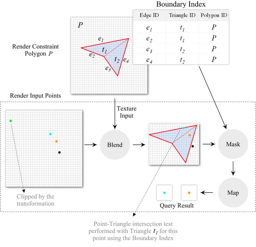
In the case of polygons, the lookup table stores the triangles making up the polygon together with the
unique identifier of the geometry. In addition, we also store a mapping that associates every edge of a polygon
to the triangle incident on it. For example, consider the polygon P in Fig. 4. It consists of 4 boundary edges,
of which e1 and e2 map to the triangle t1 , while the other two edges map to triangle t2 . This mapping is
used during canvas creation to associate each boundary pixel (part of a polygon edge) to the corresponding
triangle. Now, if a geometric primitive intersects with a boundary pixel, to test whether it also intersects with
the corresponding polygon, it is sufficient to simply test if that primitive intersects the triangle indexed by
that boundary pixel. For example, to test whether the cyan point intersects P in Fig. 4, it suffices to simply
test whether this point intersects t1 . Thus, costly point-in-polygon, line-polygon, and polygon-polygon inter-
section tests now become constant time point-triangle, line-triangle, and triangle-triangle tests, respectively.
Brinkhoff et al. [7] had tried out similar index structures where the polygons were partitioned into either
smaller convex polygons, trapezoids, or triangles, which were then stored using the R-tree. As they mention,
this would still require O(n) time in the worst case.
Layer Index. Recall that each geometric object is represented using one canvas. Thus, when working with
data involving millions of objects, the operators need to be executed on millions of canvases. The goal of the
layer index is to reduce the number of canvases created and used, and thus improve the query performance. In
addition, it also improves the GPU occupancy since it allows multiple objects to be processed simultaneously.
It is primarily defined for line and polygon primitives. Given a set of geometric objects (lines or polygons)
that form a canvas, this index partitions the data into a set of layers, such that no two geometric objects in a
given layer intersect. Note that in the worst case, when all objects intersect, each object is in its own layer
which results in the same performance as having no layer index. However, such a scenario is rare in real world
data, thus providing significant query speedup in practice.
5 Spatial Query Engine
The spatial query engine handles planning, optimizing, and executing the queries. In this section, we first
discuss the shader-based implementation of the algebraic operators that are used for different queries–for
their formal definitions, see [10]. We then describe in detail the query evaluation and optimization strategy
followed for the different spatial queries. Finally, we show how the canvas-specific indexes introduced above
can be computed using the GPU operators.
5.1 Implementing the Algebra Operators
Spade implements the following four operators that are summarized in Fig. 3.
Geometric Transform. When a canvas is created, the vertex shader performs the geometric transformation
on the coordinates of the geometries to convert them into screen space. Here, the screen space is defined
based on the query inputs and parameters (e.g., bounds of the selection query polygon), thus clipping (and not
processing) regions that are not touched by the query (e.g., see Fig. 4). It is also used to change the coordinate
system of the underlying data, in particular, from the latitude-longitude based coordinates to the meters-based
EPSG:3857 coordinates for distance and kNN queries.
8Figure 3: Operators implemented in Spade
Mask. The mask operation is implemented in the fragment shader. Fragments are processed in parallel by
the fragment shader, where they are tested against the mask condition. When this condition corresponds
to a polygonal constraint, the corresponding constraint canvas together with the boundary index is used by
the shader to test the mask condition (e.g., see Fig. 4). If the fragment falls on a boundary pixel, then the
appropriate boundary tests are performed. To reduce memory lookup latency, Spade stores the constraint
canvas in the part of the GPU memory that is segregated for textures. Since textures are read-only, hardware
optimizations allow faster data access as compared to traditional global memory.
Multiway Blend. Since spatial data sets are made up of multiple canvases, a single multiway blend oper-
ator becomes beneficial compared to executing multiple blend operations. Hence, Spade implements the
multiway blend operation. For simple blend functions such as additions (used for aggregations), we use the
API-provided alpha blending operation. When the blend function is more complex, or in cases where blend
is combined with other operations, we perform the blending in the fragment shader. The latter scenario is
common when a blend is followed by a mask in a query plan. Since the operations are executed by explicitly
rendering (drawing) the appropriate data, instead of having two (or more) rendering passes, one to perform
blend and one to perform mask, combining the two operations into a single fragment shader helps avoid
unnecessary rendering passes.
9Map (Dissect + Geometric Transform). Since the dissect operation is never used in isolation in any of the
queries, we chose to implement the Map operation as a single operator that performs a dissect followed by a
geometric transform. By definition, the Map operation creates a canvas with a single point for each non-null
fragment of a canvas, where the coordinates of the point are determined by the fragment values. This results
in the creation of numerous canvases, and a naı̈ve implementation becomes expensive.
One approach to overcome this is to implicitly represent each generated canvas within a single output
canvas. Since each of the generated canvases has only one valid point, if we can store each of these points
using unique pixels, then a single output canvas is sufficient. We accomplish this by using the identifiers
associated with the generated canvases to uniquely encode the pixels in the output.
We have two distinct implementations of the Map operation, and the query optimization strategy chooses
the appropriate implementation at runtime based on the query parameters:
1. Given estimate nmax , the maximum possible count of points that are generated by the dissect operation
(described in the following section), a canvas with texture size (resolution) equal to nmax is created, and the
Map operation stores each created point at a unique location within this canvas. This canvas can be thought of
as a list of size nmax having both null and non-null values. When the query is complete, a GPU-based parallel
scan operation [18] is executed (to remove the null elements of the list) and return the result.
2. When the maximum count cannot be estimated, then the Map operation is performed in two steps. The first
step performs a simulated Map operation, counting the number of points created. This count is then used in
the second step to perform the actual Map operation. Note that the second step may require multiple iterations
depending on the count of the points computed in the first step.
5.2 Query Evaluation
Spade closely follows the query plans described in [10,11] for the different spatial queries. Next, we describe
the design choices made in our implementation for the different query types when the data fits into GPU
memory. The following section details how this is extended for off-core processing of large data sets.
Spatial Selection. A spatial selection query identifies all geometric objects from a given query data set
that satisfies a spatial constraint and a select condition. Here the geometric objects can be points, lines,
or polygons, or any combinations of these. Spade currently supports intersection (analogous to the SQL
ST INTERSECTS condition), when the spatial constraint is a polygon.2 In Section 7, we discuss the use
of the containment (SQL ST CONTAINS) condition. The original query plan used for spatial selection [10]
performs a blend followed by a mask operation to generate a set of result canvases. To extract the query result
from the result canvases, we use a modified plan that performs a Map operation following the mask. This
query is implemented in three steps as illustrated in Fig. 4:
1. Create a canvas for the polygonal constraint and store it as a texture. This is done in one rendering pass.
2. Create canvases for the query data set. This is also accomplished in a single rendering pass as follows:
All geometric objects are simultaneously drawn in this rendering pass. Each fragment3 is subjected to the
blend and mask operation, and if the mask condition is satisfied, then the Map operation stores the data
onto an output canvas. This way, the object canvases need not be stored and can be discarded immediately
after the fragments are processed. The query constraint canvas, stored as a texture, is used by the fragment
shader to accomplish the mask operation. Only objects within the query region defined by the bounding
box of the constraint polygon are processed in this step. This is accomplished by defining a transformation
of the input that clips (discards) any object outside this extent, and thus avoiding unnecessary processing.
3. The scan algorithm is used to extract the query result from the output canvas.
2
A rectangular range is also treated as a polygon.
3
Even when multiple objects overlap, overlapping fragments are still processed by shaders. Thus, there is no loss of data even in
such scenarios.
10Figure 4: The steps executed for a selection query. The triangulated polygon is rendered and passed as a
texture during the point rendering phase. As each point is rendered, if it falls outside the bounding box of
the polygon (green point), it is clipped. Points that are not clipped then undergo the blend, mask, and map
operations in the fragment shader. During the mask operation, if the point (cyan point) falls on a boundary
pixel (bold red lines), then a point-triangle intersection test is performed using the boundary index.
Spatial Joins. A spatial join between two spatial data sets, D1 ./ D2 is implemented as a collection of spatial
selections, where the selection constraint is from one of the data sets. The in-memory based implementation of
the join query uses the layer index, introduced earlier. We look at how this is accomplished for the following
two join scenarios:
(1) Polygon ./ Point: Let D1 be the polygon data set and D2 be the point data set. Due to the layer index, each
layer of D1 contains polygons that do not intersect, and thus can be represented in a single canvas texture. Let
there be l layers in the layer index of D1 . The implementation then performs l select operations one for each
layer.
(2) Polygon ./ Polygon: Here, both D1 and D2 are polygonal data sets. Let l1 and l2 be the number of layers
respectively in the two data sets. Without loss of generality, let l1 ≤ l2 . Similar to the previous scenario, l1
selection operations are executed for each of the layers in D1 .
Distance-Based Queries. Distance-based selections and joins differ from spatial selections and joins only in
Step 1: the constraint canvases are created using the geometry shader as defined in Section 4.2.
We support two types of distance-based joins, which are also executed similar to spatial joins:
(1) Given data sets, D1 , D2 , and a distance r, the join returns all pairs of objects (xi , yj ) such that xi ∈ D1 ,
yj ∈ D2 and distance(xi , yj ) ≤ r. The data set with the smaller number of elements is used for creating the
constraint canvases.
(2) Given data sets, D1 , D2 , and a set of distances {r1 , r2 , . . . , rn }, n = |D1 |, the join returns all pairs of
objects (xi , yj ) such that xi ∈ D1 , yj ∈ D2 and distance(xi , yj ) ≤ ri . In this case, constraint canvases are
created on D1 .
11Since the distance parameter of the join query is provided together with the query, unlike polygonal data
sets, it is not possible to have the layer index built beforehand – instead the index is built on the fly during
query execution.
Spatial Aggregations. We support two implementations for the aggregation query. The first performs the
necessary join (or select) followed by the count operation which is accomplished using a geometric trans-
formation followed by a multiway blend. Here, the results from the select (or join) are moved to a unique
location by the geometric transformation, and the blend operation counts the objects in each of these unique
locations to obtain the aggregation result. The second implementation, follows the alternate query plan de-
scribed in [11, Section 5.2]. This plan is customized for aggregations over point data, and uses the multiway
blend, mask, and map operators. This plan first computes partial aggregates of the data using multiway blend,
which are then combined together using the mask and map operations to generate the final result. Query
speedup is obtained in this scenario by avoiding the materialization of the join (or select) results. This is
possible only for points since any given point can be in at most one pixel of the canvas. Note that the latter
implementation is always chosen by the optimizer when working with point data sets.
kNN Queries. Since common real-world kNN queries as well as existing spatial engines support kNN queries
only over point data, we chose to customize the query plan used for kNN queries with respect to point data
as well. Given a spatial data set D, consider a kNN selection query that identifies k points closest to a query
point p. Let B be the bounding box of D. Let rmax be the maximum distance from p to the endpoints of B.
The kNN query is then executed in 3 steps:
1. A circle data set C with c circular constraints is generated, where every circle has center p, and ith circle has
radius ri = rmax
αi
, 0 ≤ i ≤ c and α is a constant > 1. Distance-based canvases are used for this purpose.
A spatial aggregation query is then run on D using C as the constraints. Note that such an approach
might seem inefficient from a traditional CPU algorithmic perspective. However from a computer graphics
perspective, it is designed to harness the GPU as follows. The plan used for aggregation query above
requires just one pass over the polygon constraints irrespective of the number of constraints in the query.
In terms of graphics operations, this amounts to drawing the set of polygons once. GPUs are primarily
designed for this operation4 . Since (i) polygons in this case are simple circles rendered efficiently using
geometry shaders (Section 4.2); and (ii) the number of circles created is logarithmic on the spatial extent
of the input in terms of the canvas resolution, which in practice is at most a few hundreds, the performance
overhead of this step is small.
2. Let ri be the radius of the circle such that aggregation(ci ) ≥ k and aggregation(ci−1 ) < k. A distance-
based selection is now run on D with ri as radius.
3. The query results are then sorted based on the distance to point p, and the k closest points are selected from
the sorted list.
A kNN join is executed similar to the kNN selection query. Let D1 and D2 be the input data sets. Let the
query require identifying the k nearest neighbors of points in D1 . Then, the circle data set containing circles
with varying radii is created for each of the points in D1 in the first step to identify the appropriate radius for
each point in D1 . Then the Type 2 distance join is performed using the computed radii in Step 2. Finally,
similar to the kNN selection query, the query results are sorted based on distance and the required result is
computed.
4
GPUs can render million polygons at rates as high as 60fps
125.3 Out-of-Core Queries
We now discuss how the above query strategies are extended to data that do not fit in GPU memory (and may
or may not fit in CPU memory).
Grid-based index filtering. Spade uses a clustered grid-based indexing structure where each grid cell
corresponds to a block of data that falls into that cell. The block size is tuned based on the system configuration
to ensure that any given grid cell fits into GPU memory (see Section 6.1). The collection of non-empty grid
cells is stored as a set of bounding polygons, i.e., for each cell, instead of storing simply the bounding box,
we store the convex hull over the geometries present in that cell. Thus, the index itself forms a polygonal
data set. When an object spans more than one cell, it is added to the cell that contains its centroid and the
cell’s boundary is expanded. Thus, the cells themselves could intersect unlike in a traditional grid index.
The filtering is then accomplished by executing the appropriate selection/join query on this set of boundary
polygons. Thus, having intersecting cells does not affect the query evaluation strategy.
Due to the use of more detailed polygons instead of bounding rectangles, the index filtering stage of query
execution filters out more data, thus reducing the amount of data used for the refinement stage. Such a strategy
is not used in a traditional setting due to the high processing cost this filtering incurs. However, the overhead
is low in our case since this representation enables the reuse of GPU-based selections and joins to perform
fast index filtering.
Next, we describe the query execution strategy for spatial selections and joins. Other queries are also
executed using a similar strategy. Note that when the data does not fit in CPU memory, the cells of the index
are memory mapped and loaded into the CPU as and when necessary
Spatial Selection. In the index filtering phase of the query, a spatial selection query is first executed on the
bounding polygons (corresponding to the cells) of the clustered grid index to identify all grid cells that satisfy
the selection constraint. For the refinement phase, the GPU in-memory spatial selection query is then executed
on each of these grid cells.
Spatial Joins. Spade incorporates two strategies to perform spatial joins over out-of-core data. The first
makes use of the layer-index based in-memory join described above as follows. Let D1 and D2 be the two
data sets used for the spatial join. The filter phase first performs a Polygon ./ Polygon join over the bounding
polygons of the indexes corresponding to D1 and D2 respectively. This join returns all pairs of grid cells
(gi1 , gj2 ), where gi1 ∈ D1 and gj2 ∈ D2 .
A spatial join is then executed for each pair of grid cells.
The second strategy follows a naı̈ve approach that implements it as a loop of selects. Even though the use
of the layer index decreases the number of canvases involved in the join, since multiple polygons are part of
a single layer (and hence canvas), these layers can cover a large region. Say, data set D1 contains such large-
extent layers, then for each layer, data corresponding to large extents from D2 needs to be transferred to the
GPU. On the other hand, if the individual polygons in D1 cover a relatively smaller region, then depending on
the distribution of the data in D1 and D2 , the total data transferred to the GPU can be significantly lower when
summed over all polygons in D1 . While the layer index-based approach optimizes for the number of rendering
passes, it does not consider the memory transfer. Since the data transfer forms the primary bottleneck in query
execution times, the naı̈ve strategy can therefore perform better in such scenarios.
5.4 Query Optimization Strategies
Spade implements a query optimizer (QO) that performs the following tasks:
Select the appropriate Map operator implementation. The Map operation has two implementations as
described above. It is primarily used to consolidate the results of a query. When the estimate of the query
13result (nmax ) is small enough to fit into the maximum memory allocated for a single canvas, then the 1-pass
Map implementation is used. Otherwise, the 2-pass implementation is used. The result estimation for the
different queries is performed as follows:
1. Selection query: Since each object can either satisfy the query constraint or not, the maximum size of the
output, nmax , is equal to the number of objects.
2. Join query: First, consider Polygon (D1 ) ./ Point (D2 ) joins. Let the number of polygons in ith layer of
the D1 ’s layer index be m, and number of points in D2 be n. The estimate for nmax in this case is n since no
two polygons intersect within a given layer, and a point can intersect only one polygon.
In case of Polygon (D1 ) ./ Polygon (D2 ) joins, let the number of polygons in ith layer of D1 be m, and
number of polygons in D2 be n. Unlike the previous scenario, the estimate of nmax is now n × m (a single
polygon in D1 can intersect multiple polygons in D2 ).
Choose the join implementation. Recall that when a join query is invoked on data sets that do not fit in
memory, Spade supports two join implementations: a naı̈ve approach of executing a set of selections, and
using the layer index. To choose the implementation to be executed, the QO first computes the amount of
data that needs to be transferred to the GPU. For the naı̈ve approach, this is equal to summing the physical
size of the grid cells returned by running the filtering step corresponding to each of the polygons (i.e., a join
between polygons in D1 and bounding polygons of the grid index of D2 ). When the layer index is used, the
required memory is the sum of the sizes of the grid cells returned from the filter step taking into account the
loop order of the join (see next). The join strategy that requires the least memory transfer is then selected and
the corresponding refinement phase is then executed.
Identify the order of join operations. Given a join query, the QO executes this query as a collection of
l selects, where each select constraint corresponds to a layer of the data set D1 (or polygons if the naı̈ve
approach is used). Based on the index filtering using the selection constraint, the appropriate grid cells of
D2 need to be loaded into the GPU for each of the selects. The main idea is for the QO to use this data
transfer overhead to decide on the order of join operations. We chose this simple measure because, as we
show later in the evaluation, the data transfer time forms the primary bottleneck during query execution. In
the current implementation, the QO orders the operations such at least one grid cell or layer (in either D1 or
D2 ) is common between consecutive selects, thus trying to share the memory transfer from one iteration of
the join loop to the next.
5.5 Canvas-Specific Index Creation
Boundary Index. The boundary index has to be created only for polygonal data sets. Let Pb be the set of
lines that make up the boundary of the polygon data. Let Pt be the set of triangles obtained through polygon
triangulation. The required boundary index is then computed by executing a spatial join using Pb and Pt as the
data sets. Note that in this case, each triangle is its own polygon, and hence this data forms a trivial boundary
index for the purpose of this join.
Layer Index. Creating a layer index is accomplished through an iterative process that makes use of the GPU
operators. Consider the ith iteration. When this iteration is executed, i − 1 layers are already computed. Let
Crem = {C1 , C2 , . . . Cn } be set of canvases that have not yet been assigned a layer after i − 1 iterations. Then
the polygons in the ith layer are computed in two passes as follows:
Pass 1: A multiway blend operation is applied on Crem , where the blend function between two objects is
defined such that when two objects overlap, it removes the overlapping regions of the object having a lower
identifier. Let Cmax be the canvas resulting from the above multiway blend operation.
Pass 2: This pass first performs a blend between Crem and Cmax followed by a mask to identify and discard
objects that have been cropped in Pass 1. The objects remaining after the mask operation is used for the
(i + 1)th iteration, and the ones that were discarded are added to the ith layer.
14Spatial # # Physical
Name Type Extent Objects Points Size Description
Taxi Data [25] Points NYC 1.22 B 1.22 B 29 GB Pickup coordinates from taxi trips that happened from 2009-2015
Tweets Points USA 2.28 B 2.28 B 63 GB Geo-locations of tweets gathered using the Twitter API.
Neighborhoods [28] Polygons NYC 195 105.0 K 2.7 MB Neighborhood boundaries of NYC.
Census [27] Polygons NYC 2,165 156.7 K 4.0 MB Census tract boundaries of NYC.
Counties [43] Polygons USA 3,109 5.33 M 134 MB Boundaries of counties within the USA.
Zip Code [44] Polygons USA 32,657 50.53 M 1.3 GB Boundaries of all zip code regions within the USA.
Buildings Polygons World 114 M 764 M 19 GB Building outline polygons from Open Street Map that was used in [31].
Countries [42] Polygons World 250 215.5 K 5.4 MB Boundaries of all countries.
Table 1: Data sets used in our evaluation. A CSV file with only the coordinates was used to compute the size
of the point data sets, while the files in WKT format was used for polygonal data sets (some of these data sets
consists of multi-polygons).
6 Experimental Evaluation
In this section, we first perform an experimental evaluation to assess the efficiency and effectiveness of Spade
using real-world data sets. We then assess the scalability of Spade across query sizes and data distributions
using synthetically generated data. Our main goals are: (1) test the feasibility of using a laptop for spatial
queries over large data sets; and (2) assess the scalability of Spade for different workloads.
6.1 Experimental Setup
Spade Implementation. Spade was implemented using C++ and OpenGL [37], thus allowing it to work
on any GPU and on different operating systems. We chose OpenGL over the more recent Vulkan [20] since
Vulkan drivers are still nascent for many GPUs. Since the OpenGL shaders also works on Vulkan, it is easy
to port Spade to Vulkan in the future.
Data Sets and Queries. Table 1 summarizes the data sets used in the evaluation. To assess the performance
of the system, we chose data sets of varying sizes and spatial extents. In addition, to test SPADE’s ability to
handle large data, we include data sets that are larger than the main memory of commondity machines. Note
that some of these data sets (e.g., taxi, tweets) are larger than those used in a recent evaluation of cluster-based
systems [31].
The workload includes queries with different selectivity (controlled by the regions defined for selection and
join) and reflects queries used in real applications.
While we only use point and polygonal data sets in our experiments, note that the performance of queries
over polygonal data sets can be used as a worst case upper bound for (poly)line data sets—drawing lines and
performing line-intersection tests is cheaper than drawing polygons and performing triangle-intersection tests.
Approaches to Spatial Query Evaluation. Approaches for spatial data analysis can be classified into
three groups based on their target environment: large main-memory servers, map-reduce clusters, and lap-
tops/desktops. We compare Spade against representatives of these groups that were shown to be efficient
in recent experimental studies. Note that the query times across these approaches are incommensurable—it
is not our intent to perform a head-to-head comparison between Spade and these systems. Our goal is to
obtain points of reference to assess the suitability of Spade as an alternative to fill the existing gap for spatial
analytics on commodity hardware as well as better understand the trade-offs involved.
1. Main-memory servers: Common spatial libraries are limited to in-memory processing and thus require
large main-memory servers to handle big data sets. We selected the Google S2 geometry library [17] as
a baseline for the performance on large-memory servers, since a recent study reported that it has the most
consistent performance across query classes [32]. Furthermore, it is optimized for spherical geometry, and is
thus suitable to handle the data sets used in this evaluation.
152. RDBMS: We experimented with PostgreSQL and a commercial database system, and found that these sys-
tems performed significantly slower than the in-memory S2-library. For example, a selection query on the taxi
data that took 5m 21s using the commercial system took only 50s using S2. Similarly, a taxi-neighborhoods
join took close to 3 hours on the commercial system, but only 7m 33s using S2. Moreover, PostgreSQL
performed slower than the commercial system. Therefore, we omit a comparison with these systems.
3. Specialized GPU-based approaches: Several approaches have been proposed that harness the power of
GPUs to support specific queries and/or applications (see Sections 1 and 8). Since these are highly optimized,
they can provide an upper bound for the performance of the query class they support. As a representative of
this class, we selected the open-source GPU-based STIG [12] library, which allows the execution of spatial
selection queries over large point data sets even on laptops. For our evaluation, we used the standalone version
that can be executed independently without MongoDB [38].
4. Cluster-based systems: These systems are specifically designed to handle large data sizes. As a representa-
tive of this class, we selected GeoSpark [48](v1.3.1) for two main reasons: in a recent experimental evaluation
of spatial analytics systems, Pandey et al. [31] found that GeoSpark [48] outperformed the other cluster-based
systems; and it supports a rich set of queries. We tuned GeoSpark for every query that was run (see below).
Since having more nodes in the cluster can increase memory transfer overheads, to be fair, we do not include
the setup (e.g., the time needed to partition and copy data to cluster nodes) and indexing time–we report only
the execution time after the data is already loaded and indexed in the cluster nodes. This setup time is around
half a minute for the smaller polygonal data sets, and it takes 2 and 4 minutes for the larger Taxi and Twitter
data respectively. However, note that there could still be an overhead when the query results from the different
nodes are combined.
Configuration. Spade and STIG were run on a laptop having an Intel Core i7-8750H processor, 16 GB
memory, 512 GB SSD, and a 2 TB external SSD connected via a Thunderbolt 3 interface. The laptop is
equipped with a Nvidia GTX 1070 Max-Q GPU with 8 GB graphics memory. S2 was run on machine with
a 2.40 GHz Xeon E5-2695 processor and 256 GB of RAM. GeoSpark was executed on a cluster with 17
compute nodes, each node having 256 GB of RAM and 4 AMD Opteron(TM) 6276 processors running at
2.3GHz.
Database Setup and Tuning. To evaluate the performance of STIG, indexes were built on the Taxi and
Twitter data sets. The leaf block size was set to 4096 since it gave the best performance compared to other
sizes.
We used the S2PointIndex and S2ShapeIndex for point and polygon data respectively, when using the S2
library.
The performance of GeoSpark depends on multiple parameters: number of partitions (of the SpatialRDD),
spatial partitioning strategy, the spatial index used, as well as the data set order (in case of join queries). We
executed each query multiple times, trying all possible combinations, and used the setting that resulted in the
fastest execution time. Unlike the number of SpatialRDDs, the possibilities for the partitioning strategy, index
type, and data set order are limited. Therefore, to choose the number of partitions, we varied this number
from 4 to 128K to identify the best value for a given query. For all queries, we noticed that the performance
degraded after reaching a peak when the number of RDD partitions became too large. For point data, the
RDD was created using the KDB tree partitioning strategy, while for polygonal data, a Quad tree strategy was
used. An R-tree index was created on each of the partitions for both point and polygon data. Similar to [31],
we followed the guidelines in [9] to tune our cluster.
The grid cell sizes for creating indexes in Spade were selected based on the amount of memory present in
the GPU. Since all the data sets used are GIS-based, we used Open Street Map zoom levels [30] to specify the
grid cell sizes. In particular, we restrict the zoom level such that the maximum size of the data corresponding
to a grid cell is less than 2 GB. Note that this includes not just the coordinates but also the associated metadata
16You can also read